Canton growth in Ecuador and the role of spatial heterogeneity

the role of spatial heterogeneity

Nicola Pontarollo, Rodrigo Mendieta and Diego Ontaneda

Abstract

This paper identifies the determinants of per capita gross value added (GVA) growth in Ecuador during the 2007–2015 period, using a spatial extension of the Mankiw, Romer and Weil (MRW) model. Because as a country Ecuador is characterized by deep territorial socioeconomic imbalances, estimates using classical techniques that measure average or “global” effects would not be as justifiable and would have limited political implications. Accordingly, this study uses a spatial filtering technique, which is a recent evolution of geographically weighted regression (GWR), to account for the spatial heterogeneity of the coefficients of a growth regression that explicitly considers both physical and human capital. The results show that Ecuadorian cantons have a wide range of convergence rates and that the effect of physical and human capital varies across space.

Keywords

Economic growth, economic analysis, regional development, regional economics, econometric models, development indicators, Ecuador.

JEL classification

C21, O47, R11. Authors

Nicola Pontarollo is a Statistics Officer in the Modelling, Indicators and Impact Evaluation Unit of the Competences Directorate at the Joint Research Centre (JRC) of the European Commission1 _{(Ispra, Italy). Email: nicola.pontarollo@ec.europa.eu.}

Rodrigo Mendieta Muñoz is Coordinator of the Research Group on Regional Economics at the Faculty of Economic and Administrative Sciences of the University of Cuenca (Ecuador). Email: rodrigo.mendieta@ucuenca.edu.ec.

Diego Ontaneda Jiménez is a Researcher in the Research Group on Regional Economics at the Faculty of Economic and Administrative Sciences of the University of Cuenca (Ecuador). Email: diego.ontanedaj@ucuenca.edu.ec.

1 _{Neither the European Commission nor any person acting on its behalf is responsible for the use which might be made of the} information contained in this publication. The views expressed herein are of the authors and do not necessarily reflect the position of the European Commission.

I. Introduction

This paper aims to estimate the determinants of economic growth in Ecuador’s cantons, based on a b-convergence model (Baumol, 1986; Barro and Sala-i-Martin, 1992; Mankiw, Romer and Weil, 1992). It examines 214 cantons during the 2007–2015 period.2 _{An alternative spatial technique called “spatial} filtering” (Griffith, 2008) is used to address both spatial dependence and heterogeneity in the impact of independent variables.

Compared to other areas of the world, the literature on subnational economic growth in Latin  America is rather scarce.3 _{In the case of Ecuador, few authors have measured convergence} and the determinants of economic growth, as analysis has been restricted by the absence of reliable economic information at the province and canton levels until 2006. In one of the first studies of the case of Ecuador, Mendieta Muñoz (2015) found conditional convergence between 2007 and 2012 using canton-level data. In the same vein, Ramón-Mendieta, Ochoa-Moreno and Ochoa-Jiménez (2013), concluded, based on province-level data from 1993 to 2011, that there was regional convergence in Ecuador. However, this process is not sufficient to reduce regional disparities. Furthermore, spatial econometric techniques produce results that show that although there is a convergence process, it only involves the cluster of the most developed cantons (Mendieta Muñoz and Pontarollo, 2016). Like the above-mentioned studies, using parametric and non-parametric models Szeles and Mendieta Muñoz (2016) found evidence of absolute and conditional convergence at the canton and province levels for the 2007–2014 period.

This study differs from those described above because it estimates the b-convergence model using an econometric technique —spatial filtering— that takes into account the spatial dependence between canton economies, but which also allows the variables included in the model to have a differentiated effect between cantons, owing to different production structures and contexts. As a result, it is not necessary to assume, as in some previous analyses, that all cantons respond in the same way to variables that affect growth, which is a plausible approach if there are structural differences between cantons.

With respect to spatial dependence, many studies, including those by Fingleton (1999) and Le Gallo and Ertur (2003), have demonstrated that there is spatial correlation in the residuals of traditionally estimated growth models. This leads to an incorrect inference in estimates of significant parameters (spatial error model) or biased and inefficient estimates of parameters (spatial lag model). The spatial filtering technique solves the problem of spatially autocorrelated residuals by taking into account the effects of the spatial interaction between variables. This approach also allows for consideration of the effects of spatial spillovers (Griffith, 2003). In addition, because it is an extension of the geographically weighted regression (GWR) (Fotheringham, Brunsdon and Charlton, 2002) proposed by Griffith (2008), this technique allows for estimation of different local coefficients and not a single coefficient for each variable, as in the ordinary least squares (OLS) method.

2 _{The municipalities of Putumayo, Shushufindi, Cuyabeno, Orellana, La Joya de los Sachas, Sevilla de Oro and Quinsaloma have} been excluded from the analysis because of their atypical gross value added (GVA) values, primarily owing to mineral extraction. 3 _{The countries with the most empirical evidence include Brazil, Colombia and Mexico. Esquivel (1999) and Gomez-Zaldívar,}

Ventosa-Santaulària and Wallace (2012) found evidence of convergence between Mexican regions from 1940 to 1995, and from 1940 to 2009, respectively, while Rodríguez-Pose and Villarreal (2015) focused on the role of socioeconomic conditions according to growth. Cárdenas and Ponton (1995) and Gómez and Santana (2016) focused on Colombian regional convergence and also found evidence of convergence. Royuela and García (2015) confirmed that there is convergence in Colombia in key social variables —although not in the classic economic variable (per capita GDP)— and that spatial autocorrelation reinforces convergence processes. In the case of Brazil, Azzoni (2001) noted that there was regional convergence between 1939 and 1995, but that inequality changed over time. Lastly, De Andrade Lima and Silveira Neto (2016) discovered marked spatial dependence between Brazilian microregions and determined that investments in both physical and human capital are important for the growth of Brazil’s regional economies. This result was confirmed by Resende and others (2016).

Section II describes the spatial dynamics of per capita gross value added (GVA). Section III outlines the empirical model used in the study of growth and details the spatial model employed. Section IV examines the results and section V offers some conclusions.

II. Spatial dynamics of regional growth in Ecuador

The preliminary analysis of spatial dynamics in the case of Ecuador is based on Moran’s I (MI) (Moran, 1950), which is one of the most commonly used means of detecting and measuring spatial dependence (autocorrelation). Moran’s I essentially relates the value of a given variable to its spatial lag, in other words the value assumed by said variable in neighbouring locations. Moran’s I can therefore be defined as:

MI w N x x w x x x x – – – ij j i i i ij j i i i = r r r R R R W W W

/

/

/

/

/

Where N is the number of units on the map (that is to say areas or points); x is the variable of interest; x is the mean of x, and w_ij is an element of spatial weight matrix W_ij, where j represents the set of neighbouring regions to i. Moran’s I generally varies between the maximum and minimum eigenvalue. In a matrix standardized by row, it varies between -1 and 1. A positive coefficient indicates positive spatial autocorrelation, in other words clusters of similar values can be distinguished on the map. A negative coefficient represents negative spatial association, which is to say that dissimilar values are grouped together on the map. A Moran’s I of close to 0 indicates a random spatial pattern.

According to the First Law of Geography of Tobler (1970), which states that “everything is related to everything else, but near things are more related than distant things”, each element i of the W_ij spatial weight matrix is considered to be neighbouring to all other j cantons, but the weight of neighbours is proportional to the inverse of the square distance between the centroids.

This eliminates the need to select ad hoc spatial weight matrices that are based on maximizing the Akaike Information Criterion (AIC) and do not take into account the potential reasons why one definition is more appropriate than another in practice, something that is done by Arbia, Battisti and di Vaio (2010) and Postiglione, Andreano and Benedetti (2017), for example. In addition, it allows for greater interaction between two cantons that have a smaller distance between their centroids than between those that have a larger distance.

The left scale of figure 1 shows the “σ-convergence”, that is to say the dispersion of the (ln) of per capita GVA.4 _{The right scale shows Moran’s I of the same variable for the 2007–2015 period.}5 _The p-value of Moran’s I obtained through 1,000 randomizations is significant for all the years considered. Moran’s I rises very slightly during the period, while σ-convergence shows a much more marked upward trend over time. These patterns indicate that the disparity in per capita GVA between cantons increased during the period of analysis, while polarization remained stable.

4 _{σ-convergence measures the dispersion of territories’ income and shows how, over time, differences between economies tend} to diminish. This means that disparities between territories will tend to diminish over time and therefore approach a single steady state. Following the approach proposed by Barro and Sala-i-Martin (1992), σ-convergence can be measured as the standard deviation of the logarithm of per capita income.

5 _{Per capita GVA was obtained from the data repositories of the Central Bank of Ecuador and from population statistics provided} by the National Institute of Statistics and Censuses (INEC).

Figure 1

Ecuador: σ-convergence and Moran’s I of the log of canton per capita gross value added (GVA), 2007–2015

0 0.05 0.10 0.15 0.20 0.25 0.30 0.20 0.22 0.24 0.26 0.28 0.30 2007 2008 2009 2010 2011 2012 2013 2014 2015 M or an ’s I Var ian ce Variance Moran’s I

Source: Prepared by the authors.

The analysis is complemented by maps of local spatial autocorrelation indexes, used to detect clusters, which is not possible with global spatial association measures. This means that, although global contrasts may indicate a specific spatial autocorrelation, it may not be maintained for the entire sample. Meanwhile, local analysis particularly examines subregions, determining whether such an area represents a hot spot or a cold spot (Celebioglu and Dall’erba, 2010; Cravo and Resende, 2013).

The local Moran statistic (Anselin, 1995) is expressed as:

I_i x x– w x x– N x x i i ij j J j – i 2 i = d r r r R R R W W W

/

/

The Moran statistic fulfils two requirements: (i) it quantifies the degree of significant clustering of similar values around an observation and (ii) it fulfils the need for the sum of the indicator for all observations to be proportional to the global indicator of spatial association. The p-values of the local Moran statistic are based on the Bonferroni correction.

Map 1 shows that while there is a small number of cantons that form clusters that are significant in terms of growth, there are more cantons, and more defined cantons, for per capita GVA in 2007. The significant high-high clusters are located in the areas of Quito and Guayaquil, while the low-low clusters are in the south of the country, in Cañar, and in the central part of the coastal zone.

Map 1

Ecuador: local Moran statistic of the variables included in the model A. Growth in per capita gross value added (GVA), 2007–2015

B. Per capita gross value added (GVA), 2007

Source: Prepared by the authors.

III. The theoretical model, data and

spatial methodology

1. The theoretical model and the data

Our empirical model is based on the concept of conditional b-convergence, which is contrasted using the following cross-sectional econometric model (Mankiw, Romer and Weil, 1992):

ln ln ln ln ln T y y y n g inv h u 1 , , , i i T i i i i i i i it 0 a m 0 r d j c = + + + + + + + U R R R R Z W W W W (3) Where mi=–T−1R1–e−bTW and ai=gi–miSlnAi,0–lnyEi,3X

This means that the mean growth rate of the per capita product of territory i in time period T, to the left of equation (3), is related to its level of per capita product in the initial period (y_i,0). In the constant a_i are the terms g_i(which measures technological progress), A_i,0 (the level of efficiency of each worker) and yE,i3 (steady state). To approximate human capital h, the logarithm of the mean number of years of schooling of people aged 24 and over residing in a given canton was adopted.6 _{The data were} obtained from the 2010 Population and Housing Census. Physical capital, inv, was constructed on the basis of fixed asset information reported by companies in the National Economic Census conducted in Ecuador in 2010. Fixed assets, also known as property, plant and equipment, are tangible assets used by a company in the production or supply of goods or services that are expected to be used for more than one period. δ is the rate of depreciation, n_i is the population growth rate, and, as suggested by Mankiw, Romer and Weil (1992), g+δ has been assumed to be 0.05. Annex A2 shows a mapping of the variables.

The negative and statistically significant coefficient λ_i is used to determine the value of b that approximates the rate of convergence and u_it is the estimation error. The rate of convergence is calculated as β_i = –ln(1 – λ_iT )/T, and the half-life as τ = ln(2)/β_i.7 _{According to Abreu, de Groot and Florax (2005),} standard errors of β_i are obtained as σβ_i =

T 1– i i i v m v b m

R W, where σλi corresponds to the standard errors of λ_i, estimated as indicated by Dawson and Richter (2006) and T is the number of years. Once the errors have been obtained, the t values can be easily determined.

The first studies on convergence (Barro and Sala-i-Martin, 1992) generally analysed this process without adding control variables and assuming that a_i = a and λ_i = λ, that is to say presuming that economies have a homogeneous structure. A negative and statistically significant value of λ indicates that poorer regions grow faster than richer ones, denoting acceptance of the hypothesis of absolute convergence to the same steady state. Thus, as the levels of per capita product of a country’s territory increase, its growth rate should slow, meaning that poor territories grow faster than rich ones and that, in the long term, all of them converge, in per capita terms, to the same rate of income growth and the same level of capital (steady state). Therefore, there is a tendency towards disappearance of the initial economic disparity. However, as Solow (1999, p. 640) states, “there is nothing in growth theory to require that the steady-state configuration be given once and for all” —the steady state will change from time to time, when there are major technological revolutions, demographic changes or changes in the willingness to save and invest.

6 _{This is the variable used as a proxy for human capital in De Andrade Lima and Silveira Neto (2016), De La Fuente (1994),} Benhabib and Spiegel (1994), Barro and Lee (1993) and Kyriacou (1991).

7 _{Half-life refers to the number of years needed to eliminate half the deviation from an initial value of per capita GVA and the value} of the long-run steady state.

Therefore, if there is not the same long-term steady state ln yE,i3, or if structural variables significantly affect growth, then “conditional b-convergence” appears (Sala-i-Martin, 1994; Cuadrado-Roura, Mancha-Navarro and Garrido-Yserte, 2000), which allows for territories not converging towards a common economic equilibrium, but towards individual steady states, determined by specific savings ratios, levels of investment and technology, which are in turn the result of specific economic structures.

As shown in equation (3), to estimate conditional b-convergence a series of additional variables are considered that affect the pattern of growth towards the steady state: physical capital, human capital, and population growth. This approach, which presupposes heterogeneity in the steady states, still assumes homogeneity among convergence rates.

This last point has been criticized by Temple (1998 and 2000), who observes that in a cross-sectional model for different countries, parameter heterogeneity, extreme values and measurement errors are all very frequent. In this regard, Ketteni, Mamuneas and Stengos (2007), and Fotopoulos (2012), for example, find that there is no linearity in processes of economic growth. In terms of regional specificities, however, problems related to spatial dependence must be considered (see, for example, Anselin, 1988; Rey and Montouri, 1999; Arbia, 2006), as well as those related to spatial heterogeneity (Ertur, Le Gallo and LeSage, 2007; Pede, Florax and Lambert, 2014).

In this article, through the use of a model that explores the spatial filtering technique explained in section III.2, the possible presence of heterogeneity is considered, both in the convergence rate, that is to say λ_i = λ, and in the variables that affect growth (Durlauf, Johnson and Temple, 2005). Compared to the article by Cravo and Resende (2013), where the Getis statistic (1995) is used to remove the spatial component from each variable, in this paper the possibility of not only autocorrelation but also non-stationarity is admitted, as explained below.

2. The spatial model

Spatial phenomena are of great importance, especially if consideration is given to socioeconomic factors (Bockstael, 1996; Weinhold, 2002) and to the implications for policymakers (Lacombe, 2004). The presence of spatial patterns that positively or negatively affect economic variables requires rigorous and systematic evaluation of their impact and form. Spatial filters represent a new and interesting research perspective for spatial econometric analysis. This tool can divide geo-referenced variables into two components —spatial and non-spatial— highlighting the spatial autocorrelation component.

The filtration technique proposed by Griffith (2003) uses the technique of decomposition of the matrix into its eigenvectors and eigenvalues, and allows for extraction of the n×n matrix of uncorrelated numerical orthogonal components (Tiefelsdorf and Boots, 1995).

This non-parametric approach aims to manage the presence of spatial autocorrelation by introducing variables —the eigenvectors— that can be used as predictors instead of variables that are not explicitly considered in the model (Fischer and Griffith, 2008). Compared to Getis’s technique (1995), which filters each variable separately by dividing the spatial component from the non-spatial component, this approach offers the advantage that non-negative variables can be used (Griffith, 2010), allowing growth rates, for example, to be included in the analysis.

The model is derived from the matrix form of Moran’s I defined in equation (1):

where W is the matrix of spatial weights, n is the number of cantons, Y is the vector of values and M I –11n

t

=S X is the matrix in which I is the identity matrix of size n×n, 1 is a vector of one dimension n×1 and the exponent t is the transposed matrix. The particularity of the M matrix is that it focuses on the Y vector.

Tiefelsdorf and Boots (1995) showed that each of the n eigenvalues of the expression MWM (4) is an MI value, once multiplied by the term to the left of the expression (4), that is to say _{1 1lW}n .

The eigenfunction linked to the geographical contiguity matrix W can be interpreted as the latent spatial association of a geo-referenced variable (Getis and Griffith, 2002). E1 (the first eigenvector) is the

set of numerical values that has the highest value of MI for the given geographical contiguity matrix. E2 (the second eigenvector) is the group of numerical values that has the greatest value of MI for each

set of numerical values not correlated with E₁. This sequential construction of eigenvectors continues to En a set of numerical values that has the largest MI achievable by any set of numerical values which

is uncorrelated with the preceding n-1 eigenvectors. These n eigenvectors describe the full range of all possible orthogonal and uncorrelated map patterns and may be interpreted as summary map variables that represent the nature (positive or negative) and level (low, moderate, high) of spatial autocorrelation.

The spatial model used in this paper refers to a recent study by Griffith (2008), which proposes a new approach to the GWR model (Fotheringham, Brundson and Charlton, 2002), based on spatial filters through construction of new variables created from the product of the spatial filter and the spatial variables. The spatial filtering approach overcomes the problems of multicollinearity and a lack of degrees of freedom typical of the estimates obtained through the GWR model (Wheeler and Tiefelsdorf, 2005).

The GWR model estimates a “local” regression for each location in space, weighting the observations by distance from the region under study, based on the following expression:

b b = + Y , ,u v 1 Xp p u v, , p P 0 1 f + = R W

/

Where Y is an n×1 vector, and represents the dependent variable, b is the regression coefficient, X_p is an n×1 vector of values of the variable p, e is an n×1 vector containing the random error terms, and (u, v) indicates that the parameters must be estimated for each location whose spatial coordinates are given by the pair of vectors (u, v), implicitly assuming that Y, X and e are geo-referenced.

In his model, referred to here as “GWR-spatial filtering” (GWR-SF), Griffith (2008) proposes the inclusion of an interaction term between each attribute variable and each candidate eigenvector. A normal linear model with spatial filter incorporates a set P of regressors, X_p = (k = 1.2, ..., P), with a k set of selected eigenvectors, E_k = (k = 1.2, ..., K), which represent different spatial models and the following form: = = b +

/

/

/

/

Where • denotes the element-wise matrix multiplication (that is to say Hadamard matrix multiplication) and k_p identifies the eigenvector numbers that describe attribute variable p (k_p being the total number of these vectors). Equation (6) reveals the presence of the interaction terms in question, namely E_kp • X_p. The sum of the first and second terms of equation (6) returns the intercept coefficient expression, while the sum of the third and fourth terms multiplied by X_p, results in the local coefficients of the covariates. Then, by rearranging the results obtained, when all K candidate eigenvectors are considered, yields:

b b = + :

/

/

/

/

Where the regression coefficients represent global values, and the eigenvectors represent local modifications of these global values; the first two terms (that is to say the intercept coefficients and the global attribute variable coefficients) are multiplied by the vector 1, which is also a spatial filter eigenvector. The last two terms are the local variations of the intercept and of the variables themselves. More precisely, the global values are the coefficients needed to construct linear combinations of the eigenvectors, in order to obtain GWR-type coefficients. The estimation of equation (7) needs to be followed by collecting all terms containing a common attribute variable and then factoring it out in order to determine its GWR coefficient, which will be the corresponding sum appearing in equation (6). The GWR coefficients are n×1 vectors. Operationally, the process is as follows:

1. The eigenvectors extracted from contiguity matrix W are computed.

2. All interaction terms Xp • Ek are calculated for the P covariates for the K candidate

eigenvectors (with MI > 0.25).

3. The interaction terms, including the eigenvectors, are selected using step-wise regression, maximizing the value of the Akaike information criterion.

4. The geographically varying intercept term is computed, determined by the first two terms of equation (6).

5. The geographically varying covariate coefficient is computed, determined by the last two terms of equation (6).

IV. Empirical results

This section presents the results of the model described in section III.

Table 1 shows the results of the estimates with ordinary least squares and with spatial filtering of the global coefficients (or means). In order to compare the results of different models, two types of spatial filtering were used: in the first, called SF, individual intercepts are considered, as suggested by Getis and Griffith (2002), selecting the eigenvectors with step-wise regression, to filter spatial autocorrelation in the residuals; the second type is the GWR-spatial filtering approach, which adds to the individual intercepts the eigenvectors associated with each independent variable.

The coefficient of determination R2 _{increases considerably (from 0.35 to 0.72) in the GWR-spatial} filtering, while in the case of spatial filtering with individual intercepts it is 0.53. The Akaike information criterion confirms this result, as does the root mean square error (RMSE), which is used to measure the differences between the values predicted by a model and the values actually observed, which improves markedly in the GWR-SF model. Simultaneously, it is observed that in the second and third models there is no spatial autocorrelation between the residuals, since the Moran test is not statistically significant. Heteroscedasticity persists in the first two models, while the Breusch-Pagan test is not significant in the case of GWR-spatial filtering. The coefficient associated with the logarithm of per capita GVA in 2007 increases marginally in the GWR-spatial filtering model. Education and physical capital are significant in all cases, confirming their role as engines of growth, as has been observed in other Latin American countries. The role of education in Ecuador’s growth confirms the findings of Szeles and Mendieta Muñoz (2016) found with a panel data model for Ecuadorian provinces between 2007 and 2014. The importance of human capital in growth has also been demonstrated in other South American countries, such as Brazil (Cravo, Becker and Gourlay, 2015; Özyurt and Daumal, 2013; De Andrade Lima and Silveira Neto, 2016) and Mexico (Rodríguez-Pose and Villarreal, 2015).

Table 1

Empirical results

Ordinary least squares Spatial filtering GWR spatial filtering

Intercept 0.16838***

(0.06307) (0.06418)0.08086*** -0.04610***(0.05700) Log (per capita GVA 2007) -0.05421***

(0.00616) -0.05696***(0.00555) -0.04803***(0.00525) Population growth 0.006587 (0.01050) -0.01905***(0.01425) -0.03011***(0.01431) Education 0.11562*** (0.01713) (0.01606)0.13553*** (0.01455)0.15128*** Capital 0.00230*** (0.00047) (0.00042)0.00199*** (0.00040)0.00159*** Eigenvector 6 0.11816 (0.03262) Eigenvector 4 -0.12672 (0.03447) Eigenvector 2 0.11593 (0.03327) Eigenvector 28 -0.10626 (0.03354) Eigenvector 29 0.08457 (0.03278) Eigenvector 31 0.07799 (0.03304) Eigenvector 10 0.06993 (0.03350) Eigenvector 15 0.06609 (0.03313) Eigenvector 30 0.06161 (0.03296) Eigenvector 26 0.05558 (0.03281) Convergence coefficient λ 0.07107 0.07603 0. 60610

Residual sum of squares (RSS) 0.03720 0.03250 0.02634

R2 _{(adjusted) 0.354}

(0.342) (0.496)0.529 (0.669)0.724

Akaike information criterion -794.8351 -842.4925 -914.6238

Moran’s I 0.09646*** -0.05453 -0.05572

Breusch-Pagan test 9.729**

(df=4) 23.904**(df=14) (df=35)21.238

Jarque-Bera test 8.0539**

(df=2) 4.0905(df=2) 1.0163(df=2)

Root mean square error (RMSE) 0.03673 0.03136 0.02402

Source: Prepared by the authors.

Note: ***significant at 1%; ** significant at 5%; * significant at 10%; Standard errors in parentheses.

In table 2 the three models are tested, one against another, using the analysis of variance (ANOVA) test. Upon analysing the p-value of the chi-squared test, the conclusion is that both spatial models are significant improvements on the ordinary least squares model. Upon comparing the model estimated using spatial filtering and the GWR-spatial filtering model, the latter can be seen to perform better than the two base models.

Table 2

Analysis of variance (ANOVA) test

Sum of squared deviation Degrees of freedom (df)

Ordinary least squares vs. spatial filters 0.1652*** 31

Ordinary least squares vs. GWR spatial filters 0.0782*** 10

Spatial filters vs. GWR spatial filters 0.0870*** 21

Source: Prepared by the authors.

According to Brunsdon, Fotheringham and Charlton (1998 and 1999), and Fotheringham, Brunsdon and Charlton (2002, p. 229), it is possible to ascertain the non-stationarity of GWR coefficients with two procedures that can be easily extended to GWR-spatial filtering (see table 3).

Table 3

Test for non-stationarity of parameters Variable Standard deviation

bGWR-SF

SE(bOLS) SE(bSF)

Interquartile range bGWR-SF

2×SE(bOLS) 2×SE(bSF)

Intercept 0.3331 0.0631 0.0642 0.2720 0.1261 0.1284

Log (GVA/population) 0.0526 0.0062 0.0055 0.0436 0.0123 0.0111

Population growth 0.0895 0.0105 0.0142 0.0864 0.0210 0.0285

Education 0.0947 0.0171 0.0161 0.0867 0.0342 0.0321

Capital 0.0025 0.0005 0.0004 0.0020 0.0009 0.0008

Source: Prepared by the authors.

The first step is to compare the variance of the GWR coefficients with the standard errors of the coefficients estimated with ordinary least squares. In table 3, all standard deviation values of the GWR-spatial filtering coefficients (second column) exceed the standard errors of the coefficients estimated with stationary models, ordinary least squares and spatial filtering (third and fourth columns). This suggests that there is justification for considering coefficients that vary in space for all coefficients. Secondly, the difference between the lower and upper quartile of the local coefficients (fifth column) must be compared with twice the standard deviations of the respective global estimate (sixth and seventh columns), that is to say ± 1 standard deviation of the mean. The fact that 68% of the values are expected to be within this interval, compared to 50% in the interquartile range, and that the interquartile range of the local coefficients is greater than that of 2 standard errors of the global mean, suggests that the relationship is non-stationary.

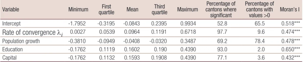
Table 4 shows the local values of the coefficients. To determine whether local coefficients are statistically different from zero, standard errors are calculated taking into account that the latter are derived from the interaction terms (Dawson and Richter, 2006). It is observed that the mean (global) value does not exactly coincide with the value of the coefficient estimated for the variables in table 1, since only local variables that are statistically different from zero are considered in table 4. For all variables there is a marked gap between the first and third quartiles, revealing a high degree of variability. In addition, 98% of cantons show a significant coefficient and about 10% diverge. With respect to the other variables included in the model, population growth rate is significant in 69% of cantons. Surprisingly, education and physical capital are significant in 93% and 77% of cantons, respectively, indicating that there are areas where these variables do not affect growth. This is probably the result of structural heterogeneity, which is reflected in concentration of production sectors in only a few areas; this is usually around the main cities (Mendieta Muñoz and Pontarollo, 2016). The last column represents the Moran’s I of the local coefficients associated with each variable. All the Moran’s Is are positive and significant, reflecting a well-defined spatial pattern, with cantons characterized by similar values located close in space.

Table 4

Local values of significant coefficients

Variable Minimum _quartileFirst Mean _quartileThird Maximum cantons where Percentage of significant Percentage of cantons with values >0 Moran’s I Intercept -1.7952 -0.3195 -0.0843 0.2395 0.9934 52.8 65.5 0.518*** Rate of convergence λ_{i 0.0027} 0.0539 0.0964 0.1191 0.6718 97.7 9.6 0.474*** Population growth -0.3810 -0.0949 -0.0408 -0.0320 0.3487 69.2 78.4 0.478*** Education -0.1762 0.1119 0.1602 0.190 0.4390 93.0 2.0 0.650*** Capital -0.1762 0.1132 0.1593 0.1908 0.4390 77.1 3.6 0.432***

Source: Prepared by the authors.

The foregoing is apparent in table 5, which shows the eigenvectors associated with each variable, together with their geographical scale. These values are mainly used to measure the degree of spatial heterogeneity or spatial homogeneity. In fact, given that, as explained in section III, each eigenvector has an associated Moran’s I, if the prevailing scale of the eigenvectors linked to a variable is the local one, this means that there is marked heterogeneity; that is to say, the phenomenon being studied has an impact on the dependent variable that varies significantly from one territory to another. On the contrary, if the prevailing scale is the global one, the impact of a regressor on the dependent variable does not strongly vary over space. A lack of associated eigenvectors for a variable indicates that the impact of the variable is not differentiated in space. In other words, the impact for each location is the same. In the specific case being analysed, all variables have associated eigenvectors with a predominantly local and regional scale, confirming the existence of well-defined clusters, especially in the mountainous areas, as shown by the local Moran’s I in the maps in annex A3.8

Table 5

Eigenvalues associated with each variable Local scale

(0.50>MI>0.25) (0.75>MI>0.50)Regional scale Global scale(MI>0.75)

Intercept 3 1 1

Log (per capita GVA 2007) 2 3 1

Population growth 3 3 0

Education 3 2 1

Capital 7 1 0

Source: Prepared by the authors.

Map 2 shows the local variation in the coefficient associated with the intercept. The cantons where the structural factors considered by the local value of the intercept have the greatest impact are located in the south of the country and between the coastal and highland regions, in the north of Ecuador. The low-value clusters are in the provinces of Guayas and El Oro.

Map 2

Ecuador: local intercept coefficients

Source: Prepared by the authors.

Note: The dots represent the provincial capitals. 8 _{See annex A1 for the distribution of provinces and areas.}

Map 3 shows the local variation in the convergence rate. The areas with the highest speed of convergence are located in the hot spot of cantons in provinces south of Quito, in the southern part of the country, and on the coast, with the exception of the central-southern area. Lastly, the lowest convergence rates are found in the centre of the mountainous region. In addition, there are certain cantons that diverge (marked with dots), in the province of Cañar and in the north of the country, where clusters of cantons with low convergence rates are also located.

Map 3

Ecuador: rate of convergence λ_i

(Percentages)

Source: Prepared by the authors.

Note: The dots represent the provincial capitals.

Maps 4 and 5 show, respectively, the coefficients for and for physical capital. The first aspect that is apparent is that there are several cantons where coefficients are not significant. With respect to population growth, the cantons are generally located in the central part of the coast, on the border with Peru and on the border with Colombia. Physical capital is not significant in the northern part of the coast, in the Amazon region and in the province of Cañar.

For areas where the population growth rate is statistically significant, the highest coefficients are located in the north-west area. For capital, the impact is greater in the border cantons between the mountains and the coast.

Lastly, map 6 shows how the greatest impact of education is seen in the southern part of the country and in the centre of the mountainous area, where there are statistically significant hot spots of cantons. In addition, clusters with very low impact are observed north of Quito and in Cañar and Azuay.

Map 4

Ecuador: local coefficients of the population growth rate

Source: Prepared by the authors.

Note: The dots represent the provincial capitals.

Map 5

Ecuador: local capital coefficients

Source: Prepared by the authors.

Map 6

Ecuador: local education coefficients

Source: Prepared by the authors.

Note: The dots represent the provincial capitals.

The correlation between the intercept coefficient and the rate of b-convergence is 0.472, indicating that there is a direct but moderate relationship between unobserved structural factors affecting growth and the canton convergence rate (see table 6). In this regard, around half of the cantons with high convergence rates also enjoy certain structural conditions that promote and drive their growth and vice versa. Correlation between the intercept term and the human and physical capital coefficients is negative and very low. In other words, the impact of education and physical capital on canton economic growth is greatest in the cantons where structural conditions are most adverse and vice versa. This shows that the return on investment in human and physical capital is lower in cantons that have achieved a certain degree of development.

Table 6

Correlation between local parameter values

Intercept _λi Population growth Education Capital

Intercept

Rate of convergence _λi 0.472

Population growth 0.175 -0.104

Education -0.258 0.267 -0.099

Capital -0.260 0.257 -0.089 0.813 1

Source: Prepared by the authors.

Furthermore, the correlation between the impacts of human and physical capital shows a positive coefficient of 0.813, meaning that these two factors complement each other. Despite this result, in certain areas of the country —especially the central mountainous area and the Amazon— there is a compensatory effect between physical and human capital: the greater the impact of physical capital, the smaller that of human capital. This may be owing to the economic characteristics of these cantons, which make greater or lesser use of physical and human capital, depending on their production specialization.

V. Conclusions

This paper analyses the process of conditional convergence in Ecuador between 2007 and 2015 through a spatial econometric model that takes into account the structural heterogeneity of the cantons and spatial autocorrelation. Although the model used is an evolution of the GWR approach (Fotheringham, Brunsdon and Charlton, 2002), the GWR-spatial filtering approach does not require coefficients to be non-stationary, but does allow for non-stationarity. This means that in the same regression there may be global and local coefficients, as there would be in a mixed GWR, but with a solution for the problems of multicollinearity and of a lack of degrees of freedom. To assess convergence, per capita GAV is used. As demonstrated in this study, the variance of per capita GAV increases in conjunction with spatial autocorrelation, indicating increasing disparity and economic polarization among cantons.

This analysis differs from previous contributions (Mendieta Muñoz, 2015; Ramón-Mendieta, Ochoa-Moreno and Ochoa-Jiménez, 2013; Mendieta Muñoz and Pontarollo, 2016; Szeles and Mendieta Muñoz, 2016) in that it estimates the conditional b-convergence model using spatial filters, an econometric technique that allows instability of parameters to be taken into account. Therefore, it is not necessary to assume, as in previous studies, that all cantons respond in a similar manner to the factors that determine growth. Instead, the possibility is allowed that the variables in the model have a differentiated effect across space, depending on the particularities of each territory.

In this respect, it is demonstrated that the impact of education is concentrated in the central mountainous area, where there is a clear agglomeration of cities, and near the borders with Peru, which are the fastest-growing areas, where there are more flows of people and goods. Conversely, in the central coastal area, north of Guayaquil, in Cañar, and in the north of the country, education has little or no role with respect to growth. This may be because the cantons that are close to the major cities (Guayaquil, Quito and Cuenca) seem to be sapped by these cities since, according to Mendieta Muñoz and Pontarollo (2016), they absorb resources from nearby areas. The positive impact of physical capital, on the other hand, partially geographically overlaps the effect of human capital.

Lastly, in the context of conditional convergence, highly heterogeneous convergence coefficients indicate that some cantons are close to their own steady state.

The instability in the parameters associated with the spatial dimension shows that in Ecuador there are not only clear inequalities between territories, but also that this situation entails highly asymmetrical effects of factors on convergence. These differences appear to reflect the presence of an element of spatial contagion. This completely changes the connotations of analysis of the factors that affect convergence in the case of Ecuador, meaning that the utmost care must be taken when performing an overall analysis of the country.

It is therefore argued that, in terms of economic policy, emphasis should be placed the need for economic policies to be differentiated to reflect cantons’ different structural characteristics, because regions are not countries and cannot simply replicate national policies at a regional scale (OECD, 2011, p. 19). This relates to the evidence that, as several authors have highlighted (for example, Barca, McCann and Rodríguez-Pose, 2012), in order to draw on the growth potential of a territory there must be a detailed understanding of its socioeconomic structure, in order to adapt local public policy to its particular needs, finding the right combination of actions.

In this regard, the proposed tool, which allows for a deeper understanding of territorial dynamics, can be used to formulate policies that are appropriate to the territorial context and therefore more effective. In the case of Ecuador, which is characterized by marked structural differences, the wrong policies have the potential to harm the country’s balanced development and lead to downward convergence (Szeles and Mendieta Muñoz, 2016), whereby the most developed cantons decline towards the level of the least developed, rather than the other way around.

Bibliography

Abreu, M., H. L. de Groot and R. J. Florax (2005), “A meta-analysis of b-convergence: the legendary 2%”, Journal of Economic Surveys, vol. 19, No. 3, Hoboken, Wiley.

Anselin, L. (1995), “Local indicators of spatial association – LISA”, Geographical Analysis, vol. 27, No. 2, Hoboken, Wiley.

(1988), Spatial Econometrics: Methods and Models, Dordrecht, Kluwer Academic Publishers.

Arbia, G. (2006), Spatial Econometrics: Statistical Foundations and Applications to Regional Convergence, Berlin, Springer.

Arbia, G., M. Battisti and G. di Vaio (2010), “Institutions and geography: empirical test of spatial growth models for European regions”, Economic Modelling, vol. 27, No. 1, Amsterdam, Elsevier.

Azzoni, C. (2001), “Economic growth and regional income inequality in Brazil”, The Annals of Regional Science, vol. 35, No. 1, Berlin, Springer.

Barca, F., P. McCann and A. Rodríguez-Pose (2012), “The case for regional development intervention: place-based versus place-neutral approaches”, Journal of Regional Science, vol. 52, No. 1, Hoboken, Wiley. Barro, R. J. and J. Lee (1993), “International comparisons of educational attainment”, Journal of Monetary

Economics, vol. 32, No. 3, Amsterdam, Elsevier.

Barro, R. J. and X. Sala-i-Martin (1992), “Convergence”, Journal of Political Economy, vol. 100, No. 2, Chicago, The University of Chicago Press.

(1991), “Convergence across states and regions”, Brookings Papers on Economic Activity, vol. 22, No. 1, Washington, D.C., The Brookings Institution.

Baumol, W. J. (1986), “Productivity growth, convergence, and welfare: what the long-run data show”, The American Economic Review, vol. 76, No. 5, Nashville, Tennessee, American Economic Association. Benhabib, J. and M. Spiegel (1994), “The role of human capital in economic development evidence from

aggregate cross-country data”, Journal of Monetary Economics, vol. 34, No. 2, Amsterdam, Elsevier. Bockstael, N. E. (1996), “Modeling economics and ecology: the importance of a spatial perspective”, American

Journal of Agricultural Economics, vol. 78, No. 5, Oxford, Oxford University Press.

Brunsdon C., A. S. Fotheringham and M. Charlton (1999), “Some notes on parametric significance tests for geographically weighted regression”, Journal of Regional Science, vol. 39, No. 3, Hoboken, Wiley. (1998), “Geographically weighted regression-modeling spatial non-stationarity”, The Statistician, vol. 47, No. 3, Hoboken, Wiley.

Canarella, G. and S. Pollard (2006), “Distribution dynamics and convergence in Latin America: a non-parametric analysis”, International Review of Economics, vol. 53, No. 1, Berlin, Springer.

Cárdenas, M. and A. Ponton (1995), “Growth and convergence in Colombia: 1950-1990”, Journal of Development Economics, vol. 47, No. 1, Amsterdam, Elsevier.

Celebioglu, F. and S. Dall’erba (2010), “Spatial disparities across the regions of Turkey: an exploratory spatial data analysis”, The Annals of Regional Science, vol. 45, No. 2, Berlin, Springer.

Cravo, T., B. Becker and A. Gourlay (2015), “Regional growth and SMEs in Brazil: a spatial panel approach”, Regional Studies, vol. 49, No. 12, Abingdon, Taylor & Francis.

Cravo, T. and G. M. Resende (2013), “Economic growth in Brazil: a spatial filtering approach”, The Annals of Regional Science, vol. 50, No. 2, Berlin, Springer.

Cuadrado-Roura, J., T. Mancha-Navarro and R. Garrido-Yserte (2000), “Regional productivity patterns in Europe: an alternative approach”, The Annals of Regional Science, vol. 34, No. 3, Berlin, Springer. Dawson, J. F. and A. W. Richter (2006), “Probing three-way interactions in moderated multiple regression:

development and application of a slope difference test”, Journal of Applied Psychology, vol. 91, No. 4, Washington, D.C., American Psychological Association.

De Andrade Lima, R. and R. Silveira Neto (2016), “Physical and human capital and Brazilian regional growth: a spatial econometric approach for the period 1970-2010”, Regional Studies, vol. 50, No. 10, Abingdon, Taylor & Francis.

De Dominicis, L. (2014), “Inequality and growth in European regions: towards a place-based approach”, Spatial Economic Analysis, vol. 9, No. 2, Abingdon, Taylor & Francis.

De la Fuente, A. (1994), “Crecimiento y convergencia: un panorama selectivo de la evidencia empírica”, Cuadernos Económicos de ICE, No. 58, Madrid, Ministry of Economy, Industry and Competitiveness. Durlauf, S. N., P. A. Johnson and J. Temple (2005), “Growth econometrics”, Handbook of Economic Growth,

Ertur, C., J. Le Gallo and J. P. LeSage (2007), “Local versus global convergence in Europe: a Bayesian spatial econometric approach”, The Review of Regional Studies, vol. 37, No. 1, Southern Regional Science Association.

Esquivel, G. (1999), “Convergencia regional en México, 1940-1995”, Trimestre Económico, vol. 66, No. 264, Mexico City, Fondo de Cultura Económica.

Fingleton, B. (1999), “Estimates of time to economic convergence: an analysis of regions of the European Union”, International Regional Science Review, vol. 22, No. 1, Thousand Oaks, Sage.

Fischer, M. and D. Griffith (2008), “Modeling spatial autocorrelation in spatial interaction data: an application to patent citation data in the European Union”, Journal of Regional Science, vol. 48, No. 5, Hoboken, Wiley. Fotheringham, A. S., C. Brunsdon and M. Charlton (2002), Geographically Weighted Regression: The Analysis

of Spatially Varying Relationships, Chichester, Wiley.

Fotopoulos, G. (2012), “Nonlinearities in regional economic growth and convergence: the role of entrepreneurship in the European union regions”, The Annals of Regional Science, vol. 48, No. 3, Berlin, Springer. Fujita M., P. Krugman and A. J. Venables (1999), The Spatial Economy, Cambridge, MIT Press.

Getis, A. (1995), “Spatial filtering in a regression framework: examples using data on urban crime, regional inequality and government expenditures”, New Directions in Spatial Econometrics, L. Anselin and R. J. Florax (eds.), Berlin, Springer.

Getis, A. and D. Griffith (2002), “Comparative spatial filtering in regression analysis”, Geographical Analysis, vol. 34, No. 2, Hoboken, Wiley.

Gómez, F. and L. Santana (2016), “Convergencia interregional en Colombia 1990-2013: un enfoque sobre la dinámica espacial”, Ensayos sobre Política Económica, vol. 34, No. 80, Amsterdam, Elsevier. Gómez-Zaldívar, M., D. Ventosa-Santaulària and F. Wallace (2012), “Appendix for the PPP hypothesis and

structural breaks: the case of Mexico”, MPRA Paper, No. 41055, Munich, University Library of Munich. Griffith, D. (2010), “Spatial filtering”, Handbook of Applied Spatial Analysis: Software Tools, Methods and

Applications, M. Fischer and A. Getis (eds.), Berlin, Springer.

(2008), “Spatial-filtering-based contribution to a critique of geographically weighted regression (GWR)”, Environment and Planning A: Economy and Space, vol. 40, No. 11, Thousand Oaks, Sage.

(2003), Spatial Autocorrelation and Spatial Filtering: Gaining Understanding through Theory and Scientific Visualization, Berlin, Springer.

Islam, N. (2003), “What have we learnt from the convergence debate?”, Journal of Economic Surveys, vol. 17, No. 3, Hoboken, Wiley.

Ketteni, E., T. P. Mamuneas and T. Stengos (2007), “Nonlinearities in economic growth: a semiparametric approach applied to information technology data”, Journal of Macroeconomics, vol. 29, No. 3, Amsterdam, Elsevier. Krugman, P. (1991), “Increasing returns and economic geography”, Journal of Political Economy, vol. 99,

No. 3, Chicago, The University of Chicago Press.

Kyriacou, G. (1991), “Level and growth effects of human capital: a cross-country study of the convergence hypothesis”, Working Paper, No. 91-26, New York, C.V. Starr Center for Applied Economics, New York University. Lacombe, D. J. (2004), “Does econometric methodology matter? An analysis of public policy using spatial

econometric techniques”, Geographical Analysis, vol. 36, No. 2, Hoboken, Wiley.

Le Gallo, J. and C. Ertur (2003), “Exploratory spatial data analysis of the distribution of regional per capita GDP in Europe, 1980-1995”, Papers in Regional Science, vol. 82, No. 2, Hoboken, Wiley.

LeSage, J. P. and M. Fischer (2008), “Spatial growth regressions: model specification, estimation and interpretation”, Spatial Economic Analysis, vol. 3, No. 3, Abingdon, Taylor & Francis.

Mankiw, N. G. (1995), “The growth of nations”, Brookings Papers on Economic Activity, vol. 1, Washington, D.C., The Brookings Institution.

Mankiw, N. G., D. Romer and D. N. Weil (1992), “A contribution to the empirics of economic growth”, The Quarterly Journal of Economics, vol. 107, No. 2, Oxford, Oxford University Press.

Mendieta Muñoz, R. (2015), “La hipótesis de la convergencia condicional en Ecuador: un análisis a nivel cantonal”, Retos, vol. 5, No. 9, Cuenca, Salesian Polytechnic University.

Mendieta Muñoz, R. and N. Pontarollo (2016), “Cantonal convergence in Ecuador: a spatial econometric perspective”, Journal of Applied Economic Sciences, vol. 39, No. 11, Craiova, ASERS Publishing. Moran, P. A. P. (1950), “Notes on continuous stochastic phenomena”, Biometrika, vol. 37, No. 1-2, Oxford,

Oxford University Press.

Myrdal, G. (1957), Economic Theory and Under-developed Regions, London, Duckworth.

OECD (Organization for Economic Cooperation and Development) (2011), OECD Reviews of Regional Innovation: Regions and Innovation Policy, Paris, OECD Publishing.

Özyurt, S. and M. Daumal (2013), “Trade openness and regional income spillovers in Brazil: a spatial econometric approach”, Papers in Regional Science, vol. 92, No. 1, Hoboken, Wiley.

Pede, V. O., R. J. Florax and D. M. Lambert (2014), “Spatial econometric STAR models: Lagrange multiplier tests, Monte Carlo simulations and an empirical application”, Regional Science and Urban Economics, vol. 49, Amsterdam, Elsevier.

Pina, Á. and M. S. Aubyn (2005), “Public capital, human capital and economic growth: Portugal, 1977-2001”, Focus on Economic Growth and Productivity, L. A. Finley (ed.), New York, Nova Science Publishers, Inc. Postiglione P., M. S. Andreano and R. Benedetti (2017), “Spatial clusters in EU productivity growth”, Growth

and Change, vol. 48, No. 1, Hoboken, Wiley.

Quah, D. (1996), “Regional convergence clusters across Europe”, European Economic Review, vol. 40, No. 3-5, Amsterdam, Elsevier.

Ramón-Mendieta, M., W. Ochoa-Moreno and D. Ochoa-Jiménez (2013), “Growth, clusters, and convergence in Ecuador: 1993-2011”, Regional Problems and Policies in Latin America, J. Cuadrado-Roura and P. Aroca (eds.), Berlin, Springer.

Resende, G. M. and others (2016), “Evaluating multiple spatial dimensions of economic growth in Brazil using spatial panel data models”, The Annals of Regional Science, vol. 56, No. 1, Berlin, Springer.

Rey, S. and B. Montouri (1999), “US regional income convergence: a spatial econometric perspective”, Regional Studies, vol. 33, No. 2, Abingdon, Taylor & Francis.

Rodríguez-Pose, A. and E. Villarreal (2015), “Innovation and regional growth in Mexico: 2000-2010”, Growth and Change, vol. 46, No. 2, Hoboken, Wiley.

Royuela, V. and G. García (2015), “Economic and social convergence in Columbia”, Regional Studies, vol. 49, No. 2, Abingdon, Taylor & Francis .

Sala-i-Martin, X. (1994), “La riqueza de las regiones. Evidencia y teorías sobre crecimiento regional y convergencia”, Moneda y Crédito, No. 198, Madrid, Santander Foundation.

Serra, M. I. and others (2006), “Regional convergence in Latin America”, IMF Working Paper, No. 06/125, Washington, D.C., International Monetary Fund (IMF).

Solow, R. (1999), “Neoclassical growth theory”, Handbook of Macroeconomics, vol. 1, J. B. Taylor and M. Woodford (eds.), Amsterdam, North-Holland.

Szeles, M. and R. Mendieta Muñoz (2016), “Analyzing the regional economic convergence in Ecuador. Insights from parametric and nonparametric models”, Romanian Journal of Economic Forecasting, vol. 19, No. 2, Bucharest, Institute for Economic Forecasting.

Temple, J. (2000), “Growth regressions and what the textbooks don’t tell you”, Bulletin of Economic Research, vol. 52, No. 3, Hoboken, Wiley.

(1998), “Robustness tests of the augmented Solow model”, Journal of Applied Econometrics, vol. 13, No. 4, Hoboken, Wiley.

Tiefelsdorf, M. and B. Boots (1995), “The exact distribution of Moran’s I”, Environment and Planning A: Economy and Space, vol. 27, No. 6, Thousand Oaks, Sage.

Tobler, W. (1970), “A computer movie simulating urban growth in the Detroit region”, Economic Geography, vol. 46, Abingdon, Taylor & Francis.

Weinhold, D. (2002), “The importance of trade and geography in the pattern of spatial dependence of growth rates”, Review of Development Economics, vol. 6, No. 3, Hoboken, Wiley.

Wheeler, D. and M. Tiefelsdorf (2005), “Multicollinearity and correlation among local regression coefficients in geographically weighted regression”, Journal of Geographical Systems, vol. 7, No. 2, Berlin, Springer.

Annex A1

Map A1.1

Ecuador: map of the provinces

Annex A2

Map A2.1

Maps of model variables A. Per capita GVA growth, 2007–2015

C. Population growth, 2007–2015

D. Capital, 2007 Map A1.1 (continued)

E. Mean years of schooling, 2010 (education)

Source: Prepared by the authors.

Note: The dots represent the provincial capitals.

Annex A3

Map A3.1

Local Moran’s I of coefficients A. Local Moran’s I of intercept

C. Local Moran’s I of population coefficient

D. Local Moran’s I of capital coefficient Map A3.1 (continued)

E. Local Moran’s I of education coefficient

Source: Prepared by the authors.

Note: The dots represent the provincial capitals.