<<A>> modelling study of atmospheric cycle of mercury and its exchange processes at environmental interfaces

(1)

(2)

A Modelling Study of Atmospheric Cycle

of Mercury and its Exchange Processes at

Environmental Interfaces

a dissertation presented by

Francesco De Simone to

The Department of Physics

in partial fulfillment of the requirements for the degree of

Doctor of Philosophy in the subject of

Bernardino Telesio Science and Technology Doctorate School University of Calabria

Rende, Italy November 2015

(3)

(4)

Thesis advisor: V. Carbone, N. Pirrone, I. M. Hedgecock Francesco De Simone

A Modelling Study of Atmospheric Cycle of Mercury and its

Exchange Processes at Environmental Interfaces

Abstract

Since ancient times human activities have significantly altered the natural global Mercury (Hg) cycle through emissions to the environment. Hg is a global pollu-tant since its predominant atmospheric form, elemental Hg, reacts relatively slowly with the more abundant atmospheric oxidants and is therefore transported long distances from its emission source. Once oxidised however Hg is readily deposited, an can then be converted to the toxic monomethylmercury (MeHg) in soils and natural waters. MeHg is able to bioaccumulate and biomagnify, up to levels at which it is harmful to human health. Mercury pollution is therefore a threat to ecosystem health on a global scale, and is now being addressed by an international agreement, the Minamata Convention. Comprehensive knowledge of the details of the atmospheric Hg cycle is still lacking, and in particular there is some un-certainty regarding the atmospherically relevant reduction-oxidation reactions of mercury and its compounds. The exchange of Hg and its compounds between the atmosphere and the oceans also plays an important role in the cycling of mercury in the environment: understanding and quantifying mercury deposition patterns and fluxes is critically important for the assessment of the present, and future, en-vironmental impact of mercury contamination. ECHMERIT is a global on-line chemical transport model, based on the ECHAM5 global circulation model, with a highly customisable chemistry mechanism designed to facilitate the

(5)

investiga-Thesis advisor: V. Carbone, N. Pirrone, I. M. Hedgecock Francesco De Simone

tion of both aqueous and gas phase atmospheric mercury chemistry. An improved version of the model which includes a new set of emissions routines, both on-line and off-line, has been developed and used for this thesis to investigate and assess a number of the uncertainties related to the Hg atmospheric cycle. Outputs of multi-year model simulations have been used to validate the model and to esti-mate emissions from oceans. Various redox mechanisms have been included to assess how chemical reactions influence the models ability to reproduce measured Hg concentrations and deposition flux patterns. To characterize the Hg emissions which result from Biomass Burning , three recent biomass burning inventories (FINNv1.0, GFEDv3.1 and GFASv1.0) were included in the model and used to investigate the annual variation of Hg. The differences in the geographical distri-bution and magnitude of the resulting Hg deposition fluxes, hence the uncertainty associated with this Hg source, were quantified. The roles of the Hg/CO enhance-ment ratio, the emission plume injection height, the Hg0_(g)oxidation mechanism and lifetime, and the inventory chosen, as well as their uncertainty were consid-ered. The greatest uncertainties in the total deposition of Hg due to fires were found to be associated with the Hg/CO enhancement ratio and the emission in-ventory employed. Deposition flux distributions proved to be more sensitive to the emission inventory and the oxidation mechanism chosen, than all the other model parameters. Over 75% of Hg emitted from biomass burning is deposited to the world’s oceans, with the highest fluxes predicted in the North Atlantic and the highest total deposition in the North Pacific. The net effect of biomass burning is to liberate Hg from lower latitudes and disperse it towards higher latitudes where it

(6)

is eventually deposited. Finally, the model was used to evaluate the fate of the Hg released into the atmosphere by human activities. Anthropogenic emissions are estimated to amount to roughly 2000Mg/y (1000-4000 Mg/y). Hg speciation (el-emental, oxidised or associated with particulate matter) is subject to many uncer-tainties: the extremely variable lifetimes among Hg species, as well as the Hg emis-sion heights, in combination with the complex physical and chemical mechanisms that drive its final fall-out lead to considerable uncertainties. To address this spe-cific issue three anthropogenic Hg emission inventories, namely AMAP-UNEP, EDGAR and Streets, were included in the Model. Different model parametrisa-tions were adopted to trace the fate of Hg to its final receptors and to thoroughly test the model performance against the measurements. Primary anthropogenic Hg contributes up to 40% of the present day Hg deposition. The oxidation mech-anism has a significant impact on the geographical distribution of the deposition of Hg emitted from human activities globally, : 63% is deposited to the world’s oceans. The results presented in this thesis provide a new and unique picture of the global cycle of mercury, evaluating and assessing the uncertainties related to many aspects with an on-line Global Circulation Model developed specifically to investigate the global atmospheric Hg cycle.

(7)

Sin dall’antichità, le attività umane hanno alterato il naturale ciclo del Mercurio attraverso il suo rilascio incontrollato nell’ambiente. Il Mercurio è un inquinante a diffusione globale in quanto la sua forma atmosferica predominante, detta Mer-curio elementare, interagisce molto lentamente con i principali ossidanti presenti in atmosfera, e può essere quindi trasportato molto lontano dalle sorgenti di emis-sione. Comunque, il Mercurio, in seguito alla sua ossidazione, viene rapidamente depositato e può essere convertito in monometilmercurio (MeHg) sia nel suolo che nelle acque. Il monometilmercurio è in grado di accumularsi nei tessuti bi-ologici, biomagnificandosi all’interno della catena alimentare fino a raggiungere livelli pericolosi per la salute umana. L’inquinamento da Mercurio è quindi una minaccia alla salute degli ecosistemi su scala planetaria, e, per tal motivo, è stato di recente oggeto di un accordo internazionale, noto come Convenzione di Mina-mata. La conoscenza dei dettagli riguardanti le fasi del ciclo del mercurio in atmos-fera è molto lontana dall’essere completa. In particolare le incertezze riguardano le reazioni di ossido-riduzione a cui vannno incontro in atmosfera il mercurio e i suoi composti. Lo scambio del mercurio all’interfaccia atmofera-oceano è un al-tro elemento chiave nel ciclo del mercurio: la comprensione e la quantificazione di questi processi di scambio sono critici per una corretta valutazione dell’impatto sull’ambiente della contaminazione da mercurio.

ECHMERIT è un modello globale numerico di tipo on-line per lo studio del trasporto e della chimica, basato sul modello di circolazione globale ECHAM5. Dispone di un meccanismo chimico altamente personalizzabile e progettato per lo studio della chimica del mercurio in atmosfera sia nella fase gas che in quella

(8)

acquosa.

Per questo lavoro di tesi è stata sviluppata una versione migliorata del modello, che include un nuovo set di routine per la gestione delle emissioni, sia calcolate dinamicamente nel modello, sia importate off-line da campi esterni. Il modello così modificato è stato utilizzato per lo studio e per la valutazione delle incertezze relative alle diverse fasi del ciclo atmosferico del mercurio. I risultati ottenuti da simulazioni di diversi anni sono stati usati preliminarmente per validare il mod-ello e per stimare le emissioni di mercurio dagli oceani. E’ stato inoltre valutato l’impatto di diversi meccanismi chimici sulla capacità del modello di riprodurre i livelli di concentrazione e di deposizione di mercurio misurati. Per caratteriz-zare le emissioni di mercurio dalla cosiddetta combustione di biomassa (Biomass Burning), sono stati inclusi nel modello tre inventari recenti per questo tipo di emissioni (FINNv1.0, GFEDv3.1 e GFASv1.0). Si è quindi studiata la variazione annuale delle emissioni di mercurio dai fuochi, oltre alla distrubuzione geografica delle deposizioni risultanti. E’ stato inoltre valutato il ruolo dei rapporti di arricchi-mento Hg/Co, l’altezza del plume delle emissioni, i meccanismi di ossidazione e i tempi di residenza in atmosfera del mercurio elementale, l’inventario utilizzato e caratterizzata l’incertezza di ciascuno di questi elementi. La più grossa fonte di incertezza sull’entità delle deposizioni di mercurio emesso dai fuochi è stata trovata essere associata al raporto di arricchimento Hg/CO e all’inventario uti-lizzato. La distribuzione dei flussi di deposizione è stata provata essere più sensi-bile all’inventario e al meccanismo di ossido-riduzione adottato, che a tutte le altre parametrizzazioni adottate. Più del 75% del mercurio rilasciato dai fuochi viene

(9)

depositato sugli oceani. Il più alto flusso è stato simulato nell’Atlantico del nord, mentre la deposizione totale più alta nel Nord Pacifico. L’effeto netto della com-bustione di biomassa è risultato quello di liberare mercurio dalle basse latitudini e di disperderlo nelle alte, dove eventualmente si deposita. Infine, il modello è stato utilizzato per valutare il destino del mercurio rilasciato in atmosfera dalle attiv-ità antropogeniche. Le emissioni antropogeniche si stima ammontino grossolana-mente a circa 2000 Mg/a (con un margine che va da 1000 a 4000 Mg/a). An-che la speciazione delle emissioni, ovvero la forma in cui viene emesso (mercurio elementare, ossidato o associato a particolato) è incerta: la grande differenza nei tempi di residenza in atmosfera delle diverse specie di mercurio, così come l’altezza del rilascio delle emissioni in combinazione con i complessi e misconosciuti pro-cessi fisici e di trasformazione che guidano laricaduta finale del mercurio genera un’incertezza ancora maggiore riguardo i recettori finali. Per valutare specificata-mente queste problematiche, son stati inclusi nel modello tre inventari per le emis-sioni antropogeniche di mercurio, AMAP-UNEP, EDGAR and Street. Sono state quindi adottate diverse parametrizzazioni per seguire la destinazione finale del mer-curio e per valutare le performance del modello in termni di confronto con le mis-ure disponibili. Le emissioni antropogeniche primarie di mercurio contribuiscono fino al 40% delle deposizioni locali and the 63% of mercury emitted is deposited to oceans. I risultati presentati in questa tesi forniscono una vista unica sul ciclo del mercurio in atmosfera, in quanto permettono di valutare le incertezze di molti aspetti con un modello di Circolazione generale globale di tipo on-line sviluppato appositamente per lo studio del ciclo atmosferico del Mercurio.

(10)

Author List

(13)

Listing of figures

1.1.1 Ice core record of Hg deposition Upper Fremont Glacier. Image from [122]. . . 3 1.1.2 Global Hg budget illustrating the natural and anthropogenic

emis-sions sources and the cycle between the main environmental com-partments. Image from UNEP [121]. . . 5 1.1.3 Global anthropogenic Hg emissions in 2010. Image from UNEP

[121]. . . 6 1.1.4 Long-range Hg transport. Image from [121]. . . 7 1.1.5 Global cases of Hg poisoning incidents. Image from [121]. . . . 9 2.4.1 Geographical distribution of Total Gaseous mercury (TGM)

sur-face concentration (ng/m3_{) as resulted by using different full}

chem-istry mechanism: a) Base, b) Base2, c) Base4, d) Base3. Model values are annually averaged for the simulation period (2008-2009).

22

2.4.2 Hemispherical gradient of total gaseous mercury (TGM) as re-sulted by using different full chemistry mechanism. Model data are averaged longitudinally for the 2008-2009 simulated period. . 23

(14)

2.4.3 Averaged latitudinal distribution of air concentrations of Hg0_as

simulated by base Model. Red shadowed area represents the 1st to 99th _{percentile range of the longitudinal variation. Annually} averaged measurements are also reported: circles indicates mea-surements collected during the same years of the simulation pe-riod. Observations include those used by [119] plus additional sites in Europe belonging to EMEP programme . . . 25 2.4.4 Spatial distribution of annually averaged air concentrations of Hg0

and HgII_{. The background model simulated data and the}

mea-surements for Hg0_{are the same of Figure 2.4.3. Hg}II_observations

include those used by [119] plus additional sites in Europe be-longing to EMEP programme . . . 26 2.4.5 Mean seasonal variations of TGM at northern mid-latitudes.

Ob-servations are annual means averaged over 6 EMEP sites. Shad-owed area indicates the standard deviation for observations. . . 27 2.5.1 (a) Global distribution of Hg0fluxes from oceans surface. Fluxes

are annual mean values from the model simulation period. (b) Latitudinal distribution of the oceanic Hg0_{Flux, in different}

sea-sons, and the annual mean. . . 29 2.6.1 Global distribution of wet deposition fluxes during the

simula-tion period . . . 31 2.6.2 Annual Hg wet deposition fluxes over North America during

2008-2009 as simulated by base model. Overlaid circles show wet de-position observed during the same years by Mercury Dede-position Network (MDN) . . . 32 2.6.3 Seasonal Hg wet deposition fluxes over North America averaged

over 2008-2009 period, as simulated by base model (background) and observed by MDN sites (Circles). . . 33 2.6.4 Annual Hg wet deposition fluxes over Europe during 2008-2009

as simulated by base model. Overlaid circles show wet deposition observed during the same years by EMEP sites. . . 35

(15)

2.6.5 The total annual global Hg budget as derived from the base model. Emission and deposition rates are given in Mg y−1. Inventories are in Mg. . . 36 3.2.1 Validation of the Base Model. Note that the deposition scatter

plot has a log scale (both for x and y) to better visualize the outliers. 46 3.2.2 Validation of Br-Based Model using the GFED inventory.

Perfor-mance is compared to the GFED Base simulation. Note that the deposition scatter plot has a log scale (both for x and y) to better visualize the outliers. . . 47 3.2.3 Validation of the 12 month fixed lifetime using the GFED

inven-tory. Performance is compared to the GFED Base simulation. Note that the deposition scatter plot has a log scale (both for x and y) to better visualize the outliers. . . 48 3.2.4 Annual trends and averaged latitudinal profiles of mercury

emis-sions ((a) and (c)) and deposition ((b) and (d)). Figure (b) ex-cludes 2006 due to low re-emissions, see section 3.2.2 . . . 49 3.2.5 Geographical (left), seasonal (center, DJF - December January

February, MAM - March April May etc.) and regional (right) dis-tribution of mercury emissions. Annual averages over the 2006– 2010 period. The regions are, following the nomenclature used in van der Werf et al. [125], (Boreal North America (BONA), Temperate North America (TENA), Central America (CEAM), Northern Hemisphere South America (NHSA), Southern Hemi-sphere South America (SHSA), Europe (EURO), Middle East (MIDE), Northern Hemisphere Africa (NHAF), Southern Hemi-sphere Africa (SHAF), Boreal Asia (BOAS), Central Asia (CEAS), Southeast Asia (SEAS), Equatorial Asia (EQAS) and Australia (AUST) . . . 51

(16)

3.2.6 Geographical distribution of the total mercury deposition (wet + dry) that result from BB. Annual averages over the 2007–2010 period. . . 52 3.2.7 Latitudinal profile of annual Hg net deposition flux (Deposition

- Emission), averaged over the period 2007–2010. . . 54 3.2.8 Agreement map of Hg deposition fields obtained from GFAS,

GFED and FINN for the five year simulation. The map shows the areas where deposition is > μ+σ. Primary colors (red, blue and yellow) represent non-agreement between inventories, green, pur-ple and brown indicate agreement between two of the inventories and gray indicates agreement between all three. The numbers re-fer to the number of cells in common between the simulations using the different inventories (The whole globe is represented by 8192 cells) . . . 56 3.2.9 Agreement maps of Hg deposition for GFED, GFAS and FINN,

for the single year simulations. The maps show the areas where deposition is greater than μ+σ. Primary colors (red, blue and yel-low) represent non-agreement between inventories, green, pur-ple and brown indicate agreement between two of the invento-ries, and gray indicates agreement between all three. The num-bers refer to the number of cells in common between the simu-lations using the different inventories (The whole globe is repre-sented by 8192 cells) . . . 58

(17)

3.2.10Agreement maps for Hg deposition exceeding μ+σ for simula-tions using the Base (O3+OH) and the Br-based oxidation

mech-anisms, and fixed Hg0 _{lifetimes of 6 and 12 months. The map}

shows the areas where deposition is > μ+σ. Primary colors (red, blue and yellow) represent non-agreement between inventories, green, purple and brown indicate agreement between two of the inventories and gray indicates agreement between all three. The numbers refer to the number of cells in common between the simulations using the different inventories (The whole globe is represented by 8192 cells) . . . 62 3.2.11Geographical distribution of the probability density function of

the total Hg deposition obtained from an inspected ensemble of simulations for the year 2010. Total deposition is illustrated in terms of the average (μ) and standard deviation σ of the ensemble. 65 4.1.1 Geographical distribution of annual mercury emissions and the

latitudinal vertical profile of the increase in atmospheric Hg con-centration resulting from anthropogenic emissions as estimated by STREETS, EDGAR and AMAP inventories. . . 72 4.2.1 Agreement map of Total Hg emissions for the AMAP2010, EDGAR

and STREETS inventories. The map shows the areas where the emissions are > μ+σ. Primary colors (red, blue and yellow) rep-resent non-agreement between inventories, green, purple and brown indicate agreement between two of the inventories and gray indi-cates agreement between all three. The numbers refer to the num-ber of model cells in common between the different inventories, the whole globe is represented by 8192 cells. . . 76

(18)

4.2.2 Latitudinal profiles of mercury emissions (a) and normalised to-tal deposition that result from model runs adopting O₃+ OH (b) and Bromine (c) driven oxidation mechanism for the different inventories. Panels (a) and (b) reports deposition obtained by including all emission sources (plus re-emissions) and only an-thropogenic emissions. Deposition profiles are not in scale. . . . 78 4.2.3 The latitudinal profile of the simulated wet deposition flux using

the three inventories and the both atmospheric oxidation mech-anisms . . . 80 4.2.4 Geographical distribution of the total mercury deposition (wet

+ dry) that result from model runs including all sources, for the three inventories and the two oxidation mechanisms. . . 81 4.2.5 Geographical distribution of the total mercury deposition (wet

+ dry) that result from model runs including only anthropogenic emission sources for the three inventories and the two oxidation mechanisms. . . 83 4.2.6 Agreement maps of Hg deposition fields obtained from runs

con-sidering STREETS, EDGAR and AMAP inventories and includ-ing all emission sources plus re-emissions (a and c) and only an-thropogenic emissions (b and d). Maps are computed for both oxidation mechanism adopted: Bromine (c and d) and OH+_O

3

(a and b). The maps show the areas where deposition is > μ+σ. 84 4.2.7 Geographical distribution of the total Hg deposition from

anthro-pogenic emissions only obtained from an inspected ensemble of simulations for the year 2010 (a) in terms of the average (μ) and standard deviation σ of the ensemble. In (b) such distribution is compared with the ensemble of the same simulations including all other emission source to have a Geographical distribution of the impact. . . 86 A.5.1 Map of the distribution ERfine . . . 96

(19)

(20)

(21)

I’m investigating things that begin with the letter M. The Mad Hatter, from Alice in Wonderland (2010)

1

Introduction

The Earth’s atmosphere is a mixture a of a number of gases, each with its own pro-prieties, that encircle our planet. It consists of about 78 percent nitrogen and about 21 percent oxygen. The remaining one-percent contains all the other gases in-cluding carbon monoxide, carbon dioxide, ozone, methane, ammonia along with a wide variety of trace chemical compounds. Air pollution occurs when one or more of these elements or compounds reach harmful concentrations. That is, concen-trations which could be harmful to the health or comfort of humans and animals or which could cause damage to plants and materials. The substances that cause air pollution are collectively called pollutants and are emitted at any moment by such natural occurrences as volcanic eruptions, forest fires, decaying vegetation as well as by human activities. Air pollution is nothing new. In medieval Eng-land, where the burning of coal was the primary method people had for heating, the black smoke from chimneys caused many problems. This pushed the King, in

(22)

1306, to regulate the use of coal. Although these efforts failed to solve the prob-lem, historically, they represent the first set of air pollution ordinances in attempt to clean the air [124]. While the problem of air pollution has existed for centuries, the present day industrial boom and population explosion have made it critical and only during the past few decades have we begun to understand that air is a resource that has to be managed for health and environmental quality.

1.1 Hg Air pollution

Mercury (Hg) and particularly methylmercury compounds (MeHg) are extremely toxic and represents a threat to the environment and ecosystems, and also for hu-man health. Mercury is a natural element and is found throughout the world. The natural sources of Hg are many and background environmental levels have been present since long before the human race appeared. Hg is contained in many min-erals, including cinnabar (HgS), an ore mined to produce Hg, however much of the present day demand for Hg is met by recovery Hg from industrial sources. Hg is also present as an impurity in many other minerals, such as gold and non-ferrous metal ores, and also fossil fuels, particularly coal. Human activities, mining and the burning of coal have increased the release of Hg into the environment, raising its burden in all environmnetal compartments: atmosphere, soils, fresh waters, and oceans. The majority of these human Hg emissions have occurred since the in-dustrial revolution in 1800 and are continuing with fossil-fuel-based energy gen-eration powering industrial and economic growth in South and South-East Asia [79,110,121] (See Figure 1.1.1).

Even now, Hg is commonplace in daily life. Electrical and electronic devices, switches (including thermostats) and relays, measuring and control equipment, energy-efficient fluorescent light bulbs, batteries, mascara, skin-lightening creams and other cosmetics which contain Hg compounds, dental fillings and a host of other consumables are used across the globe. Food products obtained from fish, terrestrial mammals and other products such as rice can also contain Hg. It is still

(23)

Figure 1.1.1: Ice core record of Hg deposition Upper Fremont Glacier. Image

(24)

widely used in health care equipment, where it is used in measurement equipment such as in sphygmomanometers (to measure blood pressure) and thermometers, although their use is declining.

1.1.1 Hg Emissions and Remedies

Hg is emitted in the atmosphere from a variety of sources, as illustrated in Figure 1.1.2. Estimates of natural emissions are in the range of 4000 to 7000 Mg yr−1 [121]. Natural sources include crustal degassing, volcanoes, the re-emission of previously deposited Hg from soils and aquatic surfaces, weathering processes of the Earth’s crust and forest fires [78]. Contributions from natural sources and processes vary geographically and temporally depending on a number of factors including meteorological conditions, the presence of volcanic or geothermal ac-tivity, the presence of Hg and also the occurrence of forest fires [37,78]. The two major source categories include those related to the geological presence of Hg in various minerals and evasion of Hg from aquatic and terrestrial ecosystems. This latter is related to the historical atmospheric deposition of Hg to these ecosystems, that originally was emitted by both natural and anthropogenic sources. Therefore it is not simple to distinguish between the emission of ’legacy’ Hg and Hg emitted form natural sources.

Global emissions of Hg to the atmosphere in 2010 from human activities were estimated at 1,960 tonnes and appear to have been relatively stable from 1990 to 2010 [122]. Globally more than half of the Hg from anthropogenic sources is emit-ted as GEM, or Hg0, while only 10% of emissions occur as PBM, or Hgp. The rest of the Hg is emitted as GOM, or HgII_[₁₂₂_]

The largest anthropogenic sources are associated with artisanal and small-scale gold mining (ASGM) and coal burning, and together contribute about 61% of an-nual anthropogenic emissions to the atmosphere. Other major contributors in-clude ferrous and non-ferrous metal production and cement production, together responsible for 27% (See Figure 1.1.3).

(25)

Figure 1.1.2: Global Hg budget illustrating the natural and anthropogenic

emissions sources and the cycle between the main environmental

(26)

Figure 1.1.3: Global anthropogenic Hg emissions in 2010. Image from UNEP

[121].

Hg residues from mining and industrial processing, as well as Hg in waste, have resulted in a large number of contaminated sites all over the world. Most Hg con-taminated sites are concentrated in the industrial areas of North America, Europe and Asia; and in sub-Saharan Africa and South America.

Air pollution control technologies in industrial facilities remove Hg that would otherwise be emitted to the air. Although there is little information about the ul-timate fate of the Hg captured in this way, it is likely that these control technolo-gies will reduce the amount of Hg that is transported globally by the atmosphere. For many health care applications and for pharmaceuticals there are safe and cost-effective replacements for Hg, and the goal to reduce demand for Hg-containing fever thermometers and blood pressure devices by at least 70% by 2017 has been set[121].

However while the atmosphere responds relatively quickly to changes in Hg emissions, the large reservoirs of Hg in soils and oceans mean that there will be

(27)

Figure 1.1.4: Long-range Hg transport. Image from [121].

a long time lag (on the order of years to decades [11]) before reductions in Hg inputs are reflected in depleted concentrations in these media and in the wildlife taking up Hg from them. Therefore it is necessary to act now to reduce ecosystem exposure to Hg in next decades [121].

1.1.2 Effects on Human Health

Differently from other pollutants that are restricted in their range and in the size and number of the populations they affect, wherever Hg is mined, used or dis-carded, it is liable to finish up thousands of kilometres away because of its lifetime in the atmosphere and oceans[11,121] (See Figure 1.1.4).

(28)

predator fish such as swordfish and shark that may be consumed by humans. There can also be serious impacts on ecosystems, including reproductive effects on birds and predatory mammals. High exposure to Hg is a serious risk to human health and to the environment [121]. Atmospheric emissions of Hg are highly mobile globally, while aquatic releases of Hg are more localised. Hg in water becomes more biologically hazardous when it is methylated and enters the food chain, al-though some is eventually reduced to Hg0and evades to the atmosphere. Equally in soils and sediments, Hg can be methylated, largely through metabolism by bac-teria or other microbes, and can enter the food chain and ultimately be of concern to human health [121]. Hg can seriously harm human health, and is a particu-lar threat to the development of foetuses and young children. It affects humans in several ways. At very high air concentrations Hg vapour is rapidly absorbed into the blood stream when inhaled. It damages the central nervous system, thy-roid, kidneys, lungs, immune system, eyes, gums and skin. Neurological and be-havioural disorders may be signs of Hg contamination, with symptoms including tremors, insomnia, memory loss, neuromuscular effects, headaches, and cognitive and motor dysfunction. In the young it can cause neurological damage resulting in symptoms such as mental retardation, seizures, vision and hearing loss, delayed development, language disorders and memory loss [121].

People may be at risk of inhaling Hg vapour from their work (in industry or ASGM), or in spills, and may be at risk through extended direct contact of Hg with the skin. The most common form of direct exposure for humans, however, is through consuming fish and sea food contaminated with methylmercury. Once ingested, 95 per cent of the chemical is absorbed in the body [121].

A continuous release of the toxic methylmercury in the industrial waste water from the Chisso Corporation’s chemical factory from 1932 to 1968 was the cause of the greatest local Hg poisoning event in the history. The so called Minamata disease was first discovered in Minamata city in Kumamoto prefecture, Japan, in 1956. Symptoms included numbness in the hands and feet, general muscle weak-ness, narrowing of the field of vision, and damage to hearing and speech (EINAP). In extreme cases, insanity, paralysis, coma and death have been known to ensue

(29)

Figure 1.1.5: Global cases of Hg poisoning incidents. Image from [121].

rapidly. As of March 2001, 2,265 victims had been officially recognised as having Minamata disease (1,784 of whom had died) ¹. Unfortunately, this is only one ex-ample of the poisoning events which have occurred. Figure 1.1.5 summarizes the global cases of Hg poisoning incidents [121].

Hg pollution is therefore a threat to ecosystem health on a global scale, and is now being addressed as such following the negotiations to produce an interna-tional agreement, known as the Minamata Convention [121].

(30)

1.2 Modelling Issues

Due to the ubiquitous presence of Hg in the atmosphere, numerical chemical trans-port models represent a useful tool for investigate the Hg pollution in conjunction with existing monitoring networks (CAMNet, Canada ² MDN, USA ³, AMNet, USA [39], EMEP, Europe ⁴, GMOS, global ⁵). The application of chemical trans-port models can supplement direct measurements providing information on the sources, processes and fate of Hg and allowing the investigation of the uncertain-ties regarding individual processes in the global Hg cycle.

Modelling the global spread and fate of Hg is a challenging task: it requires extensive treatment of multiple species that exist in different phases in the atmo-sphere with distinct physical and chemical properties. Moreover our current knowl-edge is far from complete, and some peculiar Hg characteristics, like the so called ”prompt recycling” of deposited Hg [99], make the task even more complicated. The uncertainties are rather numerous and arise from many sources, including but not limited to: inaccuracies in existing chemical kinetic parameters, inadequate representation of chemical processes and of Hg species, a lack of detailed Hg chem-ical speciation in field studies, inaccuracies in Hg transport and deposition mech-anisms and emission inventories [62,113], lack of field studies and incomplete knowledge about exchange processes, and also the Enhancement Ratios used in Fire Emissions Inventories [29]. The interactions between different Hg species and the atmospheric media as well as the processes which are involved are also challenging to model and to CONSTRAIN, since they can vary at different tem-poral and spatial scales. Global models were designed and developed to study the global Hg atmospheric cycle and generally are applied for long-term simula-tions. Their coarse spatial resolution (on the order of hundreds of kilometers) make them useful for monthly/seasonal analysis and for the assessment of uncer-tainties related to Hg cycle at global scale. An indispensable application of global

²https://www.ec.gc.ca/natchem/default.asp?lang=en&n=4285446C-1

³http://nadp.sws.uiuc.edu/MDN/

⁴http://emep.int/index.html)

(31)

models is to provide the Boundary and the Initial Conditions (BC/IC) to regional Hg models which perform simulations at higher spatial and temporal resolutions. A regional CTM is a type of numerical model which typically simulates atmo-spheric chemistry, atmoatmo-spheric dispersion and trans-boundary transport within a continent or a particular region, with spatial resolution ranging from 1 to 100 km. These models are usually applied for the simulations of Hg dispersion over areas containing numerous emission sourceS, where IT is necessary to obtain a very high level of detail. The primary strengths of these models are the detailed treatment of Planetary Boundary Layer (PBL) processes and relatively high spa-tial resolutions. Another important distinction exists between off-line and on-line models. Off-line models are based on the assumption that chemical and physi-cal processes in the atmosphere can be considered independent without loosing accuracy. Such models use the output of meteorological models, generally avail-able at different spatial and temporal resolutions, to drive the transport of chemi-cal species. The methodology of off-line models has some computational advan-tages, but leads to a potential loss of information about atmospheric processes due to the interpolation of meteorological fields both in space and time. Moreover in these model it is not possible to consider the two way feedback between chemistry and physics. On-line models differ from their off-line counterparts in the way that chemistry is calculated on-line during the simulation of physical processes. In this way it is possible to reproduce the actual strong coupling between meteorological and chemical processes in atmosphere. On-line models have disadvantages in their higher computational demands, but the growing availability of powerful compu-tational resources nowadays make their use more feasible in terms of computation time.

(32)

Much of the content of this chapter appeared in [28]

2

The Mercury Chemical Transport Model

ECHMERIT

ECHMERIT differs from almost all other global Hg models in that it is an on-line model. The concentration of atmospheric chemical species at a given place and time are determined both by chemical and transport phenomena. An on-line model calculates the concentration of a chemical species in a model cell at each time step considering its production and loss, as a result of chemical reactions, (and if appropriate emission and deposition), but also due to transport in and out of the cell. Off-line models, which use the output of meteorological models as in-put, differ in that the meteorological variables required to calculate the changes in concentration, which result from transport phenomena must be interpolated in time, and often in space, potentially leading to inaccuracies. In many instances

(33)

the parametrisation of the physical processes in the numerical weather prediction model and the chemical transport are different. This can give rise to inconsisten-cies in the model. Both of these problems are avoided using on-line models. How-ever on-line model simulations are significantly more computationally expensive than off-line simulations. Recent advances in computing power have now made on-line simulations much more feasible.

2.1 Existing Models and Application

A number of off-line chemical transport models (CTMs) have been developed in recent years, they include GEOS-Chem-Hg [98,111], which is still undergoing active development [9,102], CTM-Hg (Global Chemical Transport Model for Mercury) developed by AER/EPRI [66,93,94], GLEMOS (Global EMEP Multi-media Modeling System) [118], and more recently CAM-Chem/Hg [59].

The GRAHM (Global/Regional Atmospheric Heavy Metals) model [27] is an on-line model which has been used in particular to investigate Hg deposition fluxes over North America [138], the sub-Arctic regions [88] and the Arctic itself [33, 42]. One feature of the GRAHM model (and also GLEMOS; above) is that they both use prescribed concentration fields from other CTMs which have detailed tropospheric chemistry routines, in the case of GRAHM output from MOZART [35,50]. ECHMERIT on the other hand uses a version of the CBM-Z chemi-cal mechanism [137] to which gas and aqueous phase Hg chemistry, and mass transfer between the gas and aqueous phase of soluble species, have been added, as described in section 2.3.

An important application of global models is to provide the boundary and the initial conditions (BC/IC) to regional Hg models which perform simulations at higher spatial resolutions. Regional CTM simulations of atmospheric Hg chem-istry and deposition have been shown to be particularly sensitive to the BC/IC which are used [81]. Boundary conditions for regional simulations are generally more important than initial conditions for regional Hg CTMs, and therefore re-cently most regional models make use of time and space varying BCs from global

(34)

model output. However there can be some variation in the regional modelling re-sults depending on which global model output is used [19,20,47].

2.2 Model Description

ECHMERIT is an on-line model global Hg model [55] based on the fifth gener-ation Atmospheric General Circulgener-ation Model ECHAM5 [84,85], developed ad maintained at the Max Planck Institute for Meteorology (MPI-M, Hamburg, Ger-many), which provides the atmospheric component and the routines for the trans-port of tracers. Different schemes for advection, convection and vertical diffusion are already implemented in the model. In ECHMERIT the semi-Lagrangian ad-vection scheme of [61] and the convective mass transport scheme of [117] and [72] were adopted to ensure mass conservation and to preserve linear correlations. A mass flux correction scheme was also included in ECHMERIT to avoid negative mixing ratios in the case of a strong convective transport gradient [55].

In the full chemistry mode ECHMERIT transports 42 chemical species, includ-ing four Hg species: elemental Hg0_{, reactive Hg}II

(g)and HgII(aq)species, and the

in-ert, insoluble HgP_{. Hg}P_{is assumed to be solid. It is emitted from anthropogenic} ac-tivities, is subject to transport and deposition processes and it is not involved in any chemical reactions. HgII_(aq)is a lumped species that includes all aqueous phase oxi-dised Hg species present in the chemistry mechanism implemented in the model. In grid cells with a liquid water content below a threshold value (≤ 105_{μg m}−3

[53]), it is assumed that the atmospheric aqueous phase (cloud or fog droplets, rain) have evaporated, and in this case HgII

(aq)is considered to be solid and

trans-ported and deposited in the same way as atmospheric aerosol particles. When a grid cell’s liquid water content increases above the threshold value, any HgII

(aq)

present is assumed to be in the aqueous phase.

The model uses a spectral grid. The horizontal resolution of the model is very flexible ranging from T21 to T159, whereas in the vertical the model is discre-tised with a hybrid-sigma pressure system with 19 or 31 non-equidistant levels up to 10 hPa. A number of studies have focused on the sensitivity of ECHAM5 to

(35)

the vertical and horizontal resolution employed. The results show that ECHAM5 tends to overestimate precipitation over the oceans at the highest vertical resolu-tion [45]. Since the precipitations over oceans plays an important role in the global cycle of the Hg, the simulations described here used 19 vertical levels. A T42 grid (roughly 2.8◦ by 2.8◦) has been used for these simulations, as with L19 vertical resolution, no improvement in simulation results has been found increasing hori-zontal resolutions to greater than T42 [85] .

To reproduce real meteorological conditions the nudging routine already im-plemented in ECHAM5 using reanalysis data from the ERA-INTERIM project (ECMWF) has been used. Averaged values obtained from previous multi-year long model simulations are used to initialise the concentrations of all species. A further two year chemical spin-up was performed, before a three-month spin-up to allow meteorological fields to converge using the nudging relaxation algorithms. In this Chapter are presented model simulations results for two years(2008/2009).

2.2.1 Ocean Emissions

Hg emissions from the oceans represent a major source of Hg to the atmosphere [68]. The difference in concentration between Dissolved Gaseous Mercury (DGM) that is Hg0_{dissolved in surface waters and Hg}0

(g)generally results in Hg being

emit-ted from the seas, the surface layer is often supersaturaemit-ted in DGM [15,102]. The rate of exchange is also determined by factors such as water temperature and wind speed, [129]. However there remain some uncertainties regarding the parametri-sation air-sea exchange [129]. In the model, the Hg0fluxes are calculated using the two-layer gas exchange model introduced by Liss and Slater [64].

F = Kw(Cw− Ca/H(T)) (2.1)

where F is the Hg0_{flux, in ng m}−2_h−1_{, K}

wis the water-side mass transfer coeffi-cient, in m h−1, H(T) is the Henry’s Law constant corrected for the temperature, T, and Cwand Ca, both expressed in ng m−3, are the Hg0concentrations in seawater and in air, respectively. The water-side mass transfer coefficient Kwwas calculated

(36)

using the parametrisation of Wanninkhof [128]

Kw = 0.31× u210(ScHg/ScCO2)−0.5 (2.2) where u10is the wind speed at 10 m and ScHgand ScCO2are the Schmidt numbers of Hg and CO2, respectively.

The parametrization of Andersson et al. [13] was used to calculate the temper-ature dependent Henry’s law constant:

H = exp ( −2404.3 T + 6.92 ) (2.3) A positive value of F indicates a net Hg flux from the ocean to atmosphere whereas a negative flux would indicate deposition to the ocean. Due to the (generally) su-persaturated DGM concentrations, the oceans represent a net source of Hg to the atmosphere. In this study a uniform and constant DGM concentration of 0.1 pM has been assumed. This value is within the range of observations [14,115]. Results obtained by using in the model this parametrisation are presented in the Section 2.5

2.2.2 Other Emissions

The anthropogenic Hg emission are calculated off-line and included in the model at run-time. The off-line calculation permits to include any anthropogenic Hg emission inventories available. These include the anthropogenic Hg emission in-ventory from the Arctic Monitoring and Assessment Programme (AMAP/UNEP)¹ for all years available and those included in EDGARv4 ² [70]. The emissions pro-vided by both inventories are annual, with no seasonal cycle considered. The three height levels (less than 50 meters, between 50 and 150 meters, and more than 150 meters) are available in the emission inventory from AMAP/UNEP, that are mapped to the appropriate model level, whereas no info about height is present in those from EDGAR. In this latter case is possible to include them in the first

¹http://www.amap.no/mercury-emissions

(37)

model level or to use the industrial categorical EMEP model distribution to map the emissions to the relative model levels.

Emissions for the other species included in the model are also derived off-line from the EDGAR/POET emission inventory [43] .

Monthly Hg emissions from Biomass Burning are calculated off-line and in-cluded in the model at run-time.The off-line calculation permits to include any inventories, given that the final file format remains the same. Actually it is pos-sible to include the three principal Biomass-Burning inventories available, GFAS, GFED and FINN [1,56,125,130].

The increase in atmospheric Hg concentration resulting from BB were estimated as in Friedli et al. [37], using an Enhancement Ratio (ER), defined as,

ER = Δ[Hg]/Δ[CO]

where Δ[Hg] is the sum of all Hg species in excess of background, and Δ[CO] is the difference between the plume and background CO concentration [37]. The global average ER (ERav), as reported by Friedli et al. [37] to be 1.54×10−7, can be used in all simulations including GFED, GFAS and FINN inventories. For GFED inventory only is also possible to use other two different biome specific sets of ERs, ERcoarseand ERfine, calculated as described in A. Emissions from soils and vegeta-tion were calcualted off-line and derived from the EDGAR/POET emission in-ventory [43,77] that includes biogenic emissions from the GEIA inventories ³, as described in Jung et al. [55]. Monthly Hg emissions from fires are mapped to the biomass burning CO emissions in the EDGAR/POET inventory. So called prompt recycling of deposited Hg [99] is used in the model, 20% of wet and dry deposited Hg is re-emitted to the atmosphere as Hg0if the deposition occurs over land. This percentage is increased to 60% for snow covered land, icesheets and ice covered seas, (using the on-line snow cover from ECHAM5).

(38)

2.2.3 Deposition

The dry deposition scheme, follows the approach of [57] as described in Jung et al. [55]. For the Hg0dry deposition, due the uncertainties in quantifying the depo-sition velocities of Hg0_{over different canopies [}₁₃₉_{], we further included a}

max-imum allowed velocity of 0.03 cm/s, equal to the annual mean Hg0_deposition

velocity from Selin et al. [99]. Wet deposition is applied only to the transported chemical species with high solubility (i.e. with a Henry’s Law constant greater than 100 M atm−1), considering both below-cloud and in-cloud scavenging. The con-centration and solubility of the species, total rainfall intensity, cloud water content, radius and velocity of the rain droplets are taken into account, as in Seinfeld and Pandis [95].

2.3 Chemistry

Until recently most models assumed the hydroxyl radical (OH) and ozone (O3)

were the main oxidants of Hg0in the gaseous phase, although the exact kinetics are still in debate [51].

Under atmospheric conditions it seems that the oxidation rate of Hg0_{by OH is}

actually slower than reported by laboratory kinetic study due the rapid thermal dis-sociation of HgOH [21,40]. Moreover ozone as the only oxidant does not explain some observed patterns in both Hg concentrations and deposition [48,98,107].

More recently Br atoms have been proposed as the dominant global oxidant of the Hg0in the gas phase, explaining mercury depletion events (MDEs) in polar areas [40,133] as well as the pattern of HgIIin the MBL [48]. Reactions with Br have been included in a number of modelling studies[34,49,59] showing a good agreement with observations. Reactions with Bromine is included in the chemical mechanism since the first version of ECHMERIT, and the model re-quires a Br/BrO climatology, or to import external fields from oher models, like p-TOMCAT [134,135], in order to activate the Bromine chemistry. The aqueous-phase reduction of HgII_{was observed by [}₇₆_{] although its atmospheric relevance}

(39)

is still uncertain [38,81]. Whether HgII_{in the gas phase can be reduced by CO or}

SO2has also been discussed [65,81] The nitrate radical, NO3is important

atmo-spheric oxidant during the night. There has been only a single study in the liter-ature that have measured the kinetic of the reaction between NO3and Hg0

stud-ied by using a discharge flow technique [105]. This reaction has been included in the chemical mechanism only for sensitivity purpose and to compare the results with mechanisms which only include daytime oxidation, in fact the authors of this study acknowledged that the obtained constant rate (4.0× 10−15cm3molec−1s−1 should be taken as an upper limit for the reaction, since at typical nitrate radical atmospheric concentration the lifetime of Hg0_{would be in orders of days.}

As concluded by Subir et al. [113] our relatively poor understanding of these reactions and the atmospheric Hg oxidation mechanisms, means that more work is needed in this field to understand better the global cycle of the Hg in the atmo-sphere.

2.3.1 Chemistry Modules

The Chemistry module is the core of ECHMERIT model and distinguish it from ECHAM5, that does not include any chemistry explicit module in the base version. Some extended versions of ECHAM include chemistry, like ECHAM-HAMMOZ [82], but the relative module it is not very easy to change. ECHMERIT instead uses a flexible and higly customizable Hg chemistry module. The ECHMERIT base chemistry module includes a gas phase photochemical mechanism, derived from the CBM-Z mechanism [137], and a tropospheric aqueous phase mecha-nism, which is based on the aqueous phase chemistry in the MECCA model [86]. It also includes the exchange of soluble compounds between gas and aqueous phases as a forward and backward reaction following the mass transfer approach of Schwartz [92]. The chemistry module was prepared using the version 2.2 of the Kinetic Pre-Processor (KPP) [26] and the SEULEX integration method [87] to solve the stiff chemical ODE system. Since only tropospheric chemistry is included in the model, the calculation of atmospheric chemistry is restricted to the model

(40)

lay-ers within the troposphere.The O3mixing ratios in the stratospheric model layers

come directly from the climatology already implemented in ECHAM5 [55]. The complete module included 121 species involved in almost 300 reactions, the Hg chemistry has been described in full in Jung et al. [55].

To reduce the computational demands of the chemistry routine, a simplified variant of the original ECHMERIT full chemistry is also available. In this simpli-fied version the reactant concentration fields were imported off-line and only reac-tions involving Hg species are included, reducing the computation-time required by solving chemistry equations (See Section 3.1.3).

It is also possible to run ECHMERIT simulations with a simple fixed-lifetime (against oxidation) tracer assumption for atmospheric Hg0_{. Since in this}

config-uration the “oxidation” of Hg0_{to Hg}II

g is temporally and spatially invariant it has been labelled the pseudo-oxidation mode. In this mode, the model included only the three emitted Hg species, Hg0, HgII_{and Hg}P_{. At each time step of the model a} fraction of Hg0present in a given model cell is assumed to ”decay”:

[Hg0]_t+t_step = [Hg0]_t× exp−tstep

τ (2.4)

where [Hg0]_t_{and [Hg}0_]

t+tstep are the concentrations at the beginning and at the end of time step of Hg0_{, and t}

stepand τ are the time step length and the decay time of Hg0_{respectively. Each decayed Hg}0_{atom is assumed to be converted in Hg}II

g. The 12-month lifetime runs were found to reproduce better the latitudinal profile of Hg concentrations and gave more similar results to the full chemistry simulations [28]. This simulation mode has also been used to investigate the Hg mass balance in the Mediterranean Basin [136].

2.3.2 Chemical Mechanisms

To study the impact of different reactions and oxidants on the global atmospheric cycle of the Hg, some variations on the original ECHMERIT chemistry mecha-nism have been implemented and assessed. The base mechamecha-nism includes Hg0

(41)

Table 2.3.1: Red-ox reactions included in the mechanisms. Model Red-ox reactions

Base O3+ OH + HO2(aq)

Base2 O3+ OH + NO3+ HO2(aq)

Base3 O3+ OH + NO3

Base4 O3+ NO3

HO2(aq)in the aqueous phase. Further simulations were run in which NO3

ox-idation was added to the base mechanism (Base2 model). In a further simula-tion aqueous phase reducsimula-tion was removed (Base3 model), and in the remaining simulation both the gas phase oxidation by OH and the aqueous phase HO2(aq)

reduction were also removed (Base4 model). Table 2.3.1 summarizes the red-ox reactions included in the different models.

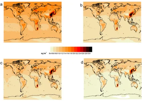
2.4 Surface Hg distribution

The modelled surface layer TGM concentration, averaged over the two year simu-lation period (2008-2009), is shown in figure 2.4.1. The figure shows the four vari-ations of the chemical mechanism which were employed. The latitudinal variation of surface TGM is shown in figure 2.4.2 which shows the results from the different redox combinations and also includes the results from the 8 and 12-month lifetime tracer experiments. The model reproduces the observed surface TGM concentra-tion gradient (>20%) between the Northern and Southern Hemisphere, indepen-dently of the chemical mechanism or the decay time adopted. This is an improve-ment on the previous version of the model, and is due to the revised treatimprove-ment of oceanic emissions compared toJung et al. [55]. It is clear from figures 2.4.1 and 2.4.2 that only the Base mechanism reproduces the typical mean background con-centration values of TGM of around 1.1 - 1.3 ng m−3in the Southern and of 1.5 - 1.7 ng m−3in the Northern hemisphere [63]. Of the tracer simulations the

(42)

12-Figure 2.4.1: Geographical distribution of Total Gaseous mercury (TGM)

surface concentration (ng/m3_{) as resulted by using different full chemistry}

mechanism: a) Base, b) Base2, c) Base4, d) Base3. Model values are annually averaged for the simulation period (2008-2009).

(43)

Figure 2.4.2: Hemispherical gradient of total gaseous mercury (TGM) as

resulted by using different full chemistry mechanism. Model data are averaged longitudinally for the 2008-2009 simulated period.

(44)

month lifetime simulation comes closest to reproducing the observed TGM val-ues and variation. The addition of Hg oxidation by NO3lowers the TGM surface

concentrations significantly at all latitudes, and the values of around 0.7 ng m−3 in the Southern and of 1.1 ng m−3 in the Northern hemisphere are not realistic. These values are comparable with the concentrations obtained from the 8-month lifetime tracer experiment.

The simulation Base4 with no gas phase OH oxidation and no aqueous phase reduction, with oxidation by O3+ NO3shows very similar surface concentrations

to the Base2 model. As the Base2 simulation includes the reactions with OH and HO2in addition to those with O3+ NO3, it appears that the OH and HO2reactions

have roughly equal but opposite effects on the TGM concentration. However this effect will vary with time and location as the distributions of OH and HO2differ

over space and time.

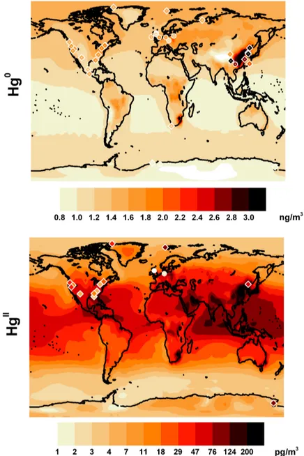
The form of the latitudinal variation (figure 2.4.2) obtained in the tracer exper-iment simulations is quite different from those obtained using the model’s chem-istry mechanisms due to the fact that the “decay” of Hg0to HgIIis assumed to be both temporally and geographically uniform, which is not a true reflection of the actual distribution of atmospheric oxidants. Figure 2.4.3 shows the average latitu-dinal distribution of the Hg0_{surface concentrations, and the 1}st_{to 99}th_percentile range(shaded area) of modelled value at each latitude. The Base model annual average was compared with the annual average Hg0_{surface observations from 35}

global sites. Observation data include those published in [119] plus additional data collected by sites belonging to EMEP programme. Where it was possible averages for the same years as the simulations were used (circles in figure 2.4.3), the other data shown (crosses) was collected over the period between 1995-2009. Figure 2.4.4 (top panel) reports the geographical distribution of the same observa-tions and model data. The model reproduces the spatial distribution of the Hg0

ob-servations,with the peak model variability in the Northern Hemisphere matched by the peak in the range of the observations. The high variability of TGM

(45)

con-Figure 2.4.3: Averaged latitudinal distribution of air concentrations of Hg0

as simulated by base Model. Red shadowed area represents the 1st _{to 99}th

per-centile range of the longitudinal variation. Annually averaged measurements are also reported: circles indicates measurements collected during the same

years of the simulation period. Observations include those used by [119] plus

(46)

Figure 2.4.4: Spatial distribution of annually averaged air concentrations of

Hg0 _{and Hg}II _{. The background model simulated data and the measurements}

for Hg0 _{are the same of Figure 2.4.3. Hg}II _{observations include those used by}

(47)

Figure 2.4.5: Mean seasonal variations of TGM at northern mid-latitudes.

Observations are annual means averaged over 6 EMEP sites. Shadowed area indicates the standard deviation for observations.

centration at around 30 degree south, and caused by the peak in the South Africa, is due to an overestimation of Hg emissions in the region [18]. The global spatial correlation (by mean of the Pearson’s r) is 0.7 with a slope of 0.85 and a normalised mean bias of -7% , in line with other model studies [49]

Figure 2.4.5 shows the comparison between simulated and observed monthly averages of TGM surface concentrations observed at Northern mid-latitudes sites (40-60◦). The Base run compared with the observations has a normalised mean bias of 16%, and the correlation (Pearson’s r) between them is 0.8. Using oxidation mechanism other than the Base gave poorer results. Interestingly the simulation in which oxidation by OH was not included gave particularly poor results, and correlation coefficient of just 0.1. In fact, observations show a minimum in the late

(48)

summer period in measurements. This minimum, well reproduced by the model, is attributed to oxidation of Hg by OH, and has been reported in previous modeling studies [49,98].

2.5 Hg Ocean Evasion

Recently a number of papers focused on the estimation of Hg0_{evasion from oceans}

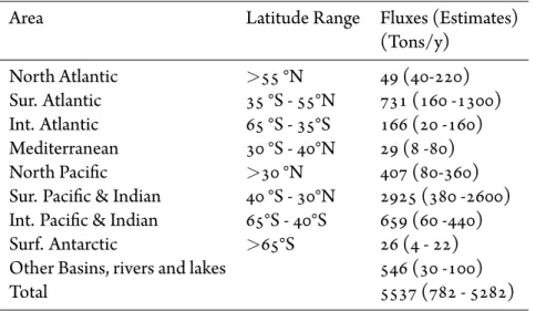
[67,96,99,102,111,115] have been published. Figure 2.5.1 (a) shows the global distribution of the simulated annual Hg0ocean emissions. The largest fluxes oc-cur in tropical regions where a combination of warm temperatures and relatively strong winds cause higher evasion rates. The mean Hg0emission flux for the ocean in tropical zones is between 0.7 and 1.5 μg m−2month−1(Figure 2.5.1 (b)) and displays the largest seasonal variability at±15 degrees, reflecting the seasonal mi-gration of the Intertropical Convergence Zone (ITCZ)[83,108]. Around the equa-tor there is an evasion minimum, and also a reduced seasonal variability due to the generally light winds in this area (the so-called Doldrums) [24]. Outside the trop-ics region, emissions from the northern hemisphere oceans show little seasonal variation, except for the Arctic Ocean where the seasonal formation and loss of sea-ice play a role. The Southern hemisphere oceans, show generally greater an-nual Hg0emissions with respect to those in the North. Emissions are strong dur-ing the entire year with a moderate seasonal variation, emissions are particularly high between 40 and 50◦N, due to the strong westerly winds found here, known as the roaring forties [108]. The pattern of the latitudinal distribution of Hg0_ocean

flux is similar to that obtained by Strode et al. [111], whereas the absolute values are somewhat greater since in Strode et al. [111] the mean global ocean concentra-tions of DGM was 0.07 pM. In table 2.5.1 the simulated annual Hg0_{emissions from}

the different ocean basins for the period 2008-2009 are shown, with previous es-timates in parentheses (see Sunderland and Mason [115] and references therein). The total simulated oceanic flux of Hg0to the atmosphere, 5500 Mg yr−1, is at the at the high end of the range of previous estimates (800-5300 Mg yr−1) and is

(49)

com-Figure 2.5.1: (a) Global distribution of Hg0 _{fluxes from oceans surface.} Fluxes are annual mean values from the model simulation period. (b)

Latitu-dinal distribution of the oceanic Hg0 _{Flux, in different seasons, and the annual}

(50)

Table 2.5.1: Simulated annual fluxes from the ocean to the atmosphere for

the various ocean regions. Ranges (90% confidence intervals) of previously estimated fluxes are also reported.

Area Latitude Range Fluxes (Estimates)

(Tons/y) North Atlantic >55 °N 49 (40-220) Sur. Atlantic 35 °S - 55°N 731 (160 -1300) Int. Atlantic 65 °S - 35°S 166 (20 -160) Mediterranean 30 °S - 40°N 29 (8 -80) North Pacific >30 °N 407 (80-360)

Sur. Pacific & Indian 40 °S - 30°N 2925 (380 -2600) Int. Pacific & Indian 65°S - 40°S 659 (60 -440)

Surf. Antarctic >65°S 26 (4 - 22)

Other Basins, rivers and lakes 546 (30 -100)

Total 5537 (782 - 5282)

parable with the estimate of Selin et al. [99] of 5000 Mg yr−1. This difference in the magnitude of the ocean evasion, with respect to other modeling studies may be due to differences between the re-analysis data used by ECHMERIT (ECMWF era-interim) and that used in other models. Moreover it should be noted that these are the first Hg0_{ocean emission estimates carried-out using a global scale on-line}

model, that does not interpolate in any way the meteorological fields (in either time and space) used in the parametrised calculation of oceanic Hg0_fluxes.

2.6 Hg deposition

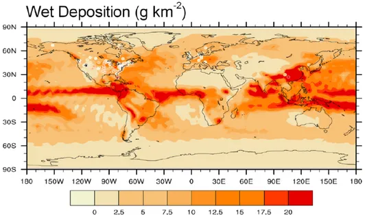
Figure 2.6.1 shows the averaged annual HgII_{wet deposition over the globe}

dur-ing simulation period as simulated by the Base model. The deposition is greatest over Asia, East Europe and over the eastern coast of North America, reflecting the largest anthropogenic emissions in these area.

(51)

Figure 2.6.1: Global distribution of wet deposition fluxes during the

simula-tion period

Wet Deposition over North America Stations making up the Mercury De-position Network (MDN, [39]) over North America collected samples on a weekly basis. In order to make an effective comparison between modelled and observed data only the stations that successfully collected data covering at least 3/4 of each year of the simulated period. Moreover any stations with no samples for a period longer than a month were excluded from the analysis. Figure 2.6.2 compares the re-sults of the Base model with data collected by the MDN network for the simulated period, 2008-2009. Simulations reproduce well fluxes observed by MDN network over the western US, where emission levels are the lowest. In the Eastern US where the highest anthropogenic emissions occur and indeed the measurements at MDN sites are also highest the model overestimates the observed deposition by almost a factor of 2 during the year. However this overestimation shows a distinct regional and seasonal variation. Figure 2.6.3 compares the simulated wet deposition with the observations in each seasons. The largest discrepancies between the model

(52)

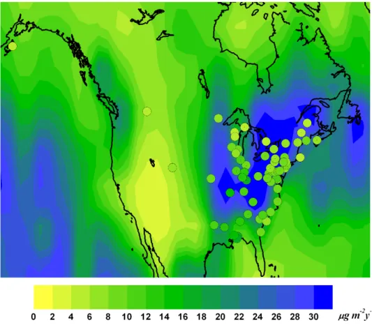
Figure 2.6.2: Annual Hg wet deposition fluxes over North America during

2008-2009 as simulated by base model. Overlaid circles show wet deposition observed during the same years by Mercury Deposition Network (MDN)

(53)

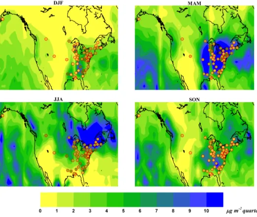
Figure 2.6.3: Seasonal Hg wet deposition fluxes over North America

aver-aged over 2008-2009 period, as simulated by base model (background) and observed by MDN sites (Circles).

(54)

and observations occur in the Spring and Summer and in the more industrialised north-eastern part of the US. Emissions of Hg from this area would mostly be de-posited locally and rapidly in the wetter autumn and winter months, however in Spring and Summer they are more likely to be transported further. However if the emissions have too high a proportion of HgIIthis could cause the model to over-estimate the deposition nearby to sources. Zhang et al. [140] have considered this possibility in a nested regional simulation within their global model.

Wet Deposition over Europe Figure 2.6.4 compares the results obtained by the Base model with annual wet deposition data collected by European Monitor-ing and Evaluation Programme (EMEP) durMonitor-ing 2008-2009. As above sites with at least 75 % of data available for each year of simulation period were used for the comparison. The highest wet deposition fluxes simulated by the model (the Base redox mechanism) are over the central and oriental area of the Europe, where the emissions from anthropogenic sources are the highest. The high wet deposition fluxes over some areas of the Atlantic Coast of Europe are due, at least in part to the frequent precipitation which occurs there. The model shows generally good geo-graphical agreement with the observations, especially over the coastal regions of Northern Europe, but tends to overestimate deposition fluxes in the more industri-alised regions of Central/Eastern Europe. Again this may be due to the proportion of oxidised Hg species in emissions, however due to the lack of monitoring stations in less industrial regions, particularly in Southern Europe it is not really possible to compare areas which are more and less directly impacted by local sources.

2.6.1 Global Hg Budget

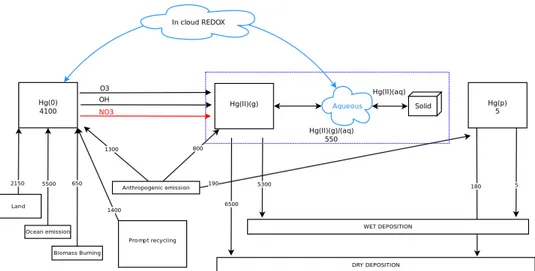
Figure 2.6.5 shows the global budget of the Hg as simulated by our Base model considering the updated emissions.

As described in sections 2.2.1 and 2.5 the anthropogenic and ocean emissions account for 2300 and 5500 Mg y−1. Terrestrial primary emissions from biogenic

(55)

Figure 2.6.4: Annual Hg wet deposition fluxes over Europe during 2008-2009

as simulated by base model. Overlaid circles show wet deposition observed during the same years by EMEP sites.

(56)

Figure 2.6.5: The total annual global Hg budget as derived from the base

model. Emission and deposition rates are given in Mg y−1. Inventories are in

Mg.

activities, evapotranspiration and forest fires account for 2800 Mg y−1close to other modelling estimates [99]. The prompt recycling of the previously deposited Hg species account for 1400 Mg y−1, greater than previously reported [59,99], re-flecting the greater total deposition. The total source of Hg to the atmosphere is 11800 Mg y−1, at the upper end of the range (6200-11200 Mg y−1) previously es-timated by GEOS-Chem [98,99] and slightly larger than the recent independent estimate of 9700 Mg y−1using CAM-Chem [59]. Almost all atmospheric Hg is removed as HgII

(g/aq). Dry deposition in ECHMERIT is somewhat greater

glob-ally than wet deposition, ( 6500 vs 5300 Mg y−1). The dry deposition of Hg0_is

negligible (less than 10 Mg y−1) due to the approach used for modelling the Hg0

deposition velocity (section 2.6). Other recent studies that suggest a much greater Hg0dry deposition flux, also found an atmospheric lifetime of total Hg of 0.5 and 0.69 year [59,99], much shorter than previously estimated (see for example Lind-berg et al. [63]. Although a shorter lifetime was supported by a decreasing trend in atmospheric Hg concentrations at many sites [101], ”other regions show an in-crease in the Hg levels”, suggesting possible not well-known regional reasons rather than a global trend [122].

(57)

The emitted inert and insoluble HgP_{, 190 Mg y}−1_{, is almost all removed by dry} deposition (180 Mg y−1. It should be recalled that in ECHMERIT much of the Hg associated with particulate matter is present as the soluble species HgII

(aq). The

total burden of Hg in atmosphere is 4650 Mg of which 4100 are Hg0, 550 HgII (g/aq)

(58)

Much of the content of this chapter appeared in [29]

3

A Model Study of Global Mercury

Deposition from Biomass Burning

Among all emissions source increased attention has also been given to Biomass Burning (BB) emissions [23,37,131], in trying to constrain the global budget of Hg as it cycles between environmental compartments. Friedli et al. [37] esti-mated Hg emissions from BB by combining outputs from global carbon emission models with Hg enhancement ratios and found that globally 675 (±240) Mg yr−1_, averaged over the period 1997-2006, is emitted from BB. As this figure is approx-imately one third of the yearly anthropogenic emissions of Hg to the atmosphere, it is clear that BB plays an important role in the Hg biogeochemical cycle. As con-trols on anthropogenic Hg emissions become stricter, proportionally the role of BB will increase, possibly substantially if the instances and extent of wildfires