0.8 Cop yedited by: MMP 1 2 3 4 5 6 7 8 9 10 11 12 13 14 15 16 17 18 19 20 21 22 23 24 25 26 27 28 29 30 31 32 33 34 35 36 37 38 39 40 41 42 43 44 45 46 47 2009, 1–22, iFirst
Population age structure and household portfolio choices in Italy
Marianna Brunetti
a,c,dand Costanza Torricelli
b,c∗aSEFEMEQ Department, University of Rome Tor Vergata, Via Columbia 2, 00133 Roma, Italy;bDepartment of Economics, University of Modena and Reggio Emilia, Via Berengario 51, 41100 Modena, Italy;cCEFIN (Center for Research in Banking and Finance), University of Modena and Reggio Emilia, Italy;dCHILD (Center for Household, Income, Labour and Demographic Economics), University of Turin, Italy
Based on the exceptional ageing of the Italian population, this paper aims to contribute to the current debate on population ageing and financial markets. To this end, we use the data taken by the Bank of Italy Survey of Household Income and Wealth over the period 1995–2006, and we analyse the average household portfolios in relation to age and net wealth (NW). Our analysis rests on a clustering of assets according to risk, which is different from the one used in Guiso and Jappelli (Guiso, L., and T. Jappelli. 2002. The portfolio of Italian households. In Household portfolios, eds. L. Guiso, M. Haliassos, and T. Jappelli. Cambridge: MIT Press). We find that age has affected financial choices of Italian households over the whole decade, but the portfolio age profile has significantly evolved over time with important differences across wealth quartiles. Overall, our analysis highlights a tendency towards a hump-shaped age profile of the allocation in risky assets for the most NW levels.
Keywords: population ageing; financial assets; household portfolio; survey data JEL Classification codes: D1; D91; J11
1. Introduction
Population ageing can really affect financial markets, since elderly people usually have lower Q1
saving rates and a higher average risk aversion. Thus, ageing brings about a progressive evolution of financial needs and investment requirements, which may in turn translate into changes in prices and returns of existing financial instruments (Poterba 2001 for US; Brunetti and Torricelli 2008 for Italy) and in the need for new ones (Fornero and Luciano 2004). A lively debate on the financial effects of ageing is ongoing among both academics and practitioners, and has originated a vast literature constituted by both theoretical and empirical contributions. The latter, in particular, have increased over the last decade, also fostered by the increasing availability of suitable survey data sets. Part of this empirical literature has focused on the effects that demographic dynamics might have at a macro-economic level (i.e. on growth or savings and interests rates): among others see Demery and Duck (2006), Miles (1999), Oliveira Martins et al. (2005), Visco (2002) and Yakita (2006). On the other hand, a particular strand of the empirical literature has focused on the effects that ageing may have on financial asset returns and portfolio allocations: see, Brooks (2000, 2002), Davis and Li (2003), Ameriks and Zeldes (2004), Geanakoplos, Magill, and Quinzii (2004), Goyal (2004) and Poterba (2001, 2004). The basic idea underlying most papers is the life-cycle hypothesis, according to which individual saving behaviour and portfolio choices vary over
∗Corresponding author. Email: [email protected] ISSN 1351-847X print/ISSN 1466-4364 online
© 2009 Taylor & Francis
DOI: 10.1080/13518470903075961
http://www.informaworld.com
48 49 50 51 52 53 54 55 56 57 58 59 60 61 62 63 64 65 66 67 68 69 70 71 72 73 74 75 76 77 78 79 80 81 82 83 84 85 86 87 88 89 90 91 92 93 94
the life cycle. As for the latter in particular, early models for the life-cycle portfolio theory1 basically suggests that the allocation in risky assets should decrease with age, a rule that has been often suggested by professional consultants too (Malkiel 1996) as the (100–age)% rule. However, this prescription is in contrast with the most empirical evidence (Curcuru, Heaton, and Lucas 2007; Gomes and Michaelides 2005) and since the late 1990s, the theoretical literature has been including features of realism, and specifically, the consideration of back-ground risk that generally imply an hump-shaped age pattern for the allocation in risky assets (Benzoni, Collin-Dufresne, and Goldstein 2007).
The existing literature is far from being homogeneous in terms of objectives, methodology and results. Focusing on the empirical literature on household portfolio choices,2we have two main objectives as follows: the study of the asset allocation choice and the study of the participation choice, i.e. the decision of whether or not to invest in risky assets such as stocks. According to the main objective, a different methodological approach can be taken: for asset allocation analyses a descriptive approach that elaborates and interprets trends in survey data can be used, whereas an econometric approach that essentially runs time series or panel data analyses is applied in the analysis of the variables determining the participation decision. In some papers, the econometric approach is further used to estimate the percentage invested in risky assets either unconditionally or conditionally on the participation decision.3It has to be stressed, however, that the descriptive
approach, although quantitatively less sophisticated, allows to go beyond the focus on the stock holding decision, since it describes the whole asset allocation and to get an inspection over its determinants.
In terms of outcomes, both descriptive and econometric analyses support an apparent hetero-geneity in terms of stock market participation and asset allocations as shown by studies for different countries (Guiso, Haliassos, and Jappelli 2002 for US, UK, Italy, Germany and Netherlands). Three main results emerge from the empirical literature: low stock-market participation, scarce diversifi-cation and a life cycle of household portfolios that display a hump shape, whereby the investment in stocks peaks at Middle Ages. Particularly interesting is the evidence on asset allocation, which, although disparate, when supporting a hump-shaped age pattern contradicts most portfolio models and popular financial advice, suggesting an investment in stock decreasing with age.
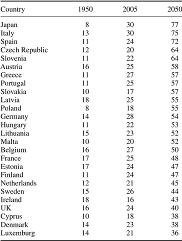
In the latter connection, the portfolio allocation of Italian household deserves further investi-gation, since Italy displays an exceptional ageing of the population as highlighted in Table 1. The table ranks countries according to the expected value for this demographic indicator in 2050: the process of population ageing seems to affect quite strongly several of the new EU members, and, in particular, Slovenia and Czech Republic,4 but Italy is the sole country whose projections are as high as that of Japan.
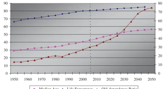
The peculiarity of the Italian case is apparent in Figure 1: since the mid of last century, both Italian median age and life expectancy at birth have remarkably increased, and the old depen-dency ratio has more than doubled. As for the future, these dynamics are going to be even more pronounced: according to UN projections in fact by 2050 in Italy, there will be around 75 retired for every 100 working people.
Guiso and Jappelli (2002) analyse the Italian household portfolio evolution using data from the 1989, 1991, 1993, 1995 and 1998 editions of the Bank of Italy Survey of Household Income and Wealth (SHIW). Then, to single out main determinants, they group financial assets into three main categories as follows: safe (e.g. bank accounts), fairly safe (e.g. T-Bills and similar) and risky (e.g. stocks, long-term government bonds and mutual funds), and use this classification for both the descriptive and econometric investigation. As for the former, the share of safe and fairly safe assets reduced (from 45.7 to 25% of total financial wealth) and that of risky assets increased (from
95 96 97 98 99 100 101 102 103 104 105 106 107 108 109 110 111 112 113 114 115 116 117 118 119 120 121 122 123 124 125 126 127 128 129 130 131 132 133 134 135 136 137 138 139 140 141
Table 1. Old dependency ratios.
Country 1950 2005 2050 Japan 8 30 77 Italy 13 30 75 Spain 11 24 72 Czech Republic 12 20 64 Slovenia 11 22 64 Austria 16 25 58 Greece 11 27 57 Portugal 11 25 57 Slovakia 10 17 57 Latvia 18 25 55 Poland 8 18 55 Germany 14 28 54 Hungary 11 22 53 Lithuania 15 23 52 Malta 10 20 52 Belgium 16 27 50 France 17 25 48 Estonia 17 24 47 Finland 11 24 47 Netherlands 12 21 45 Sweden 15 26 44 Ireland 18 16 43 UK 16 24 40 Cyprus 10 18 38 Denmark 14 23 38 Luxemburg 14 21 36
Note: Old dependency ratio is defined as the ratio of people aged 65 or more over the total active population.
Data source: United Nations Population Prospects.
around 16 to around 47%). According to the authors, several ‘macro-economic’ circumstances may have taken part in these changes: the decline in short-term bonds nominal yield coupled with the increase in equity returns that characterized the entire 1990s, the liberalization of capital market, which encouraged international diversification starting from 1989, the birth of mutual funds in 1984 and the privatization in 1992 that most likely boosted market capitalization, as well as the social security reforms that fostered the development of life insurances and pension funds. Nevertheless, specific household features, such as wealth, education and age may also have affected these changes in the portfolio allocation. Guiso and Jappelli (2002) thus focus on the 1989–1995 period and study whether or not these factors played a role in determining the riskier portfolio allocation. Overall, the econometric analyses, based on cross-sectional and panel data, suggest that age together with wealth and education may have a substantial influence on the participation decision, while once this decision is taken these factors only slightly affect the final portfolio allocation.
Guiso and Jappelli (2002) focus on a time period, end-1980s to mid-1990s, in which several changes had already occurred but many others still had to take place, both at an institutional and at a financial market level. As for the former in fact, the Italian pension system underwent a series of interventions, the most important being the 1995 reform, known as the Dini reform. The
142 143 144 145 146 147 148 149 150 151 152 153 154 155 156 157 158 159 160 161 162 163 164 165 166 167 168 169 170 171 172 173 174 175 176 177 178 179 180 181 182 183 184 185 186 187 188 0 10 20 30 40 50 60 70 80 90 1950 1960 1970 1980 1990 2000 2010 2020 2030 2040 2050 0 10 20 30 40 50 60 70 80
Median Age Life Expectancy Old-dependency Ratio
Note: values for median age and life expectancy can be read on the left scale, those for old-dependency ratio on the right-hand-side scale.
Data Source: United Nations Population Prospects.
Figure 1. Main demographic measures in Italy: Evolution and forecast.
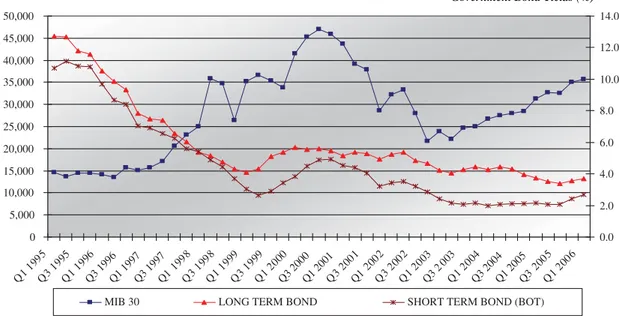
main aims were to set-up a stronger link between pension benefits and lifetime contributions, to reduce the replacement rate and, in order to face the lengthening of life time span, to progressively increase the retirement age. For an in-depth description of each pension system reform part of the restructuring process of the Italian pension system see, among others, Baldacci and Tuzi (2003) and Brugiavini and Galasso (2003). As for the financial market, developments both in the government bond market and in the stock market, including the well-known 2000 boom, are apparent from Figure 3.
We thus believe that Italy during the period 1995–2006 represents an interesting case study in order to test whether age is a relevant factor influencing household’s portfolio not just in terms of participation decision but also in terms of allocation decision. More specifically, we aim to assess if and how Italian household portfolios have reacted to these changes and to test whether their choices are consistent with the theoretical suggestion provided by classical (i.e. risky asset holdings decreasing with age) or some of the more recent portfolio choice models (i.e. hump-shaped risky asset holdings).
To this end, we use data taken from the Bank of Italy SHIW and employ the descriptive approach, since it allows to get inspection into the dynamics of the Italian households’ portfolios along many directions and specifically to assess to what extent changes can be traced back to demographic factors. Our analyses differ from the descriptive study in Guiso and Jappelli (2002) in three extents: first, we consider a subsequent period of time characterized by a different economic and institutional setting; second, we take financial market changes into account and propose a different financial asset sorting according to their risk profiles and third, we refine the analyses by separating households into both age classes and net wealth (NW) percentiles, which allow testing the robustness of age effect on financial choices.
The paper is structured as follows. Section 2 illustrates the methodology and data set. The empirical descriptive analyses on household portfolios in Italy are presented in Section 3. Section
189 190 191 192 193 194 195 196 197 198 199 200 201 202 203 204 205 206 207 208 209 210 211 212 213 214 215 216 217 218 219 220 221 222 223 224 225 226 227 228 229 230 231 232 233 234 235
4 highlights the novelty with respect to a previous analysis for Italy. The final section concludes. The appendix discusses the clustering of assets made in this study according to the risk profile and compares it with Guiso and Jappelli (2002).
2. Data set and methodology
Data are taken from the Historical Archive of the Bank of Italy SHIW (HA-SHIW) and span over the 1995–2006 decade with six waves available: 1995, 1998, 2000, 2002, 2004 and 2006. Beside socio-economic information, the data set offers a detailed picture of the financial portfolio held by the interviewed households, as it provides the amounts (expressed in Italian lira until 2000 and in euro thereafter) invested in a variety of financial assets. In order to allow a better comparability across time, we translate these amounts into percentages over total financial assets held5and we group assets into different classes according to their risk profiles. In the risk classification, the focus is centred on two kinds of risks only: credit and market risk.
As for the former, we distinguish two different levels. The ‘lower’ level is assigned to financial assets issued by both the domestic sovereign (i.e. Italian government) and by banks, securities firms and co-operatives, based on the always more stringent supervising regulations introduced by the Basel II Accord and of the several security provisions provided for by the law specif-ically aimed to make banks and financial systems as safe as possible. The ‘higher’ level is instead associated with all the assets issued by the remaining agents, basically corporations. Foreign activities are treated separately as the amounts provided by the HA-SHIW do not distin-guish non-residents issuers so that a more precise credit-risk classification for these assets is not possible.
As far as market risk is concerned, three main types are considered, i.e.: exchange rate risk, which concerns the foreign activities only, interest rate risk, associated with all bonds securities, and price risk, associated with stocks and shareholdings. In addition, a fourth category, referred to as ‘mixed’, is created for investments where bonds (interest rate risk) and stocks (price risk) are mixed together (Table 2). Six main financial asset groups are thus identified:6
(1) Deposits: lower credit risk and no market risk
(2) Government bonds: lower credit risk and interest rate risk (3) Corporate bonds: higher credit risk and interest rate risk (4) Managed investments: lower credit risk and mixed market-risk (5) Stocks: higher credit risk and price risk
(6) Foreign assets: exchange rate risk
Two observations are in order. First, in the following analyses, values for life insurances and pension funds will be presented separately, as the focus of this study makes their single evolu-tions particularly interesting. Second, following Guiso and Jappelli (2002) in a second stage of the analysis, financial assets are further grouped into three risk categories: ‘safe’, ‘fairly safe’ and ‘risky’. The definition of these risk categories, however, differ slightly from the previous study since fairly safe assets include government bonds and managed investments, and risky assets comprise corporate bonds, stocks and foreign activities (see Table 2 and Table A1 in the appendix).
The analysis is articulated in three phases. As a first step, the evolution of the average portfolio of Italian households is observed across all the five waves considered in order to highlight the main features of the average Italian household portfolio and, in particular, its low degree of
236 237 238 239 240 241 242 243 244 245 246 247 248 249 250 251 252 253 254 255 256 257 258 259 260 261 262 263 264 265 266 267 268 269 270 271 272 273 274 275 276 277 278 279 280 281 282
Table 2. Financial assets classification, by credit and market risk. Market
Credit – Interest rate Mixed Price Exchange rate
Lower Current accounts Postal bonds REPO
Savings deposits Short-term
government bonds
Investment funds
Postal deposits Bonds Personal assets
managements Certificate of deposits Long-term government Pension funds
Cooperative loans Bonds Life insurances
Health-insurances Other insurances
Higher Corporate bonds Stocks
SRL shares Partnership
– Foreign assets
Note: Shaded cells indicate comparable risk profiles; light grey denotes safe assets; more intense grey indicates fairly safe assets; and dark grey gathers the risky ones.
diversification and to examine whether and to what extent it has actually changed over the last decade. Second, in order to depict a possible age effect on the Italian household portfolio, the households are then divided into six age classes (<30, 30–39, 40–49, 50–59, 60–69 and >70) and for each of them the average portfolio is examined. The placement in the age classes is made according to the age of the head of the household.7Third, since household financial choices are
affected by many other elements besides age (e.g. overall economic conditions), we study the dependence of the age effect on overall wealth. Households are thus divided into three groups according to their NW, defined as the sum of real and financial activities net of the financial liabilities.8More specifically, we analyse separately households under the 25th percentile, between the 25th and the 75th and between the 75th and 95th (the top 5% richest households have been excluded because of their peculiar economic conditions, see Table 3). In short, the last step of our analysis consists in examining the average portfolio allocation of all the interviewed households by age classes and NW and to observe their evolution across the last decade.
Table 3. NW percentiles boundaries by SHIW wave.
In millions lira In thousands euro
Percentile 1995 1998 2000 2002 2004 2006
25th 58.10 60.00 70.50 41.00 43.00 48.50
50th 185.94 202.00 215.00 126.00 152.00 170.66
75th 365.05 381.81 421.00 250.00 285.80 323.20
95th 961.34 1127.30 1224.14 695.68 727.00 855.00
283 284 285 286 287 288 289 290 291 292 293 294 295 296 297 298 299 300 301 302 303 304 305 306 307 308 309 310 311 312 313 314 315 316 317 318 319 320 321 322 323 324 325 326 327 328 329
3. New evidence on ageing and Italian households portfolio choices
The data presented in the previous section can be used in the analysis of household portfolios along three directions: (i) ‘vertically’, the data highlight the differences in financial allocations of households belonging to the same age class but with different NW; (ii) ‘horizontally’, they depict the possible effect of age on the household’s financial portfolio, since the allocations are compared across different age classes but comparable economic conditions; and (iii) ‘transversally’ across the SHIW waves, they highlight whether the average portfolio allocation of households of the same age class and NW quartile has modified or not, depicting in this way a possible time effect. Specifically for the Italian case, this intertemporal reading can be particularly interesting as it might reveal ‘indirect’ effects of ageing, e.g. those induced by the several radical reforms brought to the social security system during the last decade and called for by the striking ageing of the Italian population.
3.1 The average household portfolio in 1995–2006
As a first step, the survey data are used to determine the average portfolio of Italian households in each of the six waves. From this preliminary inspection, the scarce degree of diversification of Italian household portfolios immediately emerges: during the whole decade in fact Italian households hold on average around 70% of their financial wealth in deposits (Figure 2). This peculiarity was already stressed by Guiso and Jappelli (2002) for the period 1989–1995: ‘the portfolios of Italian households span few assets. A large fraction of the sample holds very few types of financial instruments and tends to concentrate wealth in safe assets’.9
Table 4 reports the average shares invested by Italian households in each financial asset category for each wave between 1995 and 2006 as from the HA-SHIW.
330 331 332 333 334 335 336 337 338 339 340 341 342 343 344 345 346 347 348 349 350 351 352 353 354 355 356 357 358 359 360 361 362 363 364 365 366 367 368 369 370 371 372 373 374 375 376
Table 4. Average household portfolios by SHIW wave.
Financial assets 1995 1998 2000 2002 2004 2006 Deposits 65.15 73.46 67.78 71.45 74.57 74.23 Government bonds 20.94 8.74 8.91 7.27 7.15 7.73 Corporate bonds 0.97 1.79 2.08 2.53 2.53 2.84 Stocks 5.68 8.44 10.81 9.50 8.53 8.49 Managed investments 1.34 2.78 4.23 3.93 3.15 2.54 Life insurances 4.54 3.50 3.98 3.70 2.41 2.42 Pensions funds 1.26 1.12 1.90 1.27 1.32 1.49 Foreign activities 0.12 0.16 0.30 0.36 0.33 0.26
Note: For each asset, the table reports the weighed average percentage over total financial asset (using sample weights as from HA-SHIW).
As said, the share of deposits has remained almost unchanged at around 70% over the entire decade. By contrast, the incidence of government bonds has drastically reduced: in 2006, their share was only one-third of the average value observed a decade before. Most likely, this change can be ascribed to the drastic reduction of Italian government bonds yields (Figure 3). In fact, after a first recover around 2000–2001, the yields on government bonds kept decreasing, although more gradually, during all the following years. On the other hand, investments in corporate bonds have progressively increased, especially starting from 1998. The privatization process in this case might have played an important role: although started in 1992, in effect, the peak of privatizations occurred at the end of 1990s.10
Survey data prove that also the average investment in stocks has undergone several changes, which in large part occurred according with the major market fluctuations of the last decade. Stock
0 5,000 10,000 15,000 20,000 25,000 30,000 35,000 40,000 45,000 50,000 Q1 1 995 Q3 1 995 Q1 1 996 Q3 1996Q1 1997Q3 1997Q1 199 8 Q3 1 998 Q1 1 999 Q3 1 999 Q1 2 000 Q3 2000Q1 2001Q3 200 1 Q1 200 2 Q3 2 002 Q1 2 003 Q3 2 003 Q1 2 004 Q3 2004Q1 2005Q3 200 5 Q1 2 006 0.0 2.0 4.0 6.0 8.0 10.0 12.0 14.0
MIB 30 LONG TERM BOND SHORT TERM BOND (BOT)
M ib 30 Government Bond Yields (%)
Note: values for Mib30 (left scale) are in index points while government yields (right scale) are percentages. Data Source: Datastream
377 378 379 380 381 382 383 384 385 386 387 388 389 390 391 392 393 394 395 396 397 398 399 400 401 402 403 404 405 406 407 408 409 410 411 412 413 414 415 416 417 418 419 420 421 422 423
share has progressively increased until 2000, up to more than doubling in 5-year time, and then it has shrunk again, along with the contraction of Italian stock market (see Mib30 trend in Figure 3). The same holds for managed investments, whose share increase from 1.34% in 1995 to 4.23% in 2000 and then shrink back to 2.54% in 2004, although their weight has overall increased during the decade under analysis.
As far as precautionary savings are concerned, the share invested in life insurances has pro-gressively reduced (from 4.54% in 1995 to 2.42% in 2006). The average share of pension funds shows a small increase around 2000: in fact, although introduced in 1995, they were enforced by appropriate laws only a couple of years later. Nevertheless, the launch of this form of comple-mentary social security does not seem to have worked particularly well in Italy: after the initial increase, the pension fund share has reduced back to around 1.5%, i.e. only slightly higher than the value recorded in the year of their introduction. Furthermore, although during the decade the gap between life insurances and pension funds has progressively thinned, the former are still somehow preferred with respect to the latter.
3.2 The average portfolio by age
In order to analyse the existence and the feature of an age effect on portfolio allocations, we first analyse the average household portfolios by age class of the head of the household for every wave available for the last decade in the HA-SHIW.
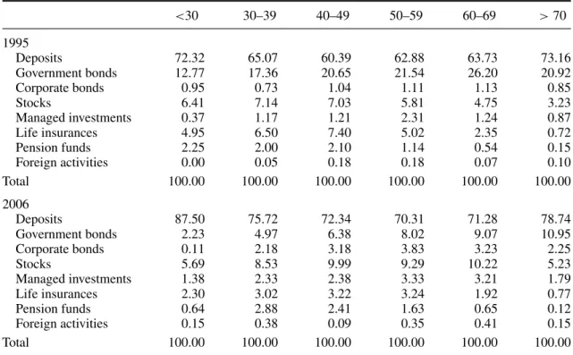
For reasons of space in Table 5, we report only the two extremes of the sample that allow us to highlight that an age effect does exist but it has considerably evolved over time (intermediate
Table 5. Average portfolio shares by age class, 1995 and 2006.
<30 30–39 40–49 50–59 60–69 > 70 1995 Deposits 72.32 65.07 60.39 62.88 63.73 73.16 Government bonds 12.77 17.36 20.65 21.54 26.20 20.92 Corporate bonds 0.95 0.73 1.04 1.11 1.13 0.85 Stocks 6.41 7.14 7.03 5.81 4.75 3.23 Managed investments 0.37 1.17 1.21 2.31 1.24 0.87 Life insurances 4.95 6.50 7.40 5.02 2.35 0.72 Pension funds 2.25 2.00 2.10 1.14 0.54 0.15 Foreign activities 0.00 0.05 0.18 0.18 0.07 0.10 Total 100.00 100.00 100.00 100.00 100.00 100.00 2006 Deposits 87.50 75.72 72.34 70.31 71.28 78.74 Government bonds 2.23 4.97 6.38 8.02 9.07 10.95 Corporate bonds 0.11 2.18 3.18 3.83 3.23 2.25 Stocks 5.69 8.53 9.99 9.29 10.22 5.23 Managed investments 1.38 2.33 2.38 3.33 3.21 1.79 Life insurances 2.30 3.02 3.22 3.24 1.92 0.77 Pension funds 0.64 2.88 2.41 1.63 0.65 0.12 Foreign activities 0.15 0.38 0.09 0.35 0.41 0.15 Total 100.00 100.00 100.00 100.00 100.00 100.00
Note: For each asset, the table reports the weighed average percentage over total financial asset (using sample weights as from HA-SHIW).
424 425 426 427 428 429 430 431 432 433 434 435 436 437 438 439 440 441 442 443 444 445 446 447 448 449 450 451 452 453 454 455 456 457 458 459 460 461 462 463 464 465 466 467 468 469 470
waves are available upon request)11. A comparative inspection of the data shows that in both waves the allocations are not constant across age, but although the levels are always different, which is justified by different market and institutional settings at the two extremes of the decade, the age pattern is similar in the two waves only for some assets (e.g. deposits, managed investments, life insurances) but quite different for government bonds and especially for the most risky investment, i.e. stocks.
While more stable results are consistent with the idea of the middle-aged taking up more risk, the reduced holdings in the government bond can be explained by the supply side (Figure 3) and the most notable result remains that for that of stocks, which in the literature represent the most con-troversial and debated case. In fact, in 1995 we obtained a decreasing pattern, which is consistent with the professional (100–age)% rule. However the validity of this rule been contrasted in the lit-erature since the 1990s by models accounting for background risks and obtaining the hump shape for stock holding as the optimal prescription. This is precisely the pattern we obtained in 2006.
In order to get more insight aggregate into the dynamics of asset allocation decision across age classes, it is necessary to take into account one of the aspects that, besides age, most significantly affects household portfolios, i.e. the household overall economic situation. This is the analysis we perform in the next section where the role of NW in portfolio allocations is analysed in connection with age.
3.3 The average portfolio by age and NW
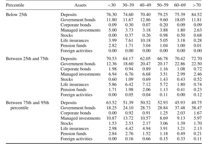
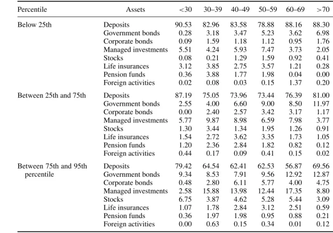
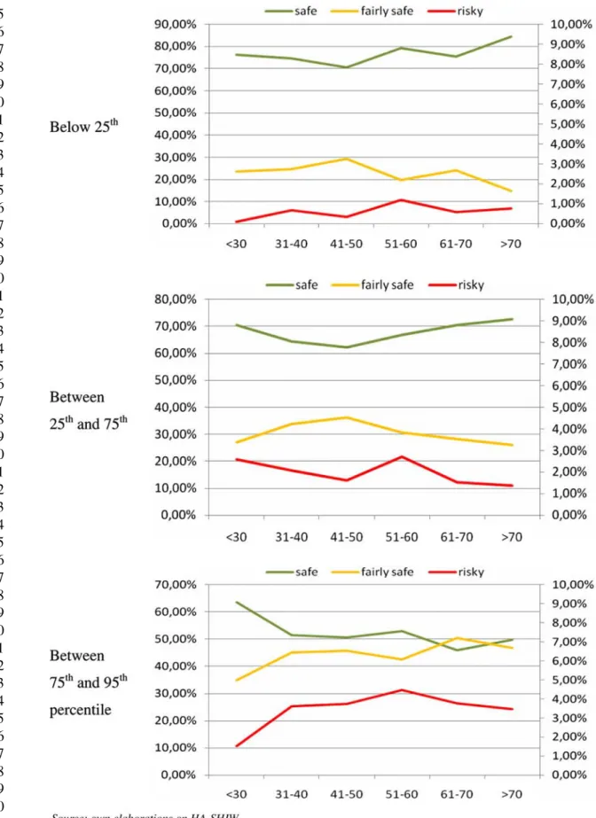
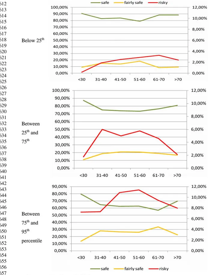
Tables 6 and 7 report the average household portfolios by age class in different NW quartiles (first, two central ones, last) for the 1995 and 2006 waves, respectively,12and highlights that NW plays a focal role in household portfolio choices. Figures 4 and 5 depict portfolio allocation by age class, NW and riskiness (defined according to Table 2).
A comparative inspection of tables and charts allows to draw some conclusions on the level and the age pattern of each asset class or riskiness class in connection with NW. First, as for the level, the degree of diversification increases with NW in both waves, whereby households below the first NW quartile have quite low degrees of diversification and riskiness. In fact, in 1995 all age classes held on average 70–80% of their financial wealth in deposits. The remaining was invested mainly in government bonds and, to a lesser extent, in managed investments and precautionary savings. This is even more striking in 2006, with the sole difference that managed investments (around 2–7% depending on the age class) tend to prevail on government bonds (0–7%). Intermediate NW households, i.e. between the first and the third quartiles, progressively diversify more and take up more risk. In both waves, the share of deposits reduces almost 10% points, while both government and corporate bonds become more relevant: note, however, that while in 1995 government bonds reach the 12–23% of the total financial wealth, in 2006 they range between 3% and 12%, a fact that can be explained by a change in the market conditions in Italy (Figure 3). The incidence of managed investments also overall increases in the intermediate household portfolios, reaching for relatively younger households peaks of 7% in 1995 and of 10% in 2006. Besides, the weights of the pre-cautionary savings basically remain unchanged: in both waves, in fact, the aggregate share of life insurances and pension funds does not diverge too much from the first quartile. The highest degree of diversification and riskiness is reached by the portfolios of households above the third quartile. Financial resources are in this case drained from deposits and directed towards riskier activities, such as stocks but especially managed investments that generally increase the most moving upward across NW, reaching for richer households in 2006 also 7–14% of the total financial wealth.
471 472 473 474 475 476 477 478 479 480 481 482 483 484 485 486 487 488 489 490 491 492 493 494 495 496 497 498 499 500 501 502 503 504 505 506 507 508 509 510 511 512 513 514 515 516 517
Table 6. Average portfolio by NW quartile and age class, 1995.
Percentile Assets <30 30–39 40–49 50–59 60–69 >70 Below 25th Deposits 76.30 74.60 70.40 79.25 75.39 84.52 Government bonds 11.80 11.67 12.86 9.60 18.05 11.81 Corporate bonds 0.09 0.30 0.07 0.20 0.09 0.09 Managed investments 5.00 3.73 3.18 3.88 1.80 2.63 Stocks 0.00 0.37 0.26 0.98 0.50 0.68 Life insurances 3.99 7.61 10.18 5.05 3.18 0.28 Pension funds 2.82 1.71 3.04 1.04 1.00 0.01 Foreign activities 0.00 0.00 0.00 0.00 0.00 0.00
Between 25th and 75th Deposits 70.53 64.17 62.05 66.78 70.42 72.70
Government bonds 12.36 18.60 20.47 20.17 22.86 22.50 Corporate bonds 1.98 0.94 0.89 1.16 1.08 0.72 Managed investments 6.94 6.76 6.68 3.51 2.99 2.46 Stocks 0.60 1.09 0.69 1.43 0.43 0.52 Life insurances 5.86 6.42 7.12 5.72 1.80 0.74 Pension funds 1.71 1.98 2.06 1.13 0.41 0.23 Foreign activities 0.00 0.05 0.04 0.11 0.00 0.12 Between 75th and 95th percentile Deposits 63.52 51.39 50.52 52.93 45.93 49.75 Government bonds 18.25 24.10 28.73 28.84 37.48 38.47 Corporate bonds 0.00 0.92 0.91 1.25 2.03 1.67 Managed investments 10.87 13.72 10.57 8.69 9.13 5.97 Stocks 1.53 2.53 2.17 3.06 1.39 1.70 Life insurances 2.98 4.42 4.94 3.91 3.21 2.13 Pension funds 2.84 2.76 1.52 1.18 0.49 0.21 Foreign activities 0.00 0.16 0.66 0.15 0.33 0.11
Note: For each asset, the table reports the weighed average percentage over total financial asset (using sample weights as from HA-SHIW).
Second, also the age pattern of asset allocations changes with NW, but the interesting result here is that there are substantial differences between the two waves. From Figure 4, it clearly appears that below the first NW quartile, there is no apparent life-cycle pattern in either riskiness class. Moving to the intermediate NW household, we observe a typical, although not much pronounced life-cycle pattern of safe (U shape) and fairly safe investments (inverted U) and a mixed evidence for risky ones: it appears as if the (100–age)% rule at the age of 40 left room to the inverted U life-cycle pattern. In the highest NW quartile, although still not much pronounced, life-cycle patterns are observable for all riskiness class. In 2006 the picture changes quite clearly as it is noticeable from Figure 5. The typical U (for safe assets) and inverted U (for fairly safe and risky assets) life-cycle patterns appear already for the poorest households and become progressively more evident for the richer ones. Moreover, troughs (for safe assets) and peaks (for riskier assets), which are on the whole independent of age across quantiles in 1995, become age sensitive and tend to increase with age as we move from poorer to richer quartiles.13
Hence the question is: what has changed in the last decade, which can explain evidence that is more consistent with the theoretical models suggesting life-cycle asset allocations in 2006 than in 1995? Possible explanations rest on the market supply conditions, the institutional changes in the labour market and pension system and an increased financial awareness on behalf of the households. As for the former, the changes in the market certainly play a role: from the decreased profitability of government bonds to the importance of the stock market evolution that hit Italy
518 519 520 521 522 523 524 525 526 527 528 529 530 531 532 533 534 535 536 537 538 539 540 541 542 543 544 545 546 547 548 549 550 551 552 553 554 555 556 557 558 559 560 561 562 563 564
Table 7. Average portfolio by NW quartile and age class, 2006.
Percentile Assets <30 30–39 40–49 50–59 60–69 >70 Below 25th Deposits 90.53 82.96 83.58 78.88 88.16 88.30 Government bonds 0.28 3.18 3.47 5.23 3.62 6.98 Corporate bonds 0.09 1.59 1.18 1.12 0.95 1.76 Managed investments 5.51 4.24 5.93 7.47 3.73 2.05 Stocks 0.08 0.21 1.29 1.59 0.92 0.41 Life insurances 3.12 3.85 2.75 3.57 1.21 0.28 Pension funds 0.36 3.88 1.77 1.98 0.04 0.00 Foreign activities 0.02 0.08 0.03 0.15 1.37 0.20
Between 25th and 75th Deposits 87.19 75.05 73.96 73.44 76.39 81.00
Government bonds 2.55 4.00 6.60 9.00 8.50 11.97 Corporate bonds 0.00 2.40 2.57 3.42 3.17 1.17 Managed investments 5.77 9.87 8.98 6.59 7.98 3.77 Stocks 1.30 3.44 1.34 1.95 1.26 0.91 Life insurances 1.54 2.72 3.62 3.35 1.73 1.05 Pension funds 1.20 2.36 2.84 1.82 0.82 0.12 Foreign activities 0.44 0.17 0.09 0.41 0.15 0.02 Between 75th and 95th percentile Deposits 79.42 64.54 62.41 62.53 56.87 69.56 Government bonds 9.34 8.53 7.91 9.56 12.92 12.87 Corporate bonds 0.48 2.80 6.11 5.77 4.00 4.75 Managed investments 2.58 15.88 13.98 12.44 17.35 8.80 Stocks 6.75 3.87 4.62 5.28 5.44 3.09 Life insurances 1.07 1.78 2.84 3.12 2.51 0.59 Pension funds 0.36 1.97 1.98 0.95 0.88 0.21 Foreign activities 0.00 0.63 0.15 0.34 0.01 0.12
Note: For each asset, the table reports the weighed average percentage over total financial asset (using sample weights as from HA-SHIW).
(see Figure 3, the point is taken up in the next section in connection with Figure 8). At the same time, the 1995 pension reform in Italy has been producing effects afterwards, and these effects become apparent in producing life-cycle asset allocation in precautionary savings. Finally, both the market and the institutional changes just mentioned, and in particular, the less generous public pension system might have increased in the last decade the household awareness of the need to make a choice over the life cycle in relation to the age.14
4. A comparison with previous analyses for Italy
The results of this paper in the case of Italy call for a link with the comparable ones in Guiso and Jappelli (2002). As illustrated in the introduction, we consider a different period with only one wave overlap (1995) and a different asset clustering in term of riskiness (see appendix and Table A1). Moreover, Guiso and Jappelli (2002) use a different approach: when analysing the age effect on portfolio, they pool the 1989–1995 data and focus on risky assets sorted according to their own classification, when examining the wealth effect on portfolio, they sort households into wealth (financial plus non-financial activities) rather than NW quartiles so that, in contrast to the present paper, on one hand they include into the portfolio also non-financial assets, on the other they focus on the effect of wealth only. It follows that our results are not directly comparable with Guiso and Jappelli (2002) and, in order to detect to what extent they are determined by
565 566 567 568 569 570 571 572 573 574 575 576 577 578 579 580 581 582 583 584 585 586 587 588 589 590 591 592 593 594 595 596 597 598 599 600 601 602 603 604 605 606 607 608 609 610 611
612 613 614 615 616 617 618 619 620 621 622 623 624 625 626 627 628 629 630 631 632 633 634 635 636 637 638 639 640 641 642 643 644 645 646 647 648 649 650 651 652 653 654 655 656 657 658
659 660 661 662 663 664 665 666 667 668 669 670 671 672 673 674 675 676 677 678 679 680 681 682 683 684 685 686 687 688 689 690 691 692 693 694 695 696 697 698 699 700 701 702 703 704 705
706 707 708 709 710 711 712 713 714 715 716 717 718 719 720 721 722 723 724 725 726 727 728 729 730 731 732 733 734 735 736 737 738 739 740 741 742 743 744 745 746 747 748 749 750 751 752
753 754 755 756 757 758 759 760 761 762 763 764 765 766 767 768 769 770 771 772 773 774 775 776 777 778 779 780 781 782 783 784 785 786 787 788 789 790 791 792 793 794 795 796 797 798 799
Figure 8. Risky assets allocations across different waves and age classes: Comparison of the two risk classifications.
the different period rather than the different clustering, we have used the Guiso–Jappelli (GJ) definition and performed again the analyses of Section 3 over the decade 1995–2006.
For reasons of space and comparability, we report the outcomes, along the age and NW dimen-sions, for the two extreme waves in Figures 6 and 7. Comparing the latter two with Figures 4 and 5, a few comments are in order.
First, the GJ risk classification determines a quite different picture in terms of levels. Since GJ classification essentially includes in the category ‘risky’ also assets which, especially since the
800 801 802 803 804 805 806 807 808 809 810 811 812 813 814 815 816 817 818 819 820 821 822 823 824 825 826 827 828 829 830 831 832 833 834 835 836 837 838 839 840 841 842 843 844 845 846
mid-1990s, are not as risky as stocks (e.g. long-term government bonds), the level of investment in risky assets appears to be higher in both waves (and Figure 8 highlights this also for intermediate waves). Second, and most interesting, is the implication of the GJ classification for the age pattern of asset allocation. By comparing Figures 4 and 6, the difference is particularly noticeable: the age profile of risky allocations tends, under the GJ classification, to be decreasing across all NW groups. In short, in 1995, we do not observe anymore the sensitiveness of risky allocations to NW. As for 2006 (Figures 5 and 7), the GJ classification does not eliminate the hump-shape profile of risky investments, but obtains quite high values for risky assets shares, with peaks of 10– 14%, which may not be totally realistic for poorer households (Table 3). At the same time, poorer household reach a peak in risky investments earlier in life (age 50–59) than with our classification. These outcomes can be ascribed to the fact that the risky category improperly contains assets that are in fact fairly safe. These considerations are confirmed in Figure 8, which focuses on risky assets only and considers intermediate waves so as to highlight the role played by the stock market boost around 2000 in determining a higher risk taking.
To sum up, between the two differential features of our analysis, the time period and the asset clustering, it is the latter that, by better reflecting the asset riskiness, allows detecting a neater age effect.
5. Conclusions
While most of the empirical literature supports the dependence of household portfolio choices on age, the specific shape of the age profile is still controversial both at a theoretical and at an empirical level. Based on the steep ageing observed in Italy especially in the last decade, Italy lends itself to an empirical analysis over the shape of the age profile of household portfolio choices. In line with Guiso and Jappelli (2002), we take data from the Bank of Italy SHIW, but we depart from them in three extents: (i) a subsequent period is considered (six waves from 1995 to 2006); (ii) a different risk classification of financial assets is proposed; and (iii) the analysis is refined by separating households into age classes and NW quartiles, thereby testing the robustness of age effect on financial choices under different economic conditions.
The main conclusions correspond to the main steps of our analysis. The first step shows that Italian household portfolios, though little diversified, registered marked changes between 1995 and 2006 due to market and institutional conditions. The reduction in government bond yields, the privatization process, the stock market boom of 2000, and the effect of an important pension reform have determined significant portfolio adjustments. The second step highlights an age profile of asset allocations, whereby the asset-allocation age patterns that are quite stable across waves (e.g. deposits, managed investments, life insurances) tend to be consistent with the idea of the middle-aged taking up more risk, but the age pattern of stock holdings is more disparate. In fact, in 1995 we obtained a decreasing pattern that was consistent with the professional (100– age)% rule, which progressively turned to the hump shape prescribed by more realistic theoretical models, including background risks, and particularly uninsurable labour income (Benzoni, Collin-Dufresne, and Goldstein 2007). So, Italian portfolios seem to reflect in terms of age profile, the increased uncertainty in labour income and retirement income, which hits young household more. Finally, NW turns out to play an important role in determining the age profile of household portfolios, but this role has evolved in time. If the degree of diversification increases with NW in all waves, the age pattern of portfolios changes with NW, but with substantial differences over the decade: at the beginning of the sample only richer household display modestly hump-shaped allocations in risky assets, whereas moving towards the end of the sample also poorer household
847 848 849 850 851 852 853 854 855 856 857 858 859 860 861 862 863 864 865 866 867 868 869 870 871 872 873 874 875 876 877 878 879 880 881 882 883 884 885 886 887 888 889 890 891 892 893
risk-taking peaks for the middle-aged. Possible explanations for these changes rest on the market supply conditions, the institutional changes in the labour market and pension system that have increased the awareness and the need for households to take up more risk in the middle age of the life cycle. These results emerge clearly not only because of the period considered, but also for the asset clustering in term of riskiness we have proposed here. To highlight this, we have performed the same analysis under an alternative risk classification (GJ classification): the comparison shows that our clustering, by better reflecting the asset riskiness, allows better detecting not only the existence of an age effect, but also its pattern.
The results obtained in this paper point to the challenges that Italian financial markets will have to face in the years to come in response to the steep population ageing that is characteristic of Italy. The strong modification of the population age structure is in process to change the average choices of households in terms of portfolio allocation, thereby acting on the demand and supply for different kinds of financial assets.
Acknowledgements
The authors would like to thank for helpful comments and suggestions an anonymous referee, the Editor, Massimo Baldini, Giuseppe Marotta and participants of the 26th SUERF Colloquium (Lisbon, October 2006), the 14th Forecasting Financial Markets (Aix-en-Provence, June 2007), the 4th EUROFRAME Conference on Economic Policy Issues in the European Union (Bologna, June 2007), Amases Conference (Lecce, September 2007), a seminar at Prometeia (Bologna, February 2009). Authors acknowledge financial support from Italian Ministry of University and Research PRIN project 2007X5B48Z ‘Population ageing: new risks and challenges for households, banks and financial stability’. Usual caveats apply.
Notes
1. For excellent explorations of the theoretical underpinnings of optimal portfolio allocation over the life cycle, see Gollier (2002), Ameriks and Zeldes (2004) and Brandt (2009).
2. The effect of age on the allocation of financial wealth has not to be confused with the effect of age on the saving rate, and hence on the amount of wealth to devote to financial investments. The latter effect that is the focus of a huge stream of the literature (see, among others, Fougère and Mérette 1999; Miles 1999; Brugiavini and Padula 2003; and Börsch-Supan, Ludwig, and Winter 2006) goes beyond the scope of this paper.
3. Various papers in Guiso and Jappelli (2002) exemplify the different types of approach.
4. A debate is currently ongoing on the population ageing in the Eastern European countries and on the policy implications that it may have on the whole European Union. See, e.g. the studies performed within the research programme ‘Demographic & Social Change in Eastern Europe’, http://www.k-state.edu/sasw/kpc/eedemo.
5. Until 2004, the survey also reports the amount held by households in cash, which in most cases plays an important role in households’ financial portfolios. However, this information refers more to everyday consumption rather than to the financial wealth of the households, and it is no longer available in 2006 wave: hence, in order to keep comparability across waves and to reduce the bias in the estimates, we do not include cash in the financial portfolio and hence drop from the analyses all the households holding all their savings in cash.
6. This classification is only indicative as it neglects all the other forms of risk that actually characterize financial assets, such as liquidity risk.On the other hand, a more rigorous classification was not possible because of lack of information. As an example, the risk profiles of government bonds may be higher or lower depending, among other things, on their time-to-maturity. The data, however, do not provide any information about the duration of these instruments, so that all government bonds have to be placed in the same risk class. Nevertheless, this simplification seems consistent with the perceptions of the majority of households, which typically associate a comparable level of risk to all government bonds.
7. According to the HA-SHIW, the head of the household could be either: the person who is the ‘most responsible of the financial and economic choices of the household’ (‘declared’ definition), the person who earns the highest income (‘income’ definition), or the person who represents the reference point to establish the relationships among all members of the household (‘Eurostat’ definition). Here, the first definition is preferred as it is probably the most appropriate for the analyses performed.
894 895 896 897 898 899 900 901 902 903 904 905 906 907 908 909 910 911 912 913 914 915 916 917 918 919 920 921 922 923 924 925 926 927 928 929 930 931 932 933 934 935 936 937 938 939 940
8. Alternatively, the ‘household income’ could have been used, defined as the sum of the personal incomes of all the members, including capital and labour income as well as public transfers. Nevertheless, including real activities as well as eventual liabilities, the NW definitely provides a more complete measure of the actual economic condition of the household.
9. Ameriks and Zeldes (2004) perform similar analyses on the US household portfolio and discard those units with such a low degree of diversification. As the limited diversification is a typical feature of Italian household portfolios, in this study all households are kept into the sample in order to get the outline of the average portfolio as realistic as possible. 10. For more details on the Italian major privatization see, among others, Goldstein (2003).
11. Three different effects have to be considered when the relationship between financial choices and age is examined: (i) time effect, i.e. the influence of the particular moment at which the data refer to on portfolio choice; (ii) cohort effect, i.e. the consequence that the date of birth may have on financial choices and (iii) age effect, i.e. the effect of being in a particular point in the ‘life cycle’ on wealth allocation choices, which is the one that the following analyses seek to identify. As the three effects can not be separately identified, being each one a linear combination of the others, the implicit assumption in the following analysis is to rule out the cohort effect, as in e.g. Bertaut and Starr-McCluer (2002), and Agnew, Balduzzi and Sunden (2003).
12. The intermediate waves have also been examined and generally lead to very similar conclusions. Missing tables are available upon request. Moreover, the content of intermediate waves emerges from Figure 8 and its discussion. 13. A different situation arises instead for the top 5% richer households (results available upon requests), where no clear
life-cycle pattern arises. Most likely, for these households the NW effect on financial asset allocation overwhelms the age effect.
14. In the analyses presented so far we have assumed missing values as zeros, in order to keep as many observations as possible. However, the results obtained remain essentially unaltered under the following conditions: (i) dropping all the households for which information about at least one financial assets was missing, i.e. those for which we had incomplete information about financial portfolios (843 households dropped over the entire sample); (ii) dropping those households’ holding just insurances and none of the other financial assets (802 observations dropped).
References
Agnew, J., P. Balduzzi, and A. Sunden. 2003. Portfolio choice and trading in a large 401(k) plan. American Economic
Review 93, no. 1: 193–215.
Ameriks, J., and S. Zeldes. 2004. How do household portfolio shares vary with age? Columbia Business School
Q2
Working Paper.
Baldacci, E., and D. Tuzi. 2003. Demographic trends and pension system in Italy: An assessment of 1990s reforms. Labour 17: 209–40.
Benzoni, L., P. Collin-Dufresne, and R.S. Goldstein. 2007. Portfolio choice over the life-cycle when stock and labour markets are cointegrated. Journal of Finance 62: 2123–67.
Bertaut, C.C., and M. Starr-McCluer. 2002. Household portfolios in the United States. In Household portfolios, eds. L.
Q3
Guiso, M. Haliassos, and T. Jappelli, 181–217. The MIT Press.
Börsch-Supan, A., A. Ludwig, and J. Winter. 2006. Aging, pension reform, and capital flows: A multi-country simulation model. Economica 73, no. 292: 625–58.
Brandt, M.W. 2009. Portfolio choice problems. In Handbook of financial econometrics, eds. Y. Ait-Sahalia and L.P.
Q4
Hansen. Amsterdam: Elsevier Science (in press).
Brooks, R. 2000. What will happen to financial markets when the baby boomers retire? IMF Working Paper 00/18.
Q2
Brooks, R. 2002. Asset-market effects of the baby boom and social-security reform. American Economic Review 92: 402–6.
Brugiavini, A., and V. Galasso. 2003. The social security reform process in Italy: Where do we stand? Working Papers N 52, Michigan Retirement Research Centre, University of Michigan.
Brugiavini, A., and M. Padula. 2003. Household saving behaviour and pension policies in Italy. In Life-cycle savings and
public policy, a cross-national study of six countries, ed. A. Börsch-Supan, 101–147. New York: Academic Press.
Brunetti, M., and C. Torricelli. 2008. Demographics and asset returns: Does the dynamics of population ageing matter?
Q5
Annals of Finance (forthcoming).
Curcuru, S., J. Heaton, and D. Lucas. 2007. Heterogeneity and portfolio choice: Theory and evidence. In Handbook of
Q4
financial econometrics, eds. Y. Ait-Sahalia and L.P. Hansen. Amsterdam: Elsevier Science (in press).
Davis, E.P., and C. Li. 2003. Demographics and financial asset prices in the major industrial economies. Brunel
University-Q2
941 942 943 944 945 946 947 948 949 950 951 952 953 954 955 956 957 958 959 960 961 962 963 964 965 966 967 968 969 970 971 972 973 974 975 976 977 978 979 980 981 982 983 984 985 986 987
Demery, D., and N.W. Duck. 2006. Savings–age profiles in the UK. Journal of Population Economics 19: 521–41. Fornero, E., and E. Luciano. 2004. Developing an annuity market in Europe. Cheltenham, Northampton, UK: Edward
Elgar.
Fougère, M., and M. Mérette. 1999. Population ageing and economic growth in seven OECD countries. Economic
Modelling 16: 411–27.
Geanakoplos, J., M. Magill, and M. Quinzii. 2004. Demography and the long-run predictability of the stock market.
Brookings Papers on Economic Activities 1: 241–325.
Gollier, C. 2002. What does classical theory have to say about household portfolios? In Household portfolios, eds. L. Q4
Guiso, M. Haliassos, and T. Jappelli. Cambridge: The MIT Press.
Goldstein, A. 2003. Privatization in Italy 1993–2002: Goals, institutions, outcomes, and outstanding issues. CESifo Q2
Working Paper N 912.
Gomes, F., and A. Michaelides. 2005. Optimal life-cycle asset allocation: Understanding the empirical evidence. Journal
of Finance 60: 869–904.
Goyal, A. 2004. Demographics, stock market flows, and stock returns. Journal of Financial and Quantitative Analysis 39: 115–42.
Guiso, L., M. Haliassos, and T. Jappelli. 2002 Household portfolios. Cambridge: MIT Press.
Guiso, L., and T. Jappelli. 2002. The portfolio of Italian households. In Household portfolios, eds. L. Guiso, M. Haliassos, Q4
and T. Jappelli. Cambridge: MIT Press.
Malkiel, B.G. 1996. A random walk down wall street, including a life-cycle guide to personal investing. New York: W. W. Norton & Company.
Miles, D. 1999. Modelling the impact of demographic change upon the economy. Economic Journal 109: 1–36.
Oliveira Martins, J., F. Gonand, P. Antolin, C. De la Maisonneuve, and K.Y. Yoo. 2005. The impact of ageing on demand, Q2
factor markets and growth. OECD Economics Department Working Paper 420.
Poterba, J.M. 2001. Demographic structure and asset returns. Review of Economics and Statistics 83: 565–84.
Poterba, J.M. 2004. The impact of population aging on financial markets. NBER Working Paper 10851. Q2
Visco, I. 2002. Ageing populations: Economic issues and policy challenges. In Economic policy for aging societies, Q4
ed. H. Siebert. Berlin: Springer.
Yakita, A. 2006. Life expectancy, money, and growth. Journal of Population Economics 19: 579–92.
Appendix 1. Asset risk categories: Differences between this study and Guiso–Jappelli (2002)
Two are the main differences between the alternative classifications. First, long-term government bonds are here moved to the fairly safe category, since their risk profile has become safer in the decade under investigation due to fiscal stabilization policies. Second, while Guiso and Jappelli (2002) isolate life insurances into the fairly safe category and gather all the
Table A1. Risk categories of financial assets: Comparison.
Guiso and Jappelli (2002) Common This study
Safe Currency
Transaction accounts Certificate of deposits
Fairly safe Short-term government
bonds
Long-term government bonds
Life insurances Investment funds and
non-life insurances Integrative pensions
Risky Long-term government
bonds
Stocks Investment funds and
non-life insurances
Corporate bonds
988 989 990 991 992 993 994 995 996 997 998 999 1000 1001 1002 1003 1004 1005 1006 1007 1008 1009 1010 1011 1012 1013 1014 1015 1016 1017 1018 1019 1020 1021 1022 1023 1024 1025 1026 1027 1028 1029 1030 1031 1032 1033 1034
remaining managed investments in the risky one, here all forms of managed investments are classified as fairly safe. Aggregate data split life insurances from other kinds of insurances, including pension funds, only starting from 2003: a separate treatment for two forms of complementary social security is thus unfeasible over the whole decade examined. Furthermore, the choice in Guiso and Jappelli (2002) stemmed from the observation that until 1995[. . .] most funds where
in stocks. However, they admit that ‘the availability of a large number of money market and balanced funds in the late
1990s tends to blur our definition’. Hence, considering also the high diversification that typically characterizes managed investments, they are here classified as fairly safe (Table A1).