University of Pisa
Ph.D. Program in Mathematics for Economic Decisions
Leonardo Fibonacci School
Ph.D. Thesis
Data envelopment analysis:
uncertainty, undesirable outputs and
an application to world cement industry
Roberta Toninelli
Ph.D. Supervisors:
Prof. Riccardo Cambini Dr. Rossana Riccardi
University of Pisa
Ph.D. Program in Mathematics for Economic Decisions
Leonardo Fibonacci School
Ph.D. Thesis
Data envelopment analysis:
uncertainty, undesirable outputs and
an application to world cement industry
Roberta Toninelli
Ph.D. Supervisors:
Prof. Riccardo Cambini
Dr. Rossana Riccardi SSD: SECS-S/06
Ph.D. program Chair: Ph.D. Student:
“If I would be a young man again
and had to decide how to make my living,
I would not try to become a scientist
or scholar or teacher.
I would rather choose
to be a plumber...”
Albert Einstein
Contents
1 Introduction 1
2 Data Envelopment Analysis: an overview 5
2.1 DEA models . . . 5
2.1.1 CCR DEA Model . . . 6
2.1.2 BCC DEA Models . . . 12
2.2 Chance-constrained DEA models . . . 16
2.2.1 Stochastic dominance . . . 16
2.2.2 LLT model . . . 17
2.2.3 OP model . . . 19
2.2.4 Sueyoshi models . . . 19
2.2.5 Bruni model . . . 21
2.3 DEA models with undesirable factors . . . 24
2.3.1 INP model: undesirable factors treated as inputs . . . 25
2.3.2 Korhonen-Luptacik DEA model . . . 26
2.3.3 TRβ model: a linear transformation approach . . . . 27
2.3.4 A directional distance function approach . . . 29
3 DEA with outputs uncertainty 31 3.1 DEA models with outputs uncertainty . . . 32
3.1.1 The VRS1 model . . . 33
3.1.2 The VRS2 model . . . 34
3.2 A deterministic approach for VRS1 and VRS2 . . . 35
3.2.1 Deterministic VRS1 . . . 35
3.2.2 Deterministic VRS2 . . . 37
3.3 A particular case: Constant Returns to Scale . . . 39
3.4 Models effectiveness and computational results . . . 41
3.4.1 Further deterministic models: VRSqEV and VRSEV . . . 42
3.4.2 Comparing VRS1, VRS2, VRSqEV and VRSEV . . . 43
3.4.3 Comparing CRS1, CRS2, CRSqEV and CRSEV . . . 49
3.5 Unifying model for returns to scale . . . 51
3.6 Conclusions . . . 54
4 Eco-efficiency of the cement industry 55 4.1 Introduction . . . 55
4.2 Modeling Eco-efficiency . . . 58
4.2.1 Pollutants as inputs . . . 60
4.2.2 Pollutant as undesirable outputs . . . 63
ii CONTENTS
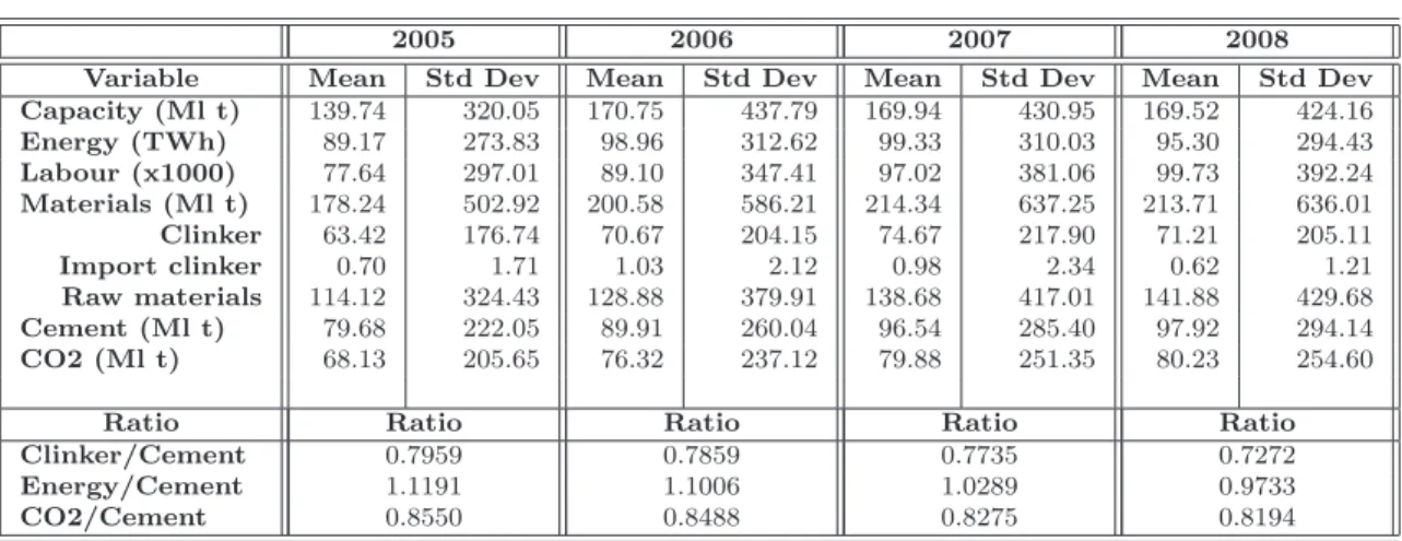
4.3 Database description . . . 66
4.4 Empirical Results . . . 68
4.4.1 Eco-efficiency measure as input and pollutant contraction . . . 69
4.4.2 Eco-efficiency measure as pollutant contraction . . . 72
4.4.3 Eco-efficiency as input contraction . . . 73
4.4.4 Eco-efficiency as undesirable output contraction and desirable output expansion 75 4.5 Conclusions . . . 77
5 Evaluating the efficiency of the cement 79 5.1 Introduction . . . 79
5.2 Model specification . . . 80
5.2.1 A first model comparison: standard BCC DEA model and undesirable factors treated as inputs . . . 81
5.2.2 A second model comparison: the directional distance function approach and undesirable factors treated as output . . . 83
5.2.3 Construction of the production frontier . . . 84
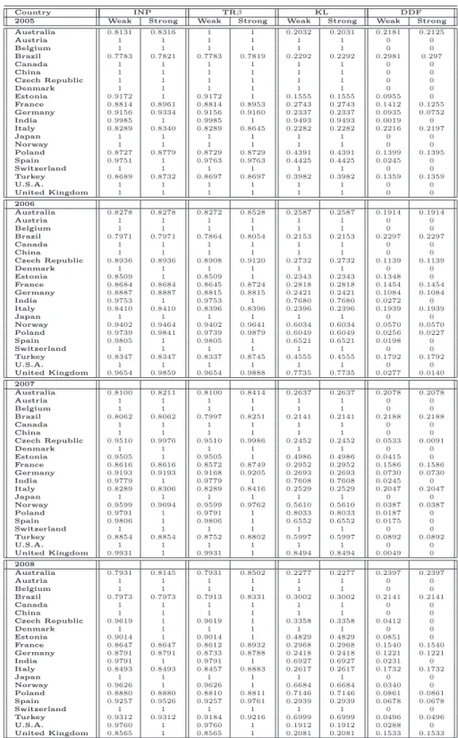
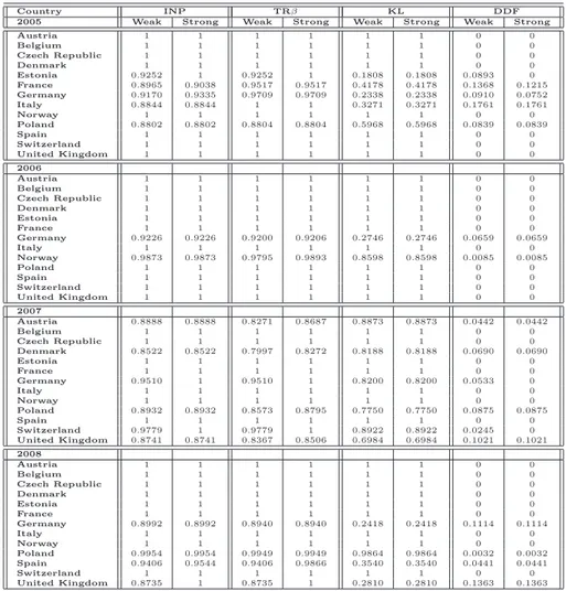
5.3 Empirical Results . . . 85
5.3.1 Efficiency evaluation: standard BCC DEA model and undesirable factors treated as inputs . . . 86
5.3.2 Efficiency evaluation: the directional distance function approach and undesir-able factors treated as output . . . 92
5.3.3 Overall comments . . . 98
5.4 Conclusions . . . 99
6 Conclusions 101 A Simulations 105 A.1 Cement: first instance . . . 106
A.1.1 Contemporaneous frontier for representative plants: European and non-European countries . . . 107
A.1.2 Contemporaneous frontier with aggregated data: European and non-European countries . . . 108
A.1.3 Sequential frontier for representative plants: European and non-European countries . . . 109
A.1.4 Sequential frontier with aggregated data: European and non-European countries110 A.2 Cement: second instance . . . 111
A.2.1 Contemporaneous frontier for representative plants: European and non-European countries . . . 112
A.2.2 Contemporaneous frontier with aggregated data: European and non-European countries . . . 113
A.2.3 Sequential frontier for representative plants: European and non-European countries . . . 114
A.2.4 Sequential frontier with aggregated data: European and non-European countries115 A.3 Cement: third instance . . . 116
A.3.1 Contemporaneous frontier for representative plants: European and non-European countries . . . 117
A.3.2 Contemporaneosu frontier with aggregated data: European and non-European countries . . . 118
A.3.3 Sequential frontier for representative plants: European and non-European countries . . . 119
CONTENTS iii
A.3.4 Sequential frontier with aggregated data: European and non-European countries120
A.4 Clinker instance . . . 121
A.4.1 Contemporeneous frontier for representative plants: European and non-European countries . . . 122
A.4.2 Contemporaneous frontier for representative plants: European countries . . . 123
A.4.3 Contemporaneous frontier with aggregated data: European and non-European countries . . . 124
A.4.4 Contemporaneous frontier with aggregated data: European countries . . . 125
A.4.5 Sequential frontier for representative plants: European and non-European countries . . . 126
A.4.6 Sequential frontier for representative plants: European countries . . . 127
A.4.7 Sequential frontier with aggregated data: European and non-European countries128
A.4.8 Sequential frontier with aggregated data: European countries . . . 129
A.5 Cement without undesirable factor: first instance . . . 130
A.5.1 Contemporaneous frontier for representative plants: European and non-European countries . . . 130
A.5.2 Contemporaneous frontier with aggregated data: European and non-European countries . . . 130
A.5.3 Sequential frontier for representative plants: European and non-European countries . . . 131
A.5.4 Sequential frontier with aggregated data: European and non-European countries131
A.6 Cement without undesirable factor: second instance . . . 132
A.6.1 Contemporaneous frontier for representative plants: European and non-European countries . . . 132
A.6.2 Contemporaneous frontier with aggregated data: European and non-European countries . . . 132
A.6.3 Sequential frontier for representative plants: European and non-European countries . . . 133
A.6.4 Sequential frontier with aggregated data: European and non-European countries133
A.7 Cement without undesirable factor: third instance . . . 134
A.7.1 Contemporaneous frontier for representative plants: European and non-European countries . . . 134
A.7.2 Contemporaneous frontier with aggregated data: European and non-European countries . . . 134
A.7.3 Sequential frontier for representative plants: European and non-European countries . . . 135
A.7.4 Contemporaneous frontier with aggregated data: European and non-European countries . . . 135
A.8 Clinker without undesirable factor instance . . . 136
A.8.1 Contemporaneous frontier for representative plants: European and non-European countries . . . 136
A.8.2 Contemporaneous frontier for representative plants: European countries . . . 136
A.8.3 Contemporaneous frontier with aggregated data: European and non-European countries . . . 137
A.8.4 Contemporaneous frontier with aggregated data: European countries . . . 137
A.8.5 Sequential frontier for representative plants: European and non-European countries . . . 138
A.8.6 Sequential frontier for representative plants: European countries . . . 138
A.8.7 Sequential frontier with aggregated data: European and non-European countries139
iv CONTENTS
B Database Sources 141
Chapter 1
Introduction
Data Envelopment Analysis (DEA) is a data-oriented approach for performance evaluation and improvement of a set of peer entities called Decision Making Units (DMUs) which convert multiple inputs into multiple outputs. The definition of a DMU is generic and flexible. The interest in DEA techniques and their applications is highly increased in the recent literature. In this light, basic DEA models and techniques have been well documented in [16, 19, 20, 48]. Literature shows a great variety of applications of DEA in evaluating performances of entities in different countries (see [17, 23, 66] for an extensive survey of DEA research covering theoretical developments as well as ”real-world” applications). One reason is that DEA can be used for use in cases which have been resistant to other approaches because of the complex (often unknown) nature of the relations the multiple inputs and multiple outputs involved (e.g. in the case of non-commeasurable units).
Starting from the pioneering papers by Charnes, Cooper and Rhodes (CCR model) and Banker, Charnes and Cooper (BCC model) (see [5, 14]) and their originals formulation of data envelopment analysis, in this Ph.D thesis alternative DEA model which consider uncertain and undesirable outputs are taken into account. Classical models assume a deterministic framework with no uncertainty and this seems unsuitable for concrete applications, due to the presence of errors and noise in the estimation of inputs and outputs values. For this reason, the first goal of this work is to propose, starting from the generalized input-oriented (BCC) model, two different models with uncertain outputs and deterministic inputs. Various applications, in fact, are affected by random perturbations in output values estimation (see, for instance, [9, 56, 58]). Random perturbations can be motivated by a concrete difficulty in estimating the right output value (for instance, in the case of energy companies, electricity production has to take care of different and uncertain energy dispersion factors according to the employed technologies) or to obtain good output provisions (for instance, in the case of DEA applied to health care problems, early screening efficiency measures are related to the estimation of true positive and false positive screens which are indeed outputs with a stochastic nature). In particular, two different models are proposed where uncertainty is managed with a scenario generation approach. For the sake of completeness, these models are compared with two further ones based on an expected value approach, that is to say that the uncertainty is managed by means of the expected values of random factors both in the objective function and in the constraints. Deeply speaking, the main difference between the two proposed models and the expected value approaches lies in their mathematical formulation. In the models based on the scenario generation approach, the constraints concerning efficiency level are expressed for each scenario, while in the expected value models they are satisfied in expected value. As a consequence, the first kind of models result to be more selective in finding a ranking of efficiency, thus becoming useful strategic management tools aimed to determine a restrictive efficiency score ranking. The main research results are collected in [50], accepted for publication in the Journal of Information &
2 CHAPTER 1. INTRODUCTION
Optimization Sciences.
In a second part of this study, we focus on the environmental policy and the concept of eco-efficiency. One of the most intensively discussed concepts in the international political debate today is, in fact, the concept of sustainability and the need for eco-efficient solutions that enable the production of goods and services with less energy and resources and with less waste and emissions. In particular, we consider the environmental impact of CO2in cement and clinker production
pro-cesses. Cement industry is, in fact, responsible for approximately 5% of the current worldwide CO2
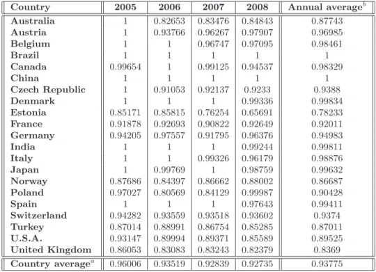
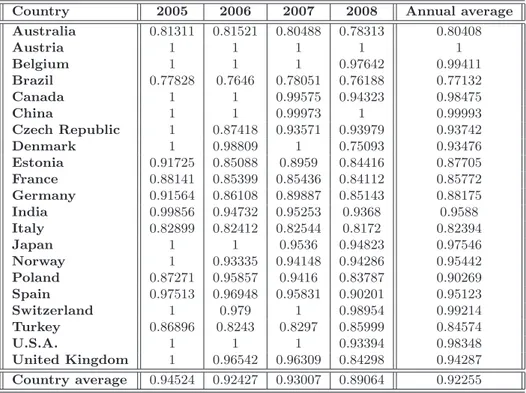
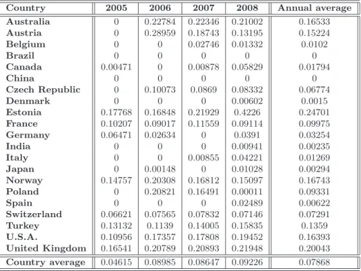
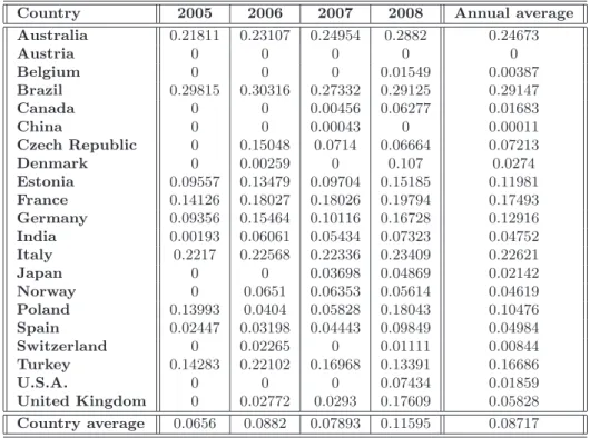
emissions. DEA models can provide an appropriate methodological approach for developing eco-efficiency indicators. With eco-eco-efficiency, we indicate the possibility of producing goods (or services) by reducing the quantity of energy and resources employed and/or the amount of waste and emissions generated. We provide different eco-efficiency measures by applying variants of DEA approaches, where emissions can be either considered as inputs or undesirable outputs. The standard DEA mod-els, in fact, rely on the assumption that inputs are minimized and outputs are maximized. However, when some outputs are undesirable factors (e.g., pollutants or wastes), these outputs should be re-duced to improve efficiency. For this reason, in DEA approach, emissions can be considered either as inputs or as undesirable outputs. This leads to different eco-efficiency measures. In the first part of the analysis, we provide an eco-efficiency measure for 21 prototypes of cement industries operating in many countries by applying both a data envelopment analysis and a directional distance function approach, which are particularly suitable for models where several production inputs and desirable and undesirable outputs are taken into account. Several studies have been carried out to monitor CO2 emission performance trends in different countries and sectors (see, for instance, [57, 64, 66]).
However, to the best of our knowledge, few papers treat undesirable outputs of cement sector as a DEA model and in all of them only interstate analyzes have been developed (Bandyopadhyay [3], Mandal and Madheswaran [40] and Sadjadi and Atefeh [54]). This work differs from previous literature because it compares 21 countries covering 90% of the world’s cement production. To understand whether this eco-efficiency is due to a rational utilization of inputs or to a real carbon dioxide reduction as a consequence of environmental regulation, we analyze the cases where CO2
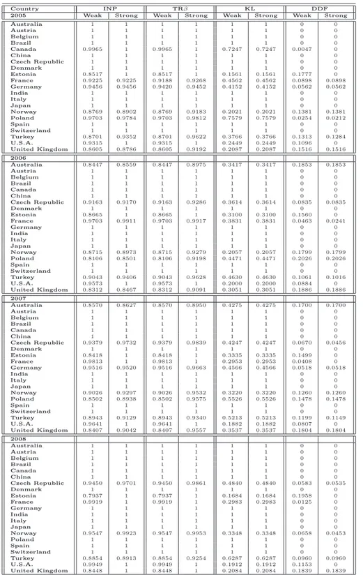
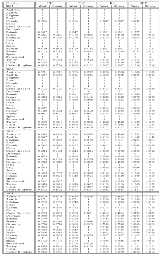
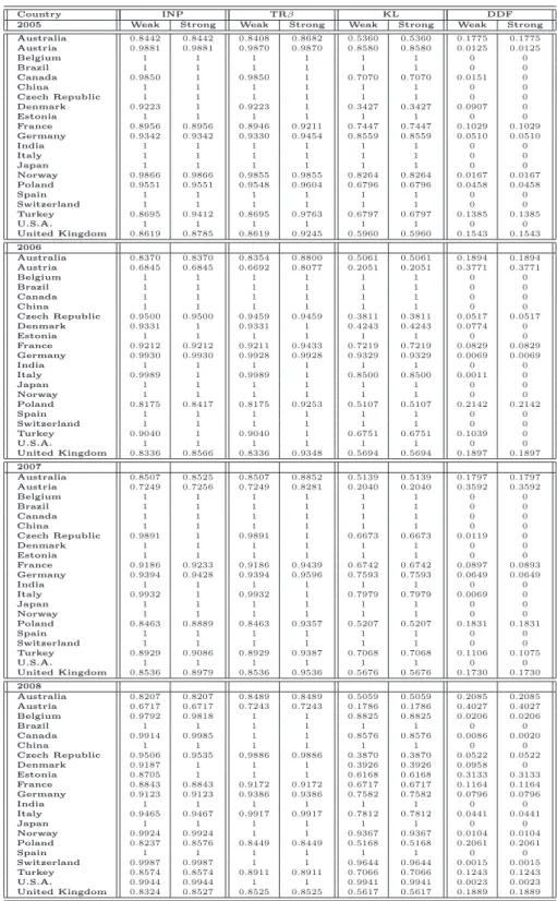
emissions can either be considered as an input or as an undesirable output. The obtained results are collected in [51], accepted for publication in journal Energy Policy. In the second part of the eco-efficiency analysis, we try to answer to the following questions: do undesirable factors modify the efficiency levels of cement industry? Is it reasonable to omit CO2emissions in evaluating the
perfor-mances of the cement sector in different countries? In order to answer to these questions, alternative formulations of standard Data Envelopment Analysis model and directional distance function are compared both in presence and in absence of undesirable factors. The obtained results are collected in [53] and submitted to journal Resource and Energy Economics. Above mentioned studies have been developed taking into account a specific assumption, namely that the production possibility set can be expanded each year, and no technological regress is admitted. In the formulation of DEA models, this assumption can be incorporated through the construction of so-called sequential frontier. Results on eco-efficiency measure through the standard Contemporaneous Frontier, where the frontier in each year is constructed with only the observations of the year under consideration, are collected in [52].
The thesis is divided into the following chapters. Chapter 2 contains a survey of data en-velopment analysis literature. In Chapter 3 two new models for Data Enen-velopment Analysis with uncertain outputs are proposed, with the aim to manage uncertainty through a scenario generation approach. Chapters 4 and 5 focus on the study of DEA models, extending the study of efficiency in case of undesirable factors arising from the production process. In particular, Chapter 4 provide an eco-efficiency measure for twenty-one prototypes of cement industries operating in many countries by applying both a Data Envelopment Analysis and a directional distance function approach, which are particularly suitable for models where several production inputs and desirable and undesirable outputs are taken into account. In Chapter 5 alternative formulations of standard Data Envelopment
3
Analysis model and directional distance function are compared both in presence and in absence of undesirable factors to understand if undesirable factors can modify the efficiency levels of cement in-dustry. Finally, for the sake of completeness, two appendixes are provided. Appendix A contains the tables collecting all of the results of the deep preliminary tests that lead to obtain the ones exposed in Chapter 4 and 5. Finally, in Appendix B the main web sources for our database construction are collected. The original results of this Ph.D. thesis have been collected in the following research papers:
• Riccardi R. and R. Toninelli. Data Envelopment Analysis with outputs uncertainty. Journal of Information & Optimization Sciences, to appear.
• Riccardi R., Oggioni G. and R. Toninelli. The cement industry: eco-efficiency country
compar-ison using Data Envelopment Analysis. Journal of Statistics & Management Systems, accepted
for publication.
• Riccardi R., Oggioni G. and R. Toninelli. Eco-efficiency of the world cement industry: A Data
Envelopment Analysis. Energy Policy, Vol. 39, Issue 5, p. 2842-2854, 2011, available online
at: http://dx.doi.org/10.1016/j.enpol.2011.02.057
• Riccardi R., Oggioni G. and R. Toninelli. Evaluating the efficiency of the cement sector in
presence of undesirable output: a world based Data Envelopment Analysis. Technical Report n.
344, Department of Statistics and Applied Mathematics, University of Pisa, 2011, submitted to Resource and Energy Economics.
The research topic considered in this thesis shows many different lines for future developments. In particular, from a theoretical point of view, starting from the models proposed in [50] we are studying for a bi-objective like DEA formulation where both uncertainty desirable and undesirable factor are taken into account. As regards the applicative aspects, we are also studying and applying bootstrap techniques to manage uncertainty and generate empirical distributions of efficiency scores, in order to capture and analyze the sensitivity of samples with respect to changes in the estimated frontier.
Chapter 2
Data Envelopment Analysis: an
overview
This chapter contains a brief and absolutely not exhaustive survey of data envelopment analysis, in particular of DEA with uncertainty and undesirable data. Some known properties of data en-velopment analysis, especially the ones more related to this Ph.D. thesis, are recalled. An outline of the more recent developments in the field will be also given. This chapter is primarily based on [16, 19, 20, 48], which are among the most popular books on data envelopment analysis. Some of the results recalled in this chapter are given without the proof, please refer to the corresponding bibliographic source for the complete theorem. In section 2.1 the classic DEA models are presented. The section 2.2 takes in account uncertainty data and describes some of the most popular chance-constrained models. In section 2.3 the main DEA models with undesirable outputs are provided.
2.1
DEA models
Data Envelopment Analysis (DEA) is a data oriented approach method for evaluating the perfor-mance of a set of entities called Decision Making Units (DMUs) which convert multiple inputs into multiple outputs. The definition of a DMU is generic and flexible. Recent years have seen a great variety of applications of DEA for use in evaluating the performances of many different kinds of entities engaged in many different activities in many different contexts in many different countries. DEA applications have used DMUs of various forms to evaluate the performance of entities, such as hospitals, universities, cities, courts, business firms, and others, including the performance of coun-tries, regions, etc. Because it requires very few assumptions, DEA has also opened up possibilities for use in cases which have been resistant to other approaches because of the complex (often un-known) nature of the relations between the multiple inputs and multiple outputs involved in DMUs. DEA’s empirical orientation and the absence of a need for the numerous a priori assumptions that accompany other approaches (such as standard forms of statistical regression analysis) have resulted in its use in a number of studies involving efficient frontier estimation in the governmental and non-profit sector, in the regulated sector, and in the private sector. These kinds of applications extend to evaluating the performances of cities, regions and countries with many different kinds of inputs and outputs that include ”social” and ”safety-net” expenditures as inputs and various ”quality-of-life” dimensions as outputs. See [17, 23, 66] for an extensive survey of DEA research covering theoretical developments as well as ”real-world” applications.
In their originating study, Charnes, Cooper and Rhodes [14] described DEA as a ’mathe-matical programming model applied to observational data [that] provides a new way of obtaining
6 CHAPTER 2. DATA ENVELOPMENT ANALYSIS: AN OVERVIEW
empirical estimates of relations - such as the production functions and/or efficient production possi-bility surfaces - that are cornerstones of modern economies’. In fact, DEA proves particularly adept at uncovering relationships that remain hidden from other methodologies. For instance, consider what one wants to mean by ”efficiency”, or more generally, what one wants to mean by saying that one DMU is more efficient than another DMU. This is accomplished in a straightforward manner by DEA without requiring explicitly formulated assumptions and variations with various types of models such as in linear and nonlinear regression models.
We assume that there are n DMUs to be evaluated. Each DMU consumes varying amounts of m different inputs to produce q different outputs. Specifically, DMU j consumes amount xij of
input i and produces amount yrj of output r. We assume that xij ≥ 0, i = 1, . . . , m, j = 1, . . . , n
and yrj≥ 0, r = 1, . . . , q, j = 1, . . . , n and further assume that each DMU has at least one positive
input and one positive output value.
2.1.1
CCR DEA Model
A fractional programming model known as the CCR model was developed by Charnes, Cooper and Rhodes [14] to determine the efficiency score of each of the DMUs in a data set of comparable units. In this form, the ratio of outputs to inputs is used to measure the relative efficiency of the DMU
j0 to be evaluated relative to the ratios of all of DMU j, j = 1, 2, ..., n. We can interpret the CCR
construction as the reduction of the multiple-output/multiple-input situation (for each DMU) to that of a single ’virtual’ output and ’virtual’ input, through the choice of appropriate multipliers, as weighted sum of inputs and weighted sum of outputs. For a particular DMU the ratio of this single virtual output to single virtual input provides a measure of efficiency that is a function of the multipliers. The weights are chosen in a manner that assigns a best set of weights to each DMU. The term ”best” is used here to mean that the resulting input to output ratio for each DMU is maximized relative to all other DMU when these weights are assigned to these inputs and outputs for every DMU. The objective function maximizes the efficiency of the DMU using the weights µr
and νi for each outputs r and each inputs i respectively. The mathematical formulation is provided
below. max µ,ν q X r=1 µryrj0 m X i=1 νixij0 , (2.1)
where it should be noted that the variables are the µ = (µ1, . . . , µr, . . . , µq) and the ν = (ν1, . . . , νi, . . . , νm)
and the yj0 = (y1j0, . . . , yrj0, . . . , yqj0) and xj0 = (x1j0, . . . , xij0, . . . ,
xmj0) are the observed output and input values, respectively, of DMU j0, the DMU to be evaluated. Of course, without further additional constraints (developed below) problem (2.1) is unbounded. A set of normalizing constraints (one for each DMU) reflects the condition that the virtual output to virtual input ratio of every DMU, including DMU j0, must be less than or equal to unity. The
2.1. DEA MODELS 7
mathematical programming problem may thus be stated as ( fPC) max µ,ν z = q X r=1 µryrj0 m X i=1 νixij0 (2.2) s.t. q X r=1 µryrj m X i=1 νixij ≤ 1, j = 1, . . . , n, (2.3) µr≥ 0, r = 1, . . . , q, νi≥ 0, i = 1, . . . , m,
where µr ≥ 0, r = 1, . . . , q, and νi ≥ 0, i = 1, . . . , m have at least one positive value. The
above ratio form yields an infinite number of solutions; if (µ∗, ν∗) is an optimal solution of ( fP C),
then (αµ∗, αν∗) is also optimal for α > 0. However, this fractional problem can be converted into
a linear program through the transformation developed by Charnes and Cooper [13] selecting a representative solution [i.e., the solution (µ, ν) for which
m
X
i=1
νixij0 = 1]. The equivalent linear programming problem in which the change of variables from (µr, νi) to (ur, vi) is a result of the
Charnes-Cooper transformation, (PC) max u,v z = q X r=1 uryrj0 (2.4) s.t. m X i=1 vixij0= 1, (2.5) q X r=1 uryrj− m X i=1 vixij≤ 0, j = 1, . . . , n, (2.6) ur≥ 0, r = 1, . . . , q, (2.7) vi≥ 0, i = 1, . . . , m. (2.8)
This primal formulation, whose objective is to maximize outputs while using at least the give inputs levels, resulting to imposing the condition that Pmi=1νixij0 = 1, is known as input-oriented CCR. There is another type of model that attempts to minimize inputs while using no more than the observed amount of outputs. This is referred to as the output-oriented model.
Theorem 2.1.1 The fractional program (PC) is equivalent to ( fPC).
Proof Under the nonzero assumption of viand xij, the denominator of the constraint (2.3) is positive
8 CHAPTER 2. DATA ENVELOPMENT ANALYSIS: AN OVERVIEW
note that a fractional number is invariant under multiplication of both numerator and denominator by the same nonzero number. After making this multiplication, we set the denominator of (2.2) equal to 1, move it to a constraint, as is done in (2.5), and maximize the numerator, resulting in (PC). Let an optimal solution of (PC) be (v∗, u∗) and the optimal objective value z∗. The solution
(µ∗, ν∗) is also optimal for ( fP
C), since the above transformation is reversible under the assumptions
above. ( fPC) and (PC) therefore have the same optimal objective value z∗.
We also note that the measures of efficiency we have presented are ”units invariant” i.e., they are independent of the units of measurement used in the sense that multiplication of each input by a constant ti > 0, i = 1, . . . , m and each output by a constant pr> 0, r = 1, . . . , q does not change
the obtained solution. Stated in precise form we have
Theorem 2.1.2 (Units Invariance Theorem) The optimal values of max z = z∗ in (P C) and
( fPC) are independent of the units in which the inputs and outputs are measured provided these units
are the same for every DMU.
Proof Let (z∗, u∗, v∗) be optimal for ( fP
C). Now replace the original yrj and xij by pryrj and tixij
for some choices of pr, ti> 0. But then choosing u0= u∗/p and v0= v∗/t we have a solution to the
transformed problem with z0 = z∗. An optimal value for the transformed problem must therefore
have z0 ≥ z∗. Now suppose we could have z0 > z∗. Then, however, u = u0p and v = v0t satisfy
the original constraints so the assumption z0≥ z∗ contradicts the optimality assumed for z∗ under
these constraints. The only remaining possibility is z0 = z∗. This proves the invariance claimed for
(2.2). Theorem 2.1.1 demonstrated the equivalence of (PC) to ( fPC) and thus the same result must
hold and the theorem is therefore proved.
Thus, one person can measure outputs in miles and inputs in gallons of gasoline and quarts of oil while another measures these same outputs and inputs in kilometers and liters. They will nevertheless obtain the same efficiency value from (PC) and ( fPC) when evaluating the same collection
of DMU using different units of measurement.
Let us suppose we have an optimal solution of (PC) for DMU j0 which we represent by
(z∗, u∗, v∗) where u∗ and v∗ are values with constraints given in (2.7) and (2.8). We can then
identify whether CCR-efficiency has been achieved as follows:
Definition 2.1.1 (CCR-Efficiency) For a CCR model,
1. DMU j0 is CCR-efficient if z∗ = 1 and there exists at least one optimal (u∗, v∗), with u∗> 0
and v∗> 0;
2. Otherwise, DMU j0 is CCR-inefficient.
For input-oriented problem (PC), a dual equivalent formulation can be obtained as follows:
(DC) min θ,λ θ s.t. n X j=1 λjyrj≥ yrj0, r = 1, . . . , q, (2.9) n X j=1 λjxij ≤ θxij0, i = 1, . . . , m, (2.10) λj ≥ 0, j = 1, . . . , n,
2.1. DEA MODELS 9
where θ and λ = (λ1, . . . , λj, . . . , λn) are the dual variables corresponding to the primal constraints.
This last model, (DC), is sometimes referred to as the ”Farrell model” because it is the one used
in Farrell [30]. By virtue of the dual theorem of linear programming we have z∗ = θ∗. Hence
either problem may be used. One can solve say (DC), to obtain an efficiency score. Because we
can set θ = 1 and λj0 = 1 and all other λj = 0, j = 1, . . . , n, j 6= j0, a solution of (DC) always exists. Moreover this solution implies θ ≤ 1. The optimal solution, θ yields an efficiency score for a particular DMU j0. The process is repeated for each DMU and DMUs for which θ < 1 are
inefficient, while DMUs for which θ = 1 are boundary points. In the dual input-oriented formulation, the variable θ represents the reduction inputs factor, which states how much the inputs consumed by DMU j0 can be reduced in order to improve its efficiency.
The other type of dual model formulation, that attempts to maximize outputs while using no more than the observed amount of any input, referred to as the output-oriented model, is formulated as: (DCO) max η,τ η s.t. n X j=1 τjyrj ≥ ηyrj0, r = 1, . . . , q, (2.11) n X j=1 τjxij≤ xij0, i = 1, . . . , m. (2.12) τj≥ 0, j = 1, . . . , n.
Theorem 2.1.3 Let (θ∗, λ∗) an optimal solution for the input oriented model (D
C). Then (θ1∗,θ ∗
λ∗) =
(η∗, τ∗) is an optimal solution for the corresponding output oriented (D
CO). Similarly if (η
∗, τ∗) is
optimal for the output oriented model then ( 1
η∗,η ∗
τ∗) = (θ∗, λ∗) is optimal for the input oriented model.
From the above relations, we can conclude that an input-oriented CCR model will be efficient for any DMU if and only if it is also efficient when the output-oriented CCR model is used to evaluate its performance.
The concept of efficiency in production has received a precise meaning when Koopmans and Debreau introduced in 1951 the production set notion, also known as production technology set, in the theory of production. A production technology set is a collection T of pairs (x, y) that have the property of being feasible ones. By feasible it means that the quantities are such that the output y can physically be produced by making use of the input x. In formal terms:
T = {(x, y) : x ∈ R+, y ∈ R+; (x, y) is feasible} .
In DEA we construct a benchmark technology from the observed input-output bundles of the firms in the sample. For this, we make the following general assumptions about the production technology without specifying any functional form. These are fairly weak assumption and holds for all technologies represented by a quasi-concave and weakly monotonic production function:
Assumptions 2.1.1 Properties of the Production Possibility Set T .
Let xj = (x1j, x2j, . . . , xnj) and yj = (y1j, y2j, . . . , yqj) for j = 1, . . . , n the input-output bundle for
10 CHAPTER 2. DATA ENVELOPMENT ANALYSIS: AN OVERVIEW (Al) The input-output bundle (xj, yj) j = 1, . . . , n belong to T.
(A2) The production possibility set is convex. Consider two feasible input-output bundle (xj1, yj1)
and (xj2, yj2). Then, the weighted average input-output bundle (x, y), obtained as x = λxj1+
(1 − λ)xj2 and y = λyj1+ (1 − λ)yj2 for some λ satisfying 0 ≤ λ ≤ 1 is also belong to T .
(A3) Inputs are freely disposable. If (xj0, yj0) j = 1, . . . , n belong to T , then for any x ≥ xj0, (x, yj0)
is also feasible.
(A4) Outputs are freely disposable. If (xj0, yj0) for j = 1, . . . , n belong to T , then for any y ≤ yj0, (xj0, y) is also feasible.
(A5) If, additionally, we assume CRS holds: Let x =Pnj=1xj and y =
Pn
j=1yj. If (x,y) is feasible, then for any k ≥ 0, (kx, ky) if feasible.
Under the hypothesis of constant return to scale, we can define the production possibility set
TC satisfying (Al) through (A5) by
TC= (x, y) : x ≥ n X j=1 λjxj; y ≤ n X j=1 λjyj; λj≥ 0, j = 1, . . . , n . (2.13)
The constraints of (DC) require the bundle (θxj0, yj0) to belong to TC, while the objective seeks the minimum θ that reduces the input vector xj0 radially to θxj0 while remaining in TC. In (DC), we are looking for an activity in TC that guarantees at least the output level yj0 of DMU j0 in all components while reducing the input vector xj0 proportionally (radially) to a value as small as pos-sible. Under the assumptions of the preceding section, it can be said that³Pnj=1λjxj,
Pn
j=1λjyj
´ outperforms (θxj0, yj0) when θ
∗ < 1. With regard to this property, we define the input excesses
s−= (s−
1, . . . , s−i , . . . , s−m) and the output shortfalls s+= (s+1, . . . , s+r, . . . , s+q) and identify them as
”slack” vectors by:
s− = θxj0− n X j=1 λjxj, s+= n X j=1 λjyj− yj0, (2.14)
with s−≥ 0, s+≥ 0 for any feasible solution (θ, λ) of (D
C).
Under this consideration, problem (DC) can be rewritten as:
(dDC) min θ,λ θ s.t. n X j=1 λjyrj= yrj0+ sr +, r = 1, . . . , q, (2.15) n X j=1 λjxij = θxij0+ si −, i = 1, . . . , m, (2.16) λj≥ 0, j = 1, . . . , n, sr+≥ 0, r = 1, . . . , q, si− ≥ 0, i = 1, . . . , m.
2.1. DEA MODELS 11 Definition 2.1.2 If an optimal solution (θ∗, λ∗, s+∗, s−∗) satisfies θ∗= 1 and is zero-slack (s+∗ =
0, s−∗ = 0), then the DMU j
0 is called efficient. Otherwise, the DMU is called
CCR-inefficient, because i. θ∗= 1;
ii. All slacks are zero;
must both be satisfied if full efficiency is to be attained.
The first of these two conditions is referred to as ”radial efficiency.” It is also referred to as ”technical efficiency” because a value of θ∗< 1 means that all inputs can be simultaneously reduced
without altering the mix (=proportions) in which they are utilized. Because (1 − θ∗) is the maximal
proportionate reduction allowed by the production possibility set, any further reductions associated with nonzero slacks will necessarily change the input proportions. Hence the inefficiency is associated with any nonzero slack variables. When attention is restricted to condition (i) in Definition 2.1.2 the term ”weak efficiency” is sometime used to characterize this inefficiency. The conditions (i) and (ii) taken together describe what is also called ”Pareto-Koopmans” or ”strong” efficiency, which can be verbalized as follows
Definition 2.1.3 (Pareto-Koopmans Efficiency) A DMU is fully efficient if and only if it is not possible to improve any input or output without worsening some other input or output.
We have already given a definition of CCR-efficiency for the model in the primal formulation. We now prove that the CCR-efficiency above, gives the same efficiency characterization as is obtained from Definition 2.1.1. This is formalized by:
Theorem 2.1.4 The CCR-efficiency given in Definition 2.1.2 is equivalent to that given by Defini-tion 2.1.1.
Proof First, notice that the vectors u and v of (PC) are dual multipliers corresponding to the
constraints (2.9) and (2.10) of (DC), respectively. Now the following ”complementary conditions”
hold between any optimal solutions (u∗, v∗) of (P
C) and (λ∗j, s+∗, s−∗) of (dDC).
u∗s+∗= 0 and v∗s−∗= 0. (2.17)
This means that if any component of u∗or v∗is positive then the corresponding component of
s+∗ or s−∗ must be zero, and conversely, with the possibility also allowed in which both components
may be zero simultaneously. Now we demonstrate that Definition 2.1.2 implies Definition 2.1.1.
i. If θ∗ < 1, then DMU j
0 is CCR-inefficient by Definition 2.1.1, since (PC) and (DC) have the
same optimal objective value by virtue of the dual theorem of linear programming.
ii. If θ∗ = 1 and is not zero-slack (s+∗ 6= 0, s−∗ 6= 0), then, by the complementary conditions
above, the elements of u∗or v∗corresponding to the positive slacks must be zero. Thus, DMU
j0is CCR- inefficient by Definition 2.1.1.
iii. Lastly if θ∗ = 1 and zero-slack, then, by the ”strong theorem of complementarity, (P C) is
assured of a positive optimal solution (u∗, v∗) and hence DMU j
0is CCR-efficient by Definition
12 CHAPTER 2. DATA ENVELOPMENT ANALYSIS: AN OVERVIEW
The reverse is also true by the complementary relation and the strong complementarity theorem between (u∗, v∗) and (s+∗, s−∗).
Up to this point, we have been dealing models known as CCR (Charnes, Cooper, Rhodes, [14]) models. If the convexity conditionPnj=1λj= 1 is adjoined, they are known as BCC (Banker,
Charnes, Cooper, [5]) models. This added constraint introduces an additional variable, u0, into
the multiplier problems (PC). As will be seen in the next subsection, this extra variable makes it
possible to effect returns-to-scale evaluations (increasing, constant and decreasing). So the BCC model is also referred to as the VRS (Variable Returns to Scale) model and distinguished form the CCR model which is referred to as the CRS (Constant Returns to Scale) model.
2.1.2
BCC DEA Models
In the literature of classical economics, Returns To Scale (RTS) have typically been defined only for single output situations. RTS are considered to be increasing if a proportional increase in all the inputs results in a more than proportional increase in the single output. Let α represent the proportional input increase and β represent the resulting proportional increase of the single output. Increasing returns to scale prevail if β > α and decreasing returns to scale prevail if β < α. Banker [4], Banker, Charnes and Cooper [5] (BCC model) and Banker and Thrall [6] extend the RTS concept from the single output case to multiple output cases using DEA.
The efficiency of a specific DMU j0 can be evaluated by the BCC model of DEA as follows,
(PV) max u,v,u0 q X r=1 uryrj0+ u0 (2.18) s.t. m X i=1 vixij0= 1, (2.19) q X r=1 uryrj+ u0− m X i=1 vixij ≤ 0, j = 1, . . . , n, (2.20) ur≥ 0, r = 1, . . . , q, vi≥ 0, i = 1, . . . , m.
The dual form of the BCC model represented in (PV) is obtained from the same data which are
then used in the following form, (DV) min θ,λ θ s.t. n X j=1 λjyrj≥ yrj0, r = 1, . . . , q, (2.21) n X j=1 λjxij ≤ θxij0, i = 1, . . . , m, (2.22) n X j=1 λj = 1, (2.23) λj ≥ 0, j = 1, . . . , n.
2.1. DEA MODELS 13
We can define the production possibility set TV for DEA model under the hypothesis of variable
return to scale, taking into account assumptions (Al)-(A4) presented in the previous subsection, by
TV = (x, y) : x ≥ n X j=1 λjxj; y ≤ n X j=1 λjyj; n X j=1 λj = 1 (2.24)
It is clear that a difference between the CCR and BCC models is present in constraintPnj=1λj= 1
in the dual formulation, which is the constraint associated with the free variable u0 in primal
formulation that also does not appear in the CCR model.
As concern problems (PV) and (DV), notice that we confine attention to input-oriented versions of
these efficiency measure models. This specification is necessary because, if under the hypothesis of constant return to scale, input-oriented CCR model will be efficient for any DMU if and only if it is also efficient when the output-oriented CCR model, in the case of variables returns to scale, to a different approach corresponds a different efficiency score.
Analogously to the CCR model, we can rewrite problem (DV) as:
(dDV) min θ,λ θ s.t. n X j=1 λjyrj= yrj0+ sr +, r = 1, . . . , q, (2.25) n X j=1 λjxij = θxij0− si −, i = 1, . . . , m, (2.26) n X j=1 λj= 1, (2.27) λj ≥ 0, j = 1, . . . , n, sr+≥ 0, r = 1, . . . , q, si−≥ 0, i = 1, . . . , m. Let (θ∗
V, λ∗, s−∗, s+∗) an optimal solution for (dDV). Notice that θ∗V is not less than the optimal
objective value θ of (DC) model, since (BCC) imposes one additional constraint,
Pn
j=1λj = 1, so
its feasible region is a subset of feasible region for the CCR model.
It is possible to define efficiency concept under variable returns to scale, as
Definition 2.1.4 (BCC-Efficiency) An optimal solution (θ∗
V, λ∗, s−∗, s+∗) satisfies θV∗ = 1 and has
no slack (s−∗= 0, s+∗= 0), then the DMU j
0is called BCC-efficient, otherwise it is BCC-inefficient.
All the models assume that yrj ≥ 0 and xij ≥ 0, r = 1, . . . , q, i = 1, . . . , m, j = 1, . . . , n.
Also in (PV) all variables are constrained to be non-negative, except for u0 which may be positive,
negative or zero with consequences that make it possible to use optimal values of this variable to identify RTS.
When a DMU j0is efficient with the Definition 2.1.1, the optimal value of u0, i.e. u∗0, in (PV),
can be used to characterize the situation for Returns to Scale.
RTS generally has an unambiguous meaning only if DMU j0is on the efficiency frontier, since
it is only in this state that a tradeoff between inputs and outputs is required to improve one or the other of these elements. However, there is no need to be concerned about the efficiency status in our analyses because efficiency can always be achieved as follows. If a DMU j0is not BCC efficient,
14 CHAPTER 2. DATA ENVELOPMENT ANALYSIS: AN OVERVIEW
we can use optimal values from (DV) to project this DMU onto the BCC efficiency frontier via the
following formulas, ˆ yrj0 = n X j=1 λ∗ jyrj+ s+∗r , r = 1, . . . , q, θˆxij0 = n X j=1 λ∗jxij− s−∗i , i = 1, . . . , m, (2.28) where s+∗
r and s−∗i are the optimum slack variable associeted to the inequality constraints (2.25)
and (2.26) respectively. These are sometimes referred to as the ”CCR Projection Formulas” because Charnes, Cooper and Rhodes (1978) showed that the resulting ˆxij0 ≤ xij0and ˆyrj0 ≥ yrj0 correspond to the coordinates of a point on the efficiency frontier. They are, in fact, coordinates of the point used to evaluate DMU j0 when (DV) is employed.
The following theorem for returns to scale, as obtained from Banker and Thrall [6], identifies RTS with the sign of u∗
0 in (PV) as follows:
Theorem 2.1.5 The following conditions identify the situation for RTS for the BCC model given in (PV).
1. Increasing RTS prevail at (ˆxj0, ˆyj0) if and only if u
∗
0< 0 for all optimal solutions.
2. Decreasing RTS prevail at (ˆxj0, ˆyj0) if and only if u
∗
0> 0 for all optimal solutions.
3. Constant RTS prevail at (ˆxj0, ˆyj0) if and only if u
∗
0= 0 for at least one optimal solution.
Here, it may be noted, (ˆxj0, ˆyj0) are the coordinates of the point on the efficiency frontier which is obtained from (2.28) in the evaluation of DMU j0 via the solution to (dDV). Note, therefore, that a
use of the projection makes it unnecessary to assume that the points to be analyzed are all on the BCC efficient frontier - as was assumed in Banker and Thrall [6].
Now consider again model (DC); this model is the same as the ”envelopment form” of the BBC
model in (DV) except for the fact that the condition
Pn
j=1λj = 1 is omitted. The projection formulas
expressed in (2.28) are the same for both models. We can therefore use these same projections to move all points onto the efficient frontier for (DC) and proceed directly to returns to scale
characterizations for (DC) which are supplied by the following theorem from Banker and Thrall [6].
Theorem 2.1.6 The following conditions identify the situation for RTS for the CCR model given in (DC):
1. Constant returns to scale prevail at (ˆxj0, ˆyj0) if
Pn
j=1λ∗j = 1 in any alternate optimum;
2. Decreasing returns to scale prevail at (ˆxj0, ˆyj0) if
Pn
j=1λ∗j > 1 for all alternate optima;
3. Increasing returns to scale prevail at (ˆxj0, ˆyj0) if Pn
j=1λ∗j < 1 for all alternate optima.
For BBC model it is possible establish (see Ali and Seiford [1]) that the solution of the above linear programming problem with translated data is exactly the same as the solution of the linear programming problem with the original data. Let yrj= yrj+βr, r = 1, . . . , q and xij = xij+zi, i =
1, . . . , m, where β and z are proper translation vectors; without loss of generality it is assumed that
βr > 0, r = 1, . . . , q and zi > 0, i = 1, . . . , m. Based upon the above linear transformation, the
2.1. DEA MODELS 15 (gDV) min θ,λ θ s.t. n X j=1 λjyrj≥ yrj0, r = 1, . . . , q, (2.29) n X j=1 λjxij≤ θxij0, i = 1, . . . , m, (2.30) n X j=1 λj= 1, (2.31) λj≥ 0, j = 1, . . . , n.
Theorem 2.1.7 (Translation Invariance Theorem) For the BBC model: 1. DMU j0 is efficient in (DV) iff DMU j0 is efficient for (gDV);
2. DMU j0 is inefficient in (DV) iff DMU j0 is inefficient for (gDV).
Proof
1. When θ∗ = 1, since Pn
j=1λj = 1 and yrj = yrj + βr, r = 1, . . . , q and xij = xij +
zi, i = 1, . . . , m, constrains (2.29) and (2.30) become
Pn
j=1λjyrj ≥ yrj0 r = 1, . . . , q and Pn
j=1λjxij≤ θxij0 i = 1, . . . , m and so, problem (DV) and problem (gDV) are equivalent.
16 CHAPTER 2. DATA ENVELOPMENT ANALYSIS: AN OVERVIEW
2.2
Chance-constrained DEA models
Data envelopment analysis (DEA) is a technique for estimating the efficiency of production decisions made in private industry or in the not-for-profit sector. Observations located at the production frontier are assigned an efficiency value equal to unity; those behind the frontier are assigned a value less than unity. In other words, production efficiency is no longer taken for granted as a matter of assumption but is determined and tested empirically. As the literature of data envelopment analysis has grown many researchers have felt the need to incorporate stochastic considerations into the model to accommodate the presence of measurement and specification errors. Production relationships are often stochastic in nature. In agriculture the unpredictability of weather makes the input-output relationship stochastic. In manufacturing there may be considerable variability in the quality of output obtained, as attested by the need for statistical quality control. In product development there is uncertainty whether new designs will be technically viable and about the prospective market.
Chance-constrained programming is the most used technique to include noise variations in data and to solve data envelopment analysis problems with uncertainty in data. This kind of approach makes it possible to replace deterministic characterizations in DEA, such as ”efficient” and ”not efficient,” with characterizations such as ”probably efficient” and ”probably not efficient.” Indeed, it is possible to go still further into characterizations such as ”sufficiently efficient,” with associated probabilities of not being correct in making inferences about the performance of a DMU. Recent contributions to this approach are due to Land et al. [36], Olesen [44], Sueyoshi [56], Talluri et al. [58], stating a deterministic equivalent formulation in the case of normally distributed data.
The purpose of this section, however, is to provide a systematic presentation of major devel-opments of chance constrained DEA models that have appeared in the literature. Our analysis will been restricted to what is referred to as the ”E-model”, so named because its objective is stated in terms of optimizing ”expected values”. Most of the other DEA literature on this topic has uti-lized the ”P-model” of chance constrained programming to obtain the ”most probable” occurrences, where also the objective function is represented as a probabilistically condition.
2.2.1
Stochastic dominance
In this subsection, we present basic concepts of efficiency and efficiency dominance, first in deter-ministic contest and after in stochastic one. Consider, for example, variable return to scale and so, BCC model. As we have stressed in Section 2.1.2, we can define the production possibility set TV
by TV = (x, y) : x ≥ n X j=1 λjxj; y ≤ n X j=1 λjyj; n X j=1 λj= 1 . In this case we can able to formulate the following definition:
Definition 2.2.1 (General efficiency dominance) Let (x0, y0) ∈ T
V and (x”, y”) ∈ TV . We
say that (x0, y0) dominates (x”, y”) with respect to the production possibility set T
V if and only if
x0 < x” and y0> y” with strict inequality holding for at least one of the components in the input or
the output vector.
Thus, a point in TV is not dominated if and only if there is no other point in TV which satisfies the
definition. This leads to the following definition of efficiency:
Definition 2.2.2 (Efficiency) DMU j0 is efficient with respect to TV if and only if there is no
2.2. CHANCE-CONSTRAINED DEA MODELS 17
In other word,
Definition 2.2.3 (Efficiency 2) DMU j0 is efficient if it is impossible to find a feasible solution
for the following problem:
n X j=1 λjyrj≥ yrj0, r = 1, . . . , q, n X j=1 λjxij ≤ xij0, i = 1, . . . , m, with λj ≥ 0 j = 1, . . . , n satisfying Pn j=1λj = 1
In order to define stochastic efficiency concept, the following parameters are introduced:.
yrj(ξ) ∈ R+: rthoutput quantity produced by the jthDMU
depending on the random factor ξ,
r = 1, . . . , q, j = 1, . . . , n;
xij(ξ) ∈ R+: ithinput quantity used by the jth DMU
depending on the random factor ξ,
i = 1, . . . , m, j = 1, . . . , n.
The concept of dominance can be extended to stochastic efficiency dominance by jointly comparing the outputs and inputs of the DMU under investigation,with every other observed DMU. Informally, it possible to say that DMU j0 is stochastically not dominated in its efficiency if it is
stochastically impossible to find a feasible alternative which is no worse in all criteria and better for at least one criterion. Since the above definition of stochastic efficiency dominance is very strong, Huang and Li [31] suggested to modify the definition as follows. For a given scalar a α ∈ [0, 1], DMU j0is not stochastically dominated in its efficiency if and only if there is a joint probability less
than or equal to a that some other observed DMU displays efficiency dominance relative to DMU
j0. It can be report the exact mathematical characterizations to this concept of stochastic efficiency
dominance in the following definition (see [9]).
Definition 2.2.4 (α-stochastic efficiency) DMU j0is α-stochastic efficient if and only if for any
λj≥ 0 satisfying Pn j=1λj= 1 we have P n X j=1 λjyrj(ξ) ≥ yrj0(ξ), r = 1, . . . , q, n X j=1 λjxij(ξ) ≤ xij0(ξ), i = 1, . . . , m. ≥ (1 − α),
where ”P” means ”probability”, so they restrict definition of efficiency to the probability of the existence of dominating DMU to be less than α.
2.2.2
LLT model
Land, Lovell and Thore [36] modified the standard DEA model to measure technical efficiency in the presence of random variation in the output produced from a give input bundle. Their chance-constrained DEA model (LLT model) builds on the method of chance-chance-constrained programming
18 CHAPTER 2. DATA ENVELOPMENT ANALYSIS: AN OVERVIEW
(CCP) developed by Charnes and Cooper [13]. The essence of a CCP model is that it allows a positive (although low) probability that one or more inequality restrictions will be violated at the optimal solution of the problem. They developed a chance constrained model in which inputs are assumed to be deterministic and outputs are jointly normal distributed. In this setting,the efficient frontier is a soft margin which may be crossed by a few DMUs. Extending the concept of efficiency in a chance constrained setting the authors stated the equivalence between chance constrained efficiency and Pareto Koopmans efficiency.
The Land, Lovell and Thore chance-constrained input-oriented BCC DEA model can be specified as follows: min θ,λ θ s.t. P Xn j=1 λjyrj(ξ) ≥ yrj0(ξ) ≥ (1 − α), r = 1, . . . , q, (2.32) n X j=1 λjxij≤ θxij0, i = 1, . . . , m, (2.33) n X j=1 λj= 1, (2.34) λj≥ 0, j = 1, . . . , n.
The meaning of the chance constraints is that all the constraints should not be violated with prob-ability at most α. If we assume also random distribution for outputs, we obtain the follows model:
min θ,λ θ s.t. P n X j=1 λjyrj(ξ) ≥ yrj0(ξ) ≥ (1 − α), r = 1, . . . , q, (2.35) P Xn j=1 λjxij(ξ) ≤ θxij0(ξ) ≥ (1 − α), i = 1, . . . , m, (2.36) n X j=1 λj= 1, (2.37) λj ≥ 0, j = 1, . . . , n.
Definition 2.2.5 (Chance Constrained Efficiency) DMU j0 is stochastic efficient if and only
if the following two conditions are both satisfied: i. θ∗= 1;
ii. Slack values are all zero for all optimal solutions.
Although the model has the advantage of making the estimated frontier less sensitive to extreme observations, it introduces a bias due to the normality assumption. Moreover, the proba-bilistic constraints are individually imposed on stochastic inputs/outputs. Thus, the model enables to handle dependencies inter-DMUs, but ignores the correlation intra-DMUs.
2.2. CHANCE-CONSTRAINED DEA MODELS 19
2.2.3
OP model
Olesen and Petersen [45] developed a chance constrained DEA model (OP model) imposing chance constraints on a DEA formulation in multiplier form. They assumed that the inefficiency term of the considered DMU can be decomposed into true inefficiency and disturbance term. In the chance constrained OP model, only observations belonging to confidence region shave to be included in the empirical production possibility set (PPS). Since chance constraints are imposed individually on each DMU, the OP model accounts for correlation among outputs, inputs and inputs/outputs.
max u,v q X r=1 uryrj(ξ) (2.38) s.t. m X i=1 vixij(ξ) = 1, (2.39) P Ã q X r=1 uryrj(ξ) ≤ m X i=1 vixij(ξ) ! ≥ (1 − α), j = 1, . . . , n, (2.40) ur≥ 0, r = 1, . . . , q, vi ≥ 0, i = 1, . . . , m.
2.2.4
Sueyoshi models
Sueyoshi [56] proposed a stochastic DEA model able to incorporate future information. The author referred to this approach as DEA future analysis ˝and applied it to plan the restructure strategy of a Japanese petroleum. In this study is assumed that it can be control the quantity of inputs as the decision variables, whilst being unable to control outputs, because these quantities depend upon external factors such as an economic condition, a demographic change, and other socio-economic factors that influence the magnitude of outputs. Hence, the inputs are considered as deterministic variables and the outputs are considered as stochastic variables. Sueyoshi model, proposed by the author in the primal formulation, is defined as follows:
max u,v Eξ " q X r=1 uryrj0(ξ) # (2.41) s.t. m X i=1 vixij0 = 1, (2.42) P q X r=1 uryrj(ξ) m X i=1 vixij ≤ βj ≥ (1 − αj), j = 1, . . . , n, (2.43) ur≥ 0, r = 1, . . . , q, vi≥ 0, i = 1, . . . , m, where:
20 CHAPTER 2. DATA ENVELOPMENT ANALYSIS: AN OVERVIEW αj∈ [0, 1]: specifies the allowable likehood of falling the jth constraint,
j = 1, . . . , n;
βj∈ [0, 1]: it is refered to as an ”aspiration level”,
specifies the desired efficiency level for the jth
0 DMU,
j = 1, . . . , n.
In other words, the symbol αj stands for a probability that the output/input ratio becomes more
than βj with a choice of weight multipliers. Thus, αj is considered as a risk criterion representing
the utility of a decision maker. On the other hand, 1 − αj indicates the probability of attaining the
requirement. Like βj, the risk criterion (αj) is also a prescribed value that is measured on the range
between 0 and 1. When αj= 0 in constraints (2.43), it is certainly required that the output/input
ratio becomes less than or equal to βj. Conversely, αj = 1 omits the requirement under any selection
of weight multipliers.
It can be easily thought that the above DEA future model needs to be reformulated to obtain its computational feasibility. In particular, through the transformation developed by Charnes and Cooper [13], constraints (2.43) including the stochastic process, can be rewritten as follows:
P à q X r=1 ury˜rj≤ βj à m X i=1 vixij !! ≥ (1 − αj), j = 1, . . . , n, (2.44)
where, for the sake of completeness, the stochastic outputs is expressed as ˜yrj≡ yrj(ξ).
Conditions (2.44) is equivalent to:
P q X r=1 ur(˜yrj− yrj) p Vj ≤ βj m X i=1 vixij− q X r=1 uryrj p Vj ≥ (1 − αj), j = 1, . . . , n, (2.45)
where yrj is the expected value of stochastic outputs ˜yrj and Vj indicates the variance-covariance
matrix of the jth DMU.
These reformulated conditions introduce the following new variable ˜zj:
˜ zj= q X r=1 ur(˜yrj− yrj) p Vj , j = 1, . . . , n, (2.46)
which follows the standard normal distribution with zero mean and unit variance. Substitution of condition (2.46) in constraints (2.45) produces
P z˜j≤ βj m X i=1 vixij− q X r=1 uryrj p Vj ≥ (1 − αj), j = 1, . . . , n. (2.47)
Since ˜zj follows the standard normal distribution, the invertibility of above condition is executed as
2.2. CHANCE-CONSTRAINED DEA MODELS 21 βj m X i=1 vixij− q X r=1 uryrj p Vj ≥ F−1(1 − α j), j = 1, . . . , n. (2.48)
Here, F stands for a cumulative distribution function of the normal distribution and F−1 indicates
its inverse function.
Sueyoshi’s determinist equivalent formulation is then defined as follows: max u,v q X r=1 uryrj0 (2.49) s.t. m X i=1 vixij0 = 1, (2.50) βj m X i=1 vixij− q X r=1 uryrj ≥ p VjF−1(1 − αj), j = 1, . . . , n, (2.51) ur≥ 0, r = 1, . . . , q, vi ≥ 0, i = 1, . . . , m.
Notice that, this kind of resolution method is also applicable to the other chance-constrained model, above mentioned.
2.2.5
Bruni model
The main research field in Stochastic DEA considers a chance-constrained approach which permits constraint violations up to specified probability limits. Bruni et al. [9] introduce a less restrictive formulation than classical chance-constrained approach. The authors take further developments in order to derive a sufficient criterion for efficiency, complementing the Huang and Li approach [32]. They shall assume that the random variables follow a discrete distribution and each realization can be represented by a scenario s. Let us denote by TS the production possibility set for scenario s:
TS= (xs, ys) : n X j=1 λjyrjs ≥ ysrj0, r = 1, . . . , q, s = 1, . . . , S, n X j=1 λjxsij ≤ θxsij0, i = 1, . . . , m, s = 1, . . . , S, n X j=1 λj = 1, λj ≥ 0, j = 1, . . . , n. (2.52)
22 CHAPTER 2. DATA ENVELOPMENT ANALYSIS: AN OVERVIEW impossible to find a feasible solution for the following problem:
n X j=1 λjyrjs ≥ yrjs0, r = 1, . . . , q, (2.53) n X j=1 λjxsij≤ xsij0, i = 1, . . . , m, (2.54) n X j=1 λj = 1, (2.55) λj ≥ 0, j = 1, . . . , n, (2.56)
and strict inequality holding for at least one constraint. Only if for DMU j0 problem (2.53)-(2.56)
is infeasible with respect to the full scenario set, DMU j0 is 100% stochastically efficient.
Bruni et al. propose a model which removes the hypothesis of normal data distribution and uses a scenario generation approach to linearize the problem formulated through the chance-constrained approach. Starting from the LLT model and by adopting a standard technique used in disjunctive programming (see Balas [2]) Bruni et al. defined the deterministic equivalent formulation model for joint probabilistic constraints as:
min θ,λ,δ θ s.t. n X j=1 λjyrjs + Msδs≥ yrjs0, r = 1, . . . , q, s = 1, . . . , S, (2.57) n X j=1 λjxsij≤ θxsij0+ M sδs, i = 1, . . . , m, s = 1, . . . , S, (2.58) S X s=1 psδs≤ (1 − α), (2.59) n X j=1 λj= 1, λj≥ 0, j = 1, . . . , n, δs∈ {0, 1}, s = 1, . . . , S, where: ys
rj ∈ R+: rth output quantity produced by the jthDMU for each
scenario s, r = 1, . . . , q, j = 1, . . . , n, s = 1, . . . , S; xs
ij∈ R+: ith input quantity produced by the jthDMU for each
scenario s, i = 1, . . . , n, j = 1, . . . , n, s = 1, . . . , S; ps∈ [0, 1]: realization probability of any scenario s, s = 1, . . . , S;
δs∈ 0, 1: binary variable for each scenario s, s = 1, . . . , S.
Bruni’s Model, according to chance-constrained approach, permits constraint violations up to a fixed probability level; in particular, constraint (2.59) defines a binary knapsack constraint which guarantees the violation of the stochastic constraints for a subset of scenarios whose cumulative
2.2. CHANCE-CONSTRAINED DEA MODELS 23
probability is less than the complement of the imposed reliability level 1 − α. Stating α = 1 and
ps> 0, the constraint (2.59) forces the binary variables δsto assume the value zero for all scenarios.
This is the situation where it is impossible to violate any constraints so that all the scenarios have to be considered.