A new empirical BESS model for primary control reserve

POLITECNICO DI MILANO

School of Industrial and Information Engineering

Master of Science in Electrical Engineering

A New Empirical BESS Model for Primary Control Reserve

Supervisor: Prof. Marco Merlo

Candidate:

Hamid Malmir

Matr. 877251

Academic Year 2018-2019

II

To my parents Hassan Malmir and Shahrzad Eskandaripour, for giving birth to me in the first place and supporting me spiritually throughout my life, and to my family who always push me forward!

III

Acknowledgement

Foremost, I would like to express my sincere gratitude to my advisor Prof. Marco Merlo for his continuous support, patience, motivation, enthusiasm, and immense knowledge. His guidance helped me in all the time of research and writing of this thesis. I could not have imagined having a better advisor and mentor for my thesis.

Besides my advisor, I would like to thank Dr. Giuliano Rancilio for his friendliness, insightful comments, and continuous helps. I wish him the best luck with his future career.

Last but not the least, I would like to thank my friends, Marzieh Hosseini, Miad Ahmadi, Mahdi Bayat, Salman Oukati, Payam Norouzi, Leila Esfandiari, and Asal Tabaei.

1

Table of content

2 Energy Storage Systems ... 6

2.1 Different Energy Storage Technologies ... 7

2.1.1 Ultracapacitors ... 7

2.1.2 Flywheels ... 8

2.1.3 Fuel cells ... 9

2

2.1.4.1 Primary Batteries ... 11

2.1.4.2 Secondary Batteries ... 11

2.1.4.3 Lithium Batteries ... 12

2.1.4.4 Nickel Cadmium Batteries ... 13

2.1.4.5 Lead Acid Batteries ... 15

2.2 Important parameters of a battery ... 16

2.2.1 Ageing Mechanism and safe operation ... 17

2.2.2 End of life ... 18

2.2.2.1 Cycle life ... 18

2.2.2.2 Warrantied life ... 18

2.2.2.3 Total energy throughput ... 18

2.2.3 Operational life... 18

2.2.4 State of health ... 19

2.2.5 Temperature ... 19

2.2.6 C-rate and E-rate ... 19

2.2.7 Cycles and efficiency ... 20

2.3 Ragone Chart ... 21

2.4 SOC Models ... 22

2.4.1 Coulomb counting ... 23

2.4.2 Voltage-based method ... 23

2.4.3 Physics-based methods ... 24

3

2.4.4.1 Active models ... 27

2.4.4.2 Passive models ... 27

2.4.4.3 Empirical ... 28

3 Ancillary Services Market (ASM) ... 32

3.1 Electricity Market Regulations ... 33

3.1.1 Basic D-ahead market trading principle [80] ... 33

3.2 Ancillary services ... 34

3.2.1 Frequency regulation ... 36

3.2.1.1 Primary Control Reserve (PCR) ... 38

3.2.1.1.1 The BESS Controller ... 40

3.2.1.2 Secondary Control Reserve (SCR) ... 41

3.2.1.3 Tertiary Control Reserve (TCR)... 42

3.2.2 Voltage Control ... 42

3.2.3 System Restoration ... 43

3.3 BESS for Ancillary Services Provision ... 44

4 Methodology ... 48

4.1 Empirical Model for PCR provision ... 49

4.2 PCR controller ... 49

4.3 BESS Empirical model ... 50

4.3.1 BESS model ... 50

4.3.1.1 Overall efficiency ... 51

4

4.3.1.3 SOC update... 54

4.3.1.4 Efficiency computation ... 55

4.4 Validation ... 56

4.4.1 SOC estimation error... 56

4.4.2 Energy estimation error ... 57

4.4.3 Energy flow ... 57

5 Results ... 60

5.1 Validation of the model ... 61

5.1.1 Low initial SOC ... 62

5.1.2 Medium initial SOC ... 63

5.1.3 High initial SOC ... 64

6 Conclusion ... 69

Appendix ... 72

Appendix A: Experimental setup of the BESS ... 72

List of Acronyms ... 75

5

List of Figures

Figure 1.1 Global electricity production in 2050 ... 3

Figure 1.2 Global electricity production by generation type. ... 3

Figure 2.1 Ultracapcitor ... 7

Figure 2.2 Freewheel Layout ... 8

Figure 2.3 Fuel cell structure and stationary application... 9

Figure 2.4 Lithium ion battery structure and Lithium battery cell. ... 12

Figure 2.5 Nickel cadmium battery structure and Nickel cadmium cell. ... 13

Figure 2.6 Lead acid battery structure and Sealed lead acid battery. ... 15

Figure 2.7 Ragone plot ... 21

Figure 2.8 Dual-foil battery electrochemical model ... 25

Figure 2.9 Schematic diagram of the NRC ECM ... 26

Figure 2.10 (a) Active, and (b) Passive ECM... 28

Figure 3.1 Equilibrium point for Day-ahead market ... 34

Figure 3.2 Frequency variation vs. demand power ... 36

6

Figure 3.4 Activation of primary, secondary, and tertiary control after a power imbalance.

... 39

Figure 3.5 Droop control curve for frequency regulation ... 41

Figure 3.7 Number of frequency incidents per month and installed wind power capacity in the Nordic system. ... 45

Figure 4.1 Empirical Model for PCR Provision ... 49

Figure 4.2 BESS model ... 50

Figure 4.3 BESS Model Subblocks ... 51

Figure 4.4 Overall efficiency ... 51

Figure 4.5 The curve of the 𝜂𝐵𝐸𝑆𝑆 ... 52

Figure 4.6 Capability curve block ... 53

Figure 4.7 Capability lookup tables ... 54

Figure 4.8 SOC update ... 55

Figure 4.9 Efficiency computation ... 56

Figure 5.1 Frequency trend, Power setpoint, and SOC estimation with models during PCR ... 62

Figure 5.2 Frequency trend, Power setpoint, and SOC estimation with models during PCR ... 63

Figure 5.3 Frequency trend, Power setpoint, and SOC estimation with models during PCR ... 64

Figure 6.1 BESS scheme with measurement boxes position. ... 72

Figure 6.2 The BESS setup: battery container (a), racks (b), SCADA (c), switchboard and feeder (d). ... 74

7

List of Tables

Table 4.1 BESS efficiency lookup table as implemented in the model ... 52

Table 5.1 Result comparison of the three cases for low SOC ... 65

Table 5.2 Result comparison of the three cases for medium SOC ... 66

Table 5.3 Result comparison of the three cases for high SOC ... 66

Table 5.4 Evaluation of time consumption for electrical and empirical models. ... 67

9

Abstract

Nowadays, with the fast growth of the grid penetration levels of renewable sources, guaranteeing the stability of the grid is becoming more and more difficult than it was in the past. Battery Energy Storage Systems (BESSs) are the most promising solutions for ancillary services provision among which Primary Control Reserve (PCR). Currently, the fastest BESS model is empirical model. Unfortunately, they are not enough accurate in State of Charge (SOC) estimation so that they are only used for the sizing of the battery pack but not the real time SOC monitoring. In this study, the development of an empirical BESS model for SOC estimation based on an experimental data of a Li-ion battery pack is proposed. The aim of this work is to develop a novel empirical model with high accuracy in SOC estimation.

Keywords: Empirical BESS model; battery energy storage system; ancillary services;

10

Sommario

Oggi, con la rapida crescita dei livelli di penetrazione della rete da fonti rinnovabili, garantire la stabilità della rete sta diventando sempre più difficile di quanto non fosse in passato. I sistemi di accumulo dell'energia della batteria (BESSs) sono le soluzioni più promettenti per la fornitura di servizi ausiliari, tra cui la Riserva di controllo primario (PCR). Attualmente, il modello BESS più veloce è il modello empirico. Sfortunatamente, non sono abbastanza precisi nella stima dello stato di carica (SOC) in modo da essere utilizzati solo per il dimensionamento del pacco batteria ma non per il monitoraggio SOC in tempo reale. In questo studio, viene proposto lo sviluppo di un modello empirico BESS per la stima SOC basato su dati sperimentali di un pacco batterie agli ioni di litio. Lo scopo di questo lavoro è di sviluppare un nuovo modello empirico con elevata precisione nella stima SOC.

Parole chiave: modello empirico BESS; sistema di accumulo dell'energia della batteria;

2

Chapter 1

Introduction

The total renewable energy production is doubled by nine years from 2009 to 2018 [1]. As variable renewables grow to substantial levels, electricity systems will require greater flexibility. Unfortunately, most of the Renewable Energy Sources (RESs) are not programmable, so their generated power needs to be stored. Battery energy storage systems (BESSs) are a promising solution for this problem due to their inherent distributed features, their ability to inject and absorb power, their high-power ramping and ability to provide a set of different grid services. As of today, BESSs are being deployed to provide several different services, such as peak shaving [2], energy management of microgrids [3] and stochastic resources [4], [5] and frequency and voltage regulation [6], [7], [8]. By providing these essential services, electricity storage can drive serious electricity decarbonization and help transform the whole energy sector [9]. The Figure 1.1 and Figure 1.2 show Global electricity production in 2050.

3

Figure 1.1 Global electricity production in 2050 [10]

Figure 1.2 Global electricity production by generation type [10].

Recent technology advancement in battery storage in general has been intensified by high demand for batteries in electronic devices. Structural elements indicate not only that continued cost reductions are likely, but also that they are strongly linked to developments underway in the different sectors, for example, changes in battery characteristics (chemistry, energy density and size of the battery packs) and the scale of manufacturing plants. Today most battery production is in plants that range from 3 to 8 gigawatt-hours per year

4

(GWh/year) though three plants with over 20 GWh/year capacity are already in operation and five more are expected by 2023.

It is expected that by 2025 batteries will increasingly use cathode chemistries that are less dependent on cobalt, such as NMC 811,3 NMC 622 or NMC 532 cathodes in the NMC family or advanced NCA batteries. This will cause to an increase in energy density and a decrease of battery costs, in combination with other developments (e.g. the availability of silicon-graphite chemistries for anode technology). In the European Union, the Strategic Action Plan for Batteries in Europe was adopted in May 2018. It brings together a set of measures to support national, regional and industrial efforts to build a battery value chain in Europe, including raw material extraction, sourcing and processing, battery materials, cell production, battery systems, as well as reuse and recycling. In combination with the leverage offered by its market size, it seeks to attract investment and establish Europe as a player in the battery industry [11].

Stationary electricity storage can provide wide variety of energy services in an affordable manner. As the cost of emerging technologies decreases further, storage will become increasingly competitive, and the range of economical services it can provide will increase [9].

The structure of the thesis is outlined in the following. In Chapter 2, an introduction on the different types of energy storage technology and SOC models is given. In chapter 3, Ancillary Services Market is explained. Chapter 4 is about methodology that is used for modeling of the empirical model. The simulations performed with the model presented in Chapter 5 are presented, and in the chapter 6, the conclusion of the model and the simulations results are given.

6

Chapter 2

Energy Storage Systems

The main goal of this chapter is to give a background about energy storage systems, battery parameters, and short review of different battery models. There are several methods to store energy. With advancing the technologies, the number of equipment that can store energy in different ways are increasing. In the following, some of the most popular technology of storing energy is explained.

7

2.1 Different Energy Storage Technologies

2.1.1 Ultracapacitors

Figure 2.1 Ultracapcitor [12]

An ultracapacitor is an electrochemical device consisting of two porous electrodes, usually made up of activated carbon immersed in an electrolyte solution that stores charge electrostatically. This arrangement effectively creates two capacitors, one at each carbon electrode, connected in series. The ultracapacitor is available with capacitances in the hundreds of farads all within a very small physical size and can achieve much higher power density than batteries. However, the voltage rating of an ultracapacitor is usually less than

8

about 3 volts so several capacitors have to be connected in series and parallel combinations to provide any useful voltage.

Ultracapacitors can be used as energy storage devices similar to a battery, and in fact are classed as an ultracapacitor battery. But unlike a battery, they can achieve much higher power densities for a short duration. They are used in many hybrid petrol vehicles and fuel cell driven electric vehicles because of their ability to quickly discharge high voltages and then be recharged. But by operating ultracapacitors with fuel cells and batteries peak power demands, and transient load changes can be controlled more efficiently [12].

2.1.2 Flywheels

Figure 2.2 Freewheel Layout [13], [14]

A flywheel is a mechanical device specifically designed to convert electrical energy to kinetic energy (rotational energy). Flywheels resist changes in rotational speed by their moment of inertia. The amount of energy stored in a flywheel is proportional to the square of its rotational speed and its mass. The way to change a flywheel's stored energy without changing its mass is by increasing or decreasing its rotational speed. Since flywheels act as

9

mechanical energy storage devices, they are the kinetic-energy-storage analogue to electrical inductors, for example, which are a type of accumulator.

Flywheels are typically made of steel and rotate on conventional bearings; these are generally limited to a maximum revolution rate of a few thousand RPM [15]. High energy density flywheels can be made of carbon fiber composites and employ magnetic bearings, enabling them to revolve at speeds up to 60,000 RPM (1 kHz) [16]. Carbon-composite flywheel batteries have recently been manufactured and are proving to be viable in real-world tests on mainstream cars. Additionally, their disposal is more eco-friendly than traditional lithium ion batteries [17].

2.1.3 Fuel cells

Figure 2.3 Fuel cell structure and stationary application [18].

Unlike traditional combustion technologies that burn fuel, fuel cells undergo a chemical process to convert hydrogen-rich fuel into electricity. Fuel cells do not need to be periodically recharged like batteries, but instead continue to produce electricity as long as a fuel source is provided [18].

A fuel cell is composed of an anode, a cathode, and an electrolyte membrane. A fuel cell works by passing hydrogen through the anode of a fuel cell and oxygen through the

10

cathode. At the anode site, the hydrogen molecules are split into electrons and protons. The protons pass through the electrolyte membrane, while the electrons are forced through a circuit, generating an electric current and excess heat. At the cathode, the protons, electrons, and oxygen combine to produce water molecules. Due to their high efficiency, fuel cells are very clean, with their only by-products being electricity, excess heat, and water. In addition, as fuel cells do not have any moving parts, they operate near-silently [18].

Advantages at a glance: • Low-to-Zero Emissions • High Efficiency • Reliability • Fuel Flexibility • Energy Security • Durability • Scalability • Quiet Operation Disadvantages at a glance:

• Average efficiency (lower w.r.t batteries, even lower if you consider the efficiency of the electrolyzer, too)

• low specific power

• Expensive to manufacture due the high cost of catalysts (platinum) • Lack of infrastructure to support the distribution of hydrogen

• A lot of the currently available fuel cell technology is in the prototype stage and not yet validated

11

2.1.4 Batteries

A battery is a device consisting of one or more electrochemical cells with external connections for powering electrical devices [19]. They are classified into two main groups:

2.1.4.1 Primary Batteries

Primary (single-use or "disposable") batteries are used once and discarded, as the electrode materials are irreversibly changed during discharge; a common example is the alkaline battery used for flashlights and a multitude of portable electronic devices [20]. In general, these have higher energy densities than rechargeable batteries [21]. Common types of disposable batteries include zinc–carbon batteries and alkaline batteries.

2.1.4.2 Secondary Batteries

Secondary (rechargeable) batteries can be discharged and recharged multiple times using an applied electric current; the original composition of the electrodes can be restored by reverse current. Examples include the lead-acid batteries used in vehicles and lithium-ion batteries used for portable electronics such as laptops and mobile phones [20].

12

2.1.4.3 Lithium Batteries

Figure 2.4 Lithium ion battery structure [22] and Lithium battery cell [23].

A lithium-ion battery or Li-ion battery (LIB) is a type of rechargeable battery. Lithium-ion batteries are commonly used for portable electronics and electric vehicles and are growing in popularity for military and aerospace applications [24]. The lithium ions within a lithium ion battery migrate back and forth between the two electrodes during charging and discharging. The ions travel between the anode and the cathode via a separator by an electrolyte commonly composed a lithium salt (e.g. LiPF6) in an organic solvent. The electrolyte solution plays a critical role within LIBs by enabling an effective conduction of the lithium ions between the electrodes. Additives are commonly added into the electrolyte solution to improve performance, enhance stability, prevent solution degradation and prevent dendritic lithium formation. The prevention of dendritic lithium formation is key to achieving battery safety as the lithium dendrites establish a connection between the electrodes, causing the battery to overheat and become a potential fire hazard. The electrolytes and their additives are commonly used in LIBs to identify the current density, stability and the reliability of the final battery. The properties of the electrolyte are therefore critical to the overall performance of the battery. Electrolytes must possess a good ionic conductivity and be electrically insulating, they should have a wide electrochemical window, they must be inert to other battery components and they must be chemically and thermally stable. In addition, electrolytes of a high purity (free from contamination) help to prevent oxidation at the electrode and promote a good cycle life [22].

13

This Lithium-ion Battery technology is popular because of the high energy density (high voltage combined with high specific capacity), high discharge rate, and high security and low cost [13].

Advantages at a glance:

• High specific energy and high load capabilities with Power Cells. • Long cycle and extend shelf-life; maintenance-free.

• High capacity, low internal resistance, good coulombic efficiency. • Simple charge algorithm and reasonably short charge times. • Low self-discharge (less than half that of NiCd and NiMH).

Disadvantages at a glance:

• Requires protection circuit to prevent thermal runaway if stressed. • Degrades at high temperature and when stored at high voltage. • No rapid charge possible at freezing temperatures (<0°C, <32°F). • Transportation regulations required when shipping in larger quantities.

2.1.4.4 Nickel Cadmium Batteries

14

Invented by Waldemar Jungner in 1899, the nickel-cadmium battery offered several advantages over lead acid, then the only other rechargeable battery; however, the materials for NiCd were expensive [27]. The nickel cadmium battery consists of a nickel-positive electrode (cathode) and a cadmium-negative electrode (anode) in potassium hydroxide solution [28].

Developments were slow, but in 1932, advancements were made to deposit the active materials inside a porous nickel-plated electrode. Further improvements occurred in 1947 by absorbing the gases generated during charge, which led to the modern sealed NiCd battery. For many years, NiCd was the preferred battery choice for two-way radios, emergency medical equipment, professional video cameras and power tools. In the late 1980s, the ultra-high capacity NiCd rocked the world with capacities that were up to 60 percent ultra-higher than the standard NiCd. Packing more active material into the cell achieved this, but the gain was shadowed by higher internal resistance and reduced cycle count [27].

Advantages at a glance:

• Rugged, high cycle count with proper maintenance.

• Only battery that can be ultra-fast charged with little stress. • Good load performance; forgiving if abused.

• Simple storage and transportation; not subject to regulatory control. • Good low-temperature performance.

• Economically priced; NiCd is the lowest in terms of cost per cycle.

Disadvantages at a glance:

• Relatively low specific energy compared with newer systems.

• Memory effect; needs periodic full discharges and can be rejuvenated. • Cadmium is a toxic metal. Cannot be disposed of in landfills.

• High self-discharge; needs recharging after storage.

15

2.1.4.5 Lead Acid Batteries

Figure 2.6 Lead acid battery structure [29], [30] and Sealed lead acid battery [31].

Invented by the French physician Gaston Planté in 1859, lead acid was the first rechargeable battery for commercial use. Lead acid batteries have been used as energy sources commercially since 1860 [32]. LA batteries are used in every internal combustion engine (ICE) vehicle as a starter and typically applied for uninterrupted power supply (UPS), renewable energy storage, and grid storage because of their ruggedness, safe operation, temperature tolerance, and low cost [33], [30]. The battery consists of Pb as negative electrode, PbO2 as positive electrode, and H2SO4 solution as electrolyte [29], [34]. Despite its advanced age, the lead chemistry continues to be in wide use today. There are good reasons for its popularity; lead acid is dependable and inexpensive on a cost-per-watt base. There are few other batteries that deliver bulk power as cheaply as lead acid, and this makes the battery cost-effective energy storage source.

The grid structure of the lead acid battery is made from a lead alloy. Pure lead is too soft and would not support itself, so small quantities of other metals are added to get the mechanical strength and improve electrical properties. The most common additives are antimony, calcium, tin and selenium. These batteries are often known as “Lead-antimony” and “Lead­calcium”. Adding antimony and tin improves deep cycling but this increases water consumption and escalates the need to equalize. Calcium reduces self-discharge, but the positive lead-calcium plate has the side effect of growing due to grid oxidation when being over-charged. Modern lead acid batteries also make use of doping agents such as selenium, cadmium, tin and arsenic to lower the antimony and calcium content [35].

16

Lead acid is heavy and is less durable than nickel and lithium-based systems when deep cycled. A full discharge causes strain and each discharge/charge cycle permanently robs the battery of a small amount of capacity. This loss is small while the battery is in good operating condition, but the fading increases once the performance drops to half the nominal capacity. This wear-down characteristic applies to all batteries in various degrees [35].

Advantages at a glance:

• Inexpensive and simple to manufacture; low cost per watt-hour. • Low self-discharge; lowest among rechargeable batteries. • High specific power, capable of high discharge currents. • Good low and high temperature performance.

Disadvantages at a glance:

• Low specific energy; poor weight to energy ratio. • Slow charge; fully saturated charge takes 14-16 hours. • Must be stored in charged condition to prevent sulfating. • Limited cycle life; repeated deep-cycling reduces battery life. • Flooded version requires watering.

• Transportation restrictions on the flooded type. • Not environmentally friendly.

2.2 Important parameters of a battery

During using a battery, it is important to consider some of the most important parameters of a battery in order to get the highest level of safety and quality. In the following some of these parameters are explained:

17

2.2.1 Ageing Mechanism and safe operation

Battery ageing, increasing cell impedance, power fading, and capacity fading origin from multiple and complex mechanisms. Although, the quantities that have highest effect on calendar ageing are storage temperature and SoC level [36]- [37], material parameters, as well as storage and cycling conditions, have an impact on battery life-time and performance. Due to ageing mechanisms such as Solid-Electrolyte Interphase (SEI) and positive electrode loss in conductivity, Power fading (or efficiency fading) occurs which is a consequence of internal resistances increment. Another degradation related to ageing is Capacity fading. Many mechanisms such as SEI formation [38] causes less room for Lithium storage or lithium consumption and decrement in energy exchange during each cycle. All these events lead to capacity fading. As capacity fading and power fading originate from a number of various processes and their interactions, these processes cannot be studied independently and occur at similar timescales, complicating the investigation of ageing mechanisms. Many of the mechanisms responsible for battery decay and ageing can be monitored and investigated non-destructively by the use of impedance spectroscopy. Although the interpretation of impedance data is challenging and not always clear. Impedance spectroscopy, together with the more conventional methods of battery science, electrochemical and other, is a powerful tool for the investigation of ageing processes in lithium-ion batteries [39], [40].

Depending on the cell chemistry, both high and low state of charge may deteriorate performance and shorten battery life. At high temperatures, the decay is accelerated, but low temperatures, especially during charging, also can have a negative impact. Amongst the material parameters, surface chemistry plays a major role for both anode and cathode materials. On the cathode, phase transitions and structural changes in the bulk material strongly influence ageing, while changes in the bulk anode material are considered of minor importance only. Unfortunately, lithium-ion batteries are complex systems to understand, and the processes of their ageing are even more complicated [39].

18

2.2.2 End of life

Battery End of Life is capacity fade which causes a decrement of the available capacity from 100% to 80% of nominal capacity of the battery. Generally speaking, end of life for a battery will be determined in one of three different ways depending on the product's manufacturer:

2.2.2.1 Cycle life

This refers to the total number of times that a battery can be charged and discharged. Manufacturers will typically include the recommended cycle life on the product's packaging or in other documentation available at the time of purchase.

2.2.2.2 Warrantied life

This will usually be outlined in a specific number of years, like any other product that you may have. A battery with a 12-year life under warranty is typically expected to reach true end of life by roughly that time.

2.2.2.3 Total energy throughput

This is the total amount of energy that will pass through the battery over the course of its lifespan and this will usually be measured in megawatt-hours.

2.2.3 Operational life

Occasionally, manufacturers will reference end of life using a measurement called operational life expected. If this is present, it will usually be somewhat longer than the "warrantied life" measurement. At that point, the battery will no longer be covered under

19

any type of manufacturer's warranty, but it will still continue to function until about the time that the listed number of years have passed.

2.2.4 State of health

SOH is a quantifying estimation that reflects the general condition of a battery and its ability to deliver the specified performance compared with a fresh battery. SOH monitoring in batteries has a wide variety of connotations, ranging from intermittent manual measurements of voltage and electrolyte parameters to fully automated online supervision of various measured and estimated battery parameters [41]. State of health can be defined as the ratio of the actual capacity and the nominal capacity of the battery:

𝑆𝑂𝐻 = 100 ∗ 𝐶𝑎𝑐𝑡𝑢𝑎𝑙

𝐶_𝑛 [%] (2.1)

2.2.5 Temperature

Lithium-ion battery performance is sensitive to temperature, while temperature uniformity and maximum temperature are important to thermal safety as well as aging. Thermal problems are possible if thermal safety measures are not taken, especially for charging with continuous high current. Therefore, lithium-ion batteries should be precisely checked and handled to avoid safety performance related problems [42]. A lot of efforts have been carried out to improve the charging performance from the view of charging algorithm and reaction mechanism analysis [43], [44].

2.2.6 C-rate and E-rate

A measure of the rate at which a battery can be charged or discharged is called the C-rate. It is defined as the current through the battery divided by the theoretical current draw

20

under which the battery would deliver its nominal rated capacity in one hour. For example, A 1C rate means that the discharge current will discharge the entire battery in 1 hour. For a battery with a capacity of 100 Amp-hours, this equates to a discharge current of 100 Amps. A 5C rate for this battery would be 500 Amps, and a C/2 rate would be 50 Amps. Similarly, an E-rate describes the discharge power. A 1E rate is the discharge power to discharge the entire battery in 1 hour [45].

𝐶 − 𝑟𝑎𝑡𝑒 = 𝐼 𝐶_𝑛 [

1

ℎ] (2.2)

Where 𝐼 is the DC current in the interval, and 𝐶𝑛 is the nominal capacity of the battery.

2.2.7 Cycles and efficiency

There are different ways to define a battery cycle. one definition is that a cycle is a process that takes a battery from an initial SoC value to an equal final SoC value [46]. Efficiency of a cycle can be computed as follows:

𝜂 = 𝐸𝑑𝑖𝑠 𝐸𝑐ℎ

∗ 100 [%] (2.3)

Where 𝐸_𝑑𝑖𝑠 is the injected energy with a battery to the grid during discharge cycles, and 𝐸𝑐ℎ is the absorbed energy from the grid during charge cycles.

21

2.3 Ragone Chart

Figure 2.7 Ragone plot [47]

A Ragone plot is a plot used for comparing the energy density of various energy-storing devices [47]. On this plot, the values of specific energy (in W·h/kg) are plotted versus specific power (in W/kg). Both axes are logarithmic, which allows comparing performance of very different devices. The amount of time (in hours) during which a device can be operated at its rated power is given as the ratio between the specific energy (Y-axis) and the specific power (X-axis).

The Ragone plot was first used to compare performance of batteries [47]. However, it is suitable for comparing any energy-storage devices [48] as well as energy devices such as engines, gas turbines, and fuel cells [49].

As shown in the Figure 2.7, each equipment is suitable for a specific application. Fuel Cells are suitable when the load needs small amount of power for a long time (ten hours for

22

example), because they have low specific power and high specific energy. Batteries are perfect for normal application when a moderate power and energy is needed. They can normally provide power for one hour. Among the batteries, the Li ion batteries can provide more power and energy in respect to their mass. This is one of the most important reasons for their usage in small electronic device but power hungry like smartphones. The Combustion Engine and Gas Turbine are suitable for a load with high power and high energy consumption as they have the highest specific power and specific energy. Flywheels are being used for the fast supply of high power for a short period of time (Almost 36 sec.). Capacitors and ultra-capacitors are being used when a load needs very high power for a very short period of time (Almost for a few milliseconds).

For electrical systems, the following equations are relevant:

𝑆𝑝𝑒𝑐𝑖𝑓𝑖𝑐 𝑒𝑛𝑒𝑟𝑔𝑦 = 𝑉. 𝐼. 𝑡_𝑚 [𝑊. ℎ/𝑘𝑔] (2.4)

𝑆𝑝𝑒𝑐𝑖𝑓𝑖𝑐 𝑝𝑜𝑤𝑒𝑟 = 𝑉. 𝐼

𝑚 [𝑊/𝑘𝑔] (2.5)

Where 𝑉 is voltage (V), 𝐼 is electric current (A), 𝑡 is time (s) and 𝑚 is mass (kg).

As the batteries cover wide varieties of applications, they are largely used for different storage solutions, in which the Li-ion batteries are recently becoming the most common battery for energy storage. Hence, a real data of a Li-ion battery providing PCR service is considered for this thesis.

2.4 SOC Models

In the battery management system (BMS), in order to optimize the overall performance of the system, it is necessary to build a lithium-ion battery model with high accuracy and

23

low computational burden. In addition, it’s important to estimate the state of charge (SOC) accurately for battery monitoring and usage, as the battery is a complex, closed system [50]. Therefore, model building and state estimation of Li-ion batteries also play a vital role in BMS [51]. Among all proposed models, there are three main groups which are the most famous ones. They are explained briefly in the following:

2.4.1 Coulomb counting

To date, many approaches have been developed for the estimation of battery SOC, among which Coulomb counting is the most popular technique [52], [53]. In this technique, the current is integrated over time to estimate the battery SOC. Although Coulomb counting is simple and easy to implement, measurement and calculation errors may be accumulated by the integration function, thus reducing accuracy of estimation. In addition, the SOC estimation obtained by this technique is highly dependent on the quality of input initial conditions. { 𝑆𝑂𝐶(𝑡) = 𝑆𝑂𝐶_{𝑖𝑛𝑖𝑡} 𝑖𝑓 𝑡 = 0 𝑆𝑂𝐶(𝑡) = 𝑆𝑂𝐶(𝑡 − 1) + 1 𝐶_𝑛. ∫ 𝑖(𝑡). 𝑑𝑡 𝑜𝑡ℎ𝑒𝑟𝑤𝑖𝑠𝑒 𝑡 𝑡−1 (2.6)

Where 𝑖(𝑡) is the DC current in the interval [t − 1, t], positive during the charging cycles of the battery, and 𝐶_𝑛 is the nominal capacity of the battery, obtained as follows:

𝐶

=

𝑉_𝑛

2.4.2 Voltage-based method

This approach which is commonly used for the estimation of battery SOC is the voltage-based method [5]. The value of SOC is determined voltage-based on a voltage-SOC lookup table,

24

where the SOC is the function of a measured open circuit voltage (OCV) of the battery. The relation of SOC to open circuit voltage is shown in the Equation (2.8). However, voltage-based methods are not very proper for Li-ion batteries because of their flat plateau of discharge characteristics.

𝑆𝑂𝐶(𝑡) = 𝑓(𝐸𝑜𝑐𝑣(𝑡)) (2.8)

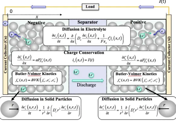
2.4.3 Physics-based methods

These methods are widely used for SOC estimation when the accuracy is the main goal [54], [55]. These methods have intrinsic advantages over traditional Coulomb counting and voltage-based methods. For example, physics-based methods are robust to sensor error and are less dependent on accurate initial SOCs. In physics-based methods, the major problem for real-time SOC estimation is the computational complexity of the coupled partial differential equations (PDEs) which are used to describe the physical processes inside the battery. Simplification of the diffusion PDEs in the solid-phase particles has been found to be the key to reduce the computation time and memory requirement of the physics-based models. The existing methods for diffusion PDE simplification suffer from lots of drawbacks. For instance, the commonly used volume-averaging method can generate unstable equations, which may lead to unacceptable error. Projection-based methods are promising for the model reduction of diffusion PDEs. However, the basis function used in the projection can greatly influence the performance, and how to construct an optimal basis function has not been discussed in the literature. In addition, state filters are required when using a physics-based model for battery SOC estimation. Available state filter algorithms are effective to handle measurement noise and modeling uncertainties. However, these algorithms converge slowly if the initial error is high, which can cause inconvenience to battery users; however, in a recently published papers physics-based electrochemical model is proposed for Li-ion battery SOC estimation involving the battery’s internal physical and chemical properties such as lithium concentrations to solve the computationally complex

25

solid-phase diffusion equations of physical models [56]. An electrochemical model is shown in the following figure

Figure 2.8 Dual-foil battery electrochemical model

2.4.4 Equivalent circuit model (ECM) or Electrical model

The ECM is widely applied to BMS and battery SOC estimation because it is computationally efficient [57], [58]. However, because the ECM is empirical in nature, it provides little insights into the electrochemical process inside the battery, and it cannot provide highly accurate results. It uses electrical circuit components, such as resistors, capacitors, and voltage source to build circuit networks to describe the terminal voltage of batteries. It can describe various dynamic behaviors of the battery accurately. It has good applicability and expansibility, and can be used to develop the model-based SoC estimation approach precisely. Fig.6 presents an ECM with n RC networks, named the NRC model hereafter. The model contains three parts: (i) Voltage source: it uses open circuit voltage

26

(OCV) to denote battery voltage source. (ii) Ohmic voltage cross the equivalent ohmic resistance 𝑅_𝑖, which represents the electrical resistance from various battery components or with the accumulation and dissipation of charge in the electrical double layer. (iii) Dynamic voltage behavior and the mass transport effects: the elements of 𝑅_𝐷 and 𝐶_𝐷 are used to describe the diffusion resistance and diffusion capacitance. 𝐶𝐷𝑖 denotes the 𝑖𝑡ℎ equivalent

diffusion capacitance and 𝑅_𝐷𝑖 denotes the 𝑖_𝑡ℎ equivalent diffusion resistance, 𝑈_𝐷𝑖 is the voltage across 𝐶_𝐷𝑖, i = 1, 2, 3, 4, . . . n [59]. In figure 2.9, 𝑖_𝐿 denotes battery load current, 𝑈_𝑡 denotes battery terminal voltage.

Figure 2.9 Schematic diagram of the NRC ECM [59]

Electrical behavior of the NRC battery model can be expressed by Equation (2.2).

(2.9)

For working BESS in the safe operating area (SOA), there is a BMS block which controls the voltage, current and temperature of the cells. SOA is a window with safe predefined values for the cell voltages, currents, and temperatures where a battery can operate continuously without any harms or damages [60]. BMS deals with an equivalent

27

circuit since it works on-line and prevents the battery from detrimental operation by measuring in real-time both voltage and current at terminals.

It is noted that the symbol of battery current is positive during the discharging process and the symbol is negative for charging process. These electrical models can be quite simple as models that take into account only the static behavior or more complex ones that take into account the dynamic behavior as well [61]. Following are the two main subgroup of the model-based SoC estimation with the ECM:

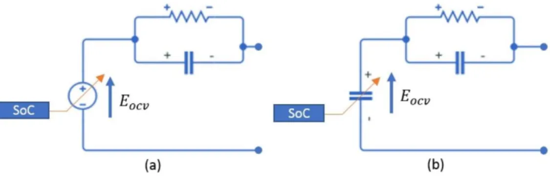
2.4.4.1 Active models

Battery models, in most cases, are composed of a voltage source, whose terminal voltage is a function of the state of charge (SoC), and passive elements, as resistors and capacitors, to model the dynamic behavior of batteries over a certain frequency range [62], [63]. Moreover, these elements can also be functions of other quantities as temperature, current and so on. Figure 10.a shows a simple battery active model.

2.4.4.2 Passive models

supercapacitors are usually modelled using only passive elements as functions of voltage, and possibly, other quantities [64]. In fact, batteries are most of the time modelled as voltage sources because they are seen as dc electric generators, based on chemical phenomena, whilst supercapacitors are seen as large capacitors because their working is based on the charge accumulation phenomenon through the electric field. Even if a battery has chemical reactions, it is electrically equivalent to a big capacitor whose voltage is related to the charge accumulated in chemical way, instead of in electrical way, into the battery itself. For this reason, it is possible to use also for batteries passive models the same as supercapacitors. Figure 10.b shows a simple battery passive model.

28

Figure 2.10 (a) Active, and (b) Passive ECM

2.4.4.3 Empirical

It uses the experimental results of a battery pack without the consideration of cell information [65], [66]. The model of this method can be applied to the existing state estimation algorithms for batteries with ease because the model has a simple model structure which is considered in the trade-off between model accuracy and computational complexity. Battery packs usually consist of hundreds of battery cells connected in series and parallel, including battery packs made up of several battery modules, with each battery module containing multiple battery cells in series, parallel, or series-parallel configuration. Going from battery cell model to battery pack model is not simply aggregating cell models to make a pack model, because in this way not only will it introduce unnecessary computational requirements for system simulation, but also because some phenomena that can only be observed in the battery pack are ignored [67]. Significant fidelity loss will occur if inadequate attention is paid to the battery pack behavior, as opposed to cell-level modeling. Thus, it is worth investigating the construction of a battery pack model separately from the cell model.

Three approaches for battery pack modeling are available in the literatures. The first approach is aggregating cell models in series and parallel to represent the battery pack model [68], [69]. This approach requires the least effort going from the cell model to pack model, as the only information needed is the cell configuration in the battery pack. However, serious

29

loss of fidelity can occur in the resulting battery pack model as a result of ignoring the cell variations, thermal unbalancing in the battery pack, etc. At the same time, in reality not all battery cells used in battery packs are even available to the actual system designers for battery cell modeling.

The second approach is to scale the cell model into a battery pack model with one simplified model representing the battery pack [70], [71]. In this case, the cell discrepancy issues related only to the battery pack are investigated and included in the pack model. Compared with the first approach, the second approach is comprehensive and fast in simulation, which is more suitable for system level design and simulation. Nonetheless, the investigation of cell discrepancy and thermal distribution in a battery pack requires extensive time and effort, and sometimes the battery cells are not readily available to the system designers.

The third approach is building a battery pack model directly on a well-built battery pack with a single battery model capturing the totality of the pack behavior [72], [73]. In this case, the characteristics of the battery cells and thermal influences on them are naturally included into the battery pack model, as a result of cumulative effects of cell averaging, and at the same time the battery model will be fast in simulation requiring comparatively little computational power. Another advantage of this procedure is that non-idealities known to exist in battery packs, such as weak cells and interconnection impedances, is captured self-consistently at the time the battery pack model is built. This approach requires no cell-level details or pack configurations, and some modeling algorithms at this level are even independent of battery chemistry. For commercially available battery packs, this approach may be the only possible approach, as in this case battery tests need only be conducted at the battery pack level. Prerequisites for this approach include 1) the battery cells are reasonably well balanced with means for regular cell balancing, and 2) the battery pack should be effectively cooled/heated so that the battery pack does not encounter uncontrolled temperature variations. In other words, only when a well-designed battery system is available can one confidently model the battery pack as a single battery model. The issue of

30

battery cells variation has been discussed in many papers and communications [70]- [74], and a two-step screening process has been proposed in [70] to ensure a stable configuration of a battery pack, and many cell equalizations approaches have been proposed as well [75], [76]. Comparing the three battery pack modeling approaches discussed above, the third approach which builds a battery pack model directly on battery pack terminal measurements seems to be the most promising for system level designer. However, large modeling errors up to 3.1% for this battery pack modeling approach even with moderate real-world test regimes were reported in the literatures [72], [73], which needs to be improved for stringent high-fidelity system level simulations.

32

Chapter 3

Ancillary Services Market (ASM)

Ancillary Services (AS) is an essential element in any electricity market design. The Independent System Operator (ISO) relies on AS to ensure system security and reliability. AS usually include regulation up (Reg-Up), regulation down (Reg-Down), spinning reserve (Spin), nonspinning reserve (Non-Spin), voltage support, and black start. In some markets, AS products are broken in different categories such as 6 second raise, 6 second lower, 60 second raise and 60 second lower, 30 minutes standby, etc. Operating reserves, i.e., regulation, spin and non-spin, are usually procured through competitive markets. Bidders submit AS bids and then the market clearing price is found as the price where supply is equal to demand. All offers at or below the clearing price are accepted. Voltage support and black start services are usually procured by resource specific agreements between the Independent System Operator (ISO) and the suppliers. A generator must meet certain performance criteria in order to be eligible for providing a specific AS. For example, a generator must be equipped with Automatic Generator Control (AGC) devices in order to provide regulation services. Furthermore, the amount of capacity that a unit can provide is limited by the unit’s operating characteristics, such as ramping capability. The minimum performance requirements for

33

each ancillary service are usually specified by national reliability organizations such as NERC (North America Reliability Council) [77].

3.1 Electricity Market Regulations

The Day-Ahead Market (DAM) is an electricity market that works one day in advance with respect to the actual delivery time. It lets “financial” and “physical” trading. A financial market lets participants to buy or sell energy on the market, with no actual delivery obligation. A financial transfer is related to any energies that is not delivered. On the other side, a physical market related to any trading which is corresponded to an actual transfer of power. The DAM provides both financial and physical participation [78]. The DAM is an auction market and it is not a continuous trading market. It hosts most of the transactions of purchase and sale of electricity. Producers as sellers and consumers as buyers place their offer in an Electricity Pool, which is managed by a central entity called Power Exchange (in Italy, Gestore dei Mercati Energetici - GME). The Power Exchange (PX) represents the only counterparty for the market players, by acting as the only buyer for producers and the only seller for consumers [79]. Note that when buyers and sellers communicate with the PX, they do not know whom they are dealing with.

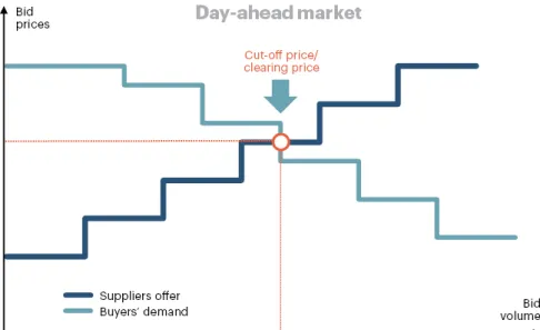
3.1.1 Basic D-ahead market trading principle [80]

- Calculations are made simultaneously for 24 hours of supply for all bids and quotations.

- Prices are set for each hour separately. Equilibrium price is set with the help of special software.

- Pricing principles are as follows:

• Supply and demand curves are formed for each hour of the day in €/MWh. • The intersection of the curves determines the equilibrium price.

34

- Market operator is a central contractor for all sale and purchase deals. Each participant either sells or buys the needed volumes of electricity from the market operator.

- In the Day-ahead market, participants make bids and offers for the purchase and sale of electricity respectively during one or more accounting periods (hours of the day).

- Billing and settlements under agreements are made by the market operator. Figure 3.1 shows the procedure of finding of clearing price (cut-off price) for Day-ahead market:

Figure 3.1 Equilibrium point for Day-ahead market [80]

3.2 Ancillary services

Ancillary services are support, generally referred services other than energy that to those are essential for ensuring the reliable operation of electric power losses, black start capacity, systems [81]. According to this definition, many services such as frequency regulation, voltage regulation, system restoration, load shedding and reserves with varying levels of

35

response time are considered as ancillary services. However, many entities such as Federal Energy Regulatory commission (FERC), North America Electric Reliability council (NERC) and Oak Ridge National Laboratory (ORNL) have developed comprehensive lists of ancillary services [82], [83]. These organizations are related to the USA power system where the nominal frequency for the power systems is 60 Hz. In Europe, the reliability organizations are the national regulatory authorities (NRAs). Transmission System Operator (TSO) is an organization responsible for transporting energy in the form of natural gas or electrical power on a national or regional level, using fixed infrastructure in the Europe. The term is defined by the European Commission. The standard for the nominal frequency for the power systems in Europe is 50 Hz (In the simulation of this work, 50 Hz is the nominal value). TSO in Europe is the same as ISO in the USA.

The power system has metamorphosis in recent years, as a result of the steady growth of renewable energy sources like solar, geothermal, and wind power in the generation mix. Although this brings great advantage as result of its natural eco friendliness, however, unlike, generators, the uncontrollability of RE poses a major challenge to system operators. BESS, on the other hand, is greatly welcomed by system operators because of its advantage of its large energy storage functionality [84]. The enormousness of BESS applications includes, but not limited to: intermittency compensation of renewable energy, frequency regulation, transient stability, voltage support, frequency compensation, frequency regulation, load leveling, spinning reserve, uninterruptable power supply (UPS), and improvement of energy. Although it is most actively developed due to its colossal applications, expensive initial investment cost and limited lifetime are still to its commercialization. However, many such projects are still ongoing for frequency regulation, because of its economic viability [85]. Fast response due to BESS is suitable for frequency regulation and has proven to be superior to existing generators in recent research [86]. In the following, some of the most important ancillary services are explained:

36

3.2.1 Frequency regulation

The system frequency is the heartbeat of the grid. It indicates the balance between power supply and demand of the system. System frequency fluctuations are caused by supply-demand imbalance on the grid. Frequency fluctuations occurs at the instance of sudden power fluctuation. System frequency and demand power shows high correlation at every instance in time. As shown in Figure 3.2, at any given time period, system frequency depicts an inverse proportion with demand power. This is as a result the frequency falls when the demand power rises and the frequency rises when the demand power falls. So, If the balance between generation and demand is not reached, the system frequency will change at a rate initially determined by the inertia of the total system. The total system inertia comprises the combined inertia of most of the spinning generation and load connected to the power system [87]. It should be note that even though the nominal frequency of the Figure 3.2 is 60 Hz, the nominal frequency chosen for the simulation in this work is 50 Hz.

Figure 3.2 Frequency variation vs. demand power [88]

Low levels of rotational inertia in a power system, caused in particular by high shares of inverter-connected renewable energy sources (RES), i.e. wind turbines, and PV panels which normally do not provide any rotational inertia, have implications on the grid’s frequency dynamics. This can lead to situations in which traditional frequency control schemes become too slow with respect to the disturbance dynamics for preventing large frequency deviations and the resulting consequences.

37

The loss of rotational inertia, and its increasing time-variance, leads to new frequency instability phenomena in power systems. Frequency and power system stability may be at risk. If, during a system frequency disturbance, the balance between generation and demand is not maintained, the system’s frequency will change at a rate initially determined by the total system’s inertia. The total system’s inertia comprises the combined inertia of most of the spinning generation and load connected to the power system. The contribution of system inertia of a load or generator is dependent on whether the system frequency causes changes in its rotational speed and, therefore, its kinetic energy. The power associated with this change in kinetic energy is fed by, or taken from, the power system and is known as the “inertial response” [89]. Figure 3.3 shows the typical inertial response requirements of a grid.

Figure 3.3 Grid inertial response [90]

During a system frequency event the total inertial response of all electrical machines connected to the system determines the initial rate of change of frequency (ROCOF).

For a robust power system (system frequency is not overly sensitive to power imbalances), it is extremely important that a large proportion of generation and load connected to the power system contributes to the system’s total inertia and then provides inertia response.

38

Inertial power rating and energy will depend on what is required by the network, and is dependent on the level of power to be supplied to the network in the instant between failure and adjustment of remaining plant to take up the load. The control of a large power system is hierarchical. In this discussion, three frequency control services (primary control, secondary control, and tertiary control) are explained, but our focus is on primary control action.

3.2.1.1 Primary Control Reserve (PCR)

Transient imbalances between generation and consumption induce deviations of the frequency. The main purpose of primary frequency control (PFC) is to react within a few seconds to any frequency deviation higher than ±20mHz to keep frequency variation within the maximum threshold (±200mHz) and re-establish the balance between produced and consumed energy. Currently detection of these deviations is used to tune generators (that participate to this primary frequency control) according to their available power reserve. The same control function can be implemented into the control system of the grid connected power converter, which is embedded in the BESS. From an economic point of view the interest is that the revenue from this given service is constant and warrantied [91].

Load frequency control (LFC) is a term applied to describe the continuous operation of keeping the frequency of a power system stable. The frequency of a power system is connected to the balancing of produced and consumed power in the way that if there is a surplus of produced power the frequency will rise, and if there is a lack of produced power the frequency will fall. It is very important that this power balance is maintained, if not the generators could lose synchronism, and the power system would collapse. As shown in Figure 3.4,LFC has a hierarchical structure with primary and secondary, and tertiary control.

39

Figure 3.4 Activation of primary, secondary, and tertiary control after a power imbalance [92].

PCR acts as follow:

1. In case of under frequency, positive reserve injects power in the grid.

2. In case of over frequency, negative reserve absorb power from grid. Actually, all relevant units inject less power than programmed in grid.

The final goal for PCR is to achieve:

∑ 𝐸_{𝑝𝑟𝑜𝑑𝑢𝑐𝑒𝑑} = ∑ 𝐸_{𝑐𝑜𝑛𝑠𝑢𝑚𝑒𝑑} (3.1) Which means the frequency of the grid gets its optimal initial value (50Hz or 60Hz). PCR is a mandatory service which has to be provided by every production units with apparent power greater than 10MVA. These units are called Relevant Production Units

40

(RPU). PCR is not subject to ASM, but it is remunerated according to the price of electricity in that zone.

3.2.1.1.1 The BESS Controller

In this study, designing of a new controller is not the case. Within this framework, the controller is only used for:

• directly receiving the power setpoints (𝑃gridAC) from input time-series. This occurs

during the verification, where the BESS model must operate on a cycle of the user’s choice;

• converting frequency deviation into a power setpoint via a droop control curve. This occurs during the validation process, where the BESS model is tested via frequency regulation cycles. The droop control curve is built in the model controller based on the curve controlling the operation of a real battery under study while providing frequency regulation. It is a simplified control curve, defined in Equation (3.2) and presented in Figure 4.5, featuring no dead band and a droop value of 0.69%. The utilization of a droop curve without a dead band could be a decrement in the test duration due to the its incrementation in energy flow during the test. This is suitable for the validation process since its purpose is to investigate the estimation error rather than the effectiveness of the control strategy. computed as follows: 𝑑𝑟𝑜𝑜𝑝 = − 𝑑𝐹 𝐹_𝑛 𝑑𝑃 𝑃𝑛 × 100 [%] (3.2)

where dF is the frequency deviation (in Hz), Fn is the network nominal frequency of 50 Hz, dP is the power setpoint (in kW), and Pn is the nominal power of BESS (in kW).

41

3.2.1.2 Secondary Control Reserve (SCR)

Secondary frequency control, also referred to as load frequency control (LFC), is the second level for compensating an active power mismatch. After PCR reached to its maximum power delivery, SCR starts and must achieve to its nominal value within 15 minutes. If it does not, tertiary control takes over from secondary control. As opposed to primary control, secondary control reacts only to a disturbance in the LFC’s own control area in order not to change the load flows on tie-lines to other areas. It can be either performed manually or automatically. PCR can only interrupts deviation and reach to a steady-state frequency value which is higher or lower, depending on the situation, than the nominal value. It cannot restore frequency to the optimal nominal value. SCR causes an unbalance in grid for a certain period of time. It is injecting power if frequency is below the nominal value and absorbing power in case frequency is above nominal value.

SCR is not mandatory, and each provider is required to have high power set points as the number of providers are not many. They must offer the same power band for positive and negative reserve: SCR is a symmetric service. In order to avoid any constraints, TSO given the total available quantity of PCR and calculates the total power required to restore the nominal value of frequency and shares it among all the providers. In Italy, the TSO

42

defines each minute a signal, called Area Control Error (ACE - Livello Regolazione Secondaria is the Italian name), which is valid simultaneously for all providers. It represents the percentage of power reserve required to each production unit selected in the market [93]. The scale for the ACE signal is a number between 0 and 100 [94].

{

∆𝑃 = ∆𝑃_𝑆𝐶𝑅 𝑖𝑓 𝐴𝐶𝐸 = 100 ∆𝑃 = 0 𝑖𝑓 𝐴𝐶𝐸 = 50 ∆𝑃 = −∆𝑃𝑆𝐶𝑅 𝑖𝑓 𝐴𝐶𝐸 = 0

(3.3)

3.2.1.3 Tertiary Control Reserve (TCR)

It also known as manual frequency restoration reserve (mFRR), frequency restoration reserves (FRR), and replacement reserves (RR). In case of necessity, tertiary control reserves are manually activated within 15 min by the TSO. It is primarily activated to free secondary reserves in a balanced situation, but also to support secondary control after a large incident to restore the frequency to the nominal value and prevent the need of primary control. Tertiary control reserves have to run until the generation is re-scheduled to fit the new system situation [92].

In Italy, this service is centrally coordinated by Terna and traded on Ancillary Services Market. It requires slower but longer action (as shown in Figure 3.4); hence, it has a slow ramp and a large energy output.

3.2.2 Voltage Control

Distribution networks have not been designed to cope with power injections from Distributed grid (DG), therefore the proliferation of DG on the electric networks results in a number of adverse impacts, including voltage variation, degraded protection, altered transient stability, bi-directional power flow and increased fault level, the voltage variation

43

has been addressed as the dominant effect [95]. Typically, one of the most severe situations is that voltage magnitude at the proximity of DG exceeds the statutory limits during maximum power output from DG and minimum power demand from the network. Here the network experiences the largest reverse power flow and large voltage change which affects the network safety and stability.

Distribution network operators (DNOs) are responsible for operating the network within statutory limits. The voltage variation problem can be solved by either network, generator or load operational changes (utilizing the existing infrastructure) or network asset upgrades [95]. The network and generator operational changes, such as DG power curtailment, may conflict with contractual policies (“first on last off”) between DNOs and DG. Whilst the network asset upgrades, such as reinforcement of networks, require significant investments on the distribution networks. DNOs need to justify the cost in terms of revenue benefit [96].

3.2.3 System Restoration

The objectives of restoration are to enable the power system to return to normal conditions securely and rapidly, minimize losses and restoration time, and diminish adverse impacts on society. Many non-structured methods and technologies and object-oriented expert system have been employed in making restoration schemes to address the above objectives, but the establishment and maintenance of a knowledge base of past restorations remains a bottleneck [97].

Wind and solar power as clean and renewable energy are significantly adopted but they are inherently volatile, intermittent and random. Therefore, an improper handling of certain partial failures can easily lead to accidents and severe chain reactions, and thus may cause large-scale/extensive blackout eventually. Large-scale blackout risks still exist and are inevitable, although a great amount of work has been done to make power systems resilient against outages [98]. A proper restoration plan can effectively mitigate the negative impact

44

on the public, the economy, and the power system itself. Research on how to restore the power system quickly and effectively after outages is of vital significance.

Power system restoration after a partial or complete collapse is quite a complex process. Many factors need to be considered including the operating status of the system, the equipment availability, the restoration time and the success rate of operation. It needs not only a large amount of analysis and verification, but also decisions made by dispatching personnel. Power system restoration is a multi-objective, multi-stage, multi-variable and multi-constraint optimization issue, and is full of non-linearity and uncertainty. It can be described as a typical semi-structured decision-making and it is difficult to obtain a complete solution [99].

3.3 BESS for Ancillary Services Provision

In the Nordic Network, the TSOs aim at keeping the frequency between 49.9 and 50.1 Hz. This has proven to be increasingly difficult, and as seen from Figure 3.6,the number of frequency incidents (minutes spent outside 49.9 and 50.1 Hz) has increased concurrently with installed wind power capacity over the last decade. It is confirmed by Statnett, the Norwegian TSO, that the increasing amount of intermittent energy resources is part of the reason for the decreasing control performance, along with a heavier loaded network and an increasing amount of bottlenecks, which at times excludes some of the resources from participating in LFC [100]. There have been many suggestions to how LFC can be improved to better cope with these challenges. In some literatures, loads are included in LFC [101], [102], while [103] concentrated on effective energy storage. BESS can absorb energy during periods of high frequency and dispatch energy during periods of low frequency. A fairly complex control algorithm is required to ensure that the BESS is capable of performing either function when required [90].

Energy support for frequency management is short in nature and many solutions are based on super- and ultra-capacitors. Ultra-capacitors are well-suited to supply as such a