A hybrid autotuning framework for performance optimization of heterogeneous systems

(1)

POLITECNICO DI MILANO

Corso di Laurea Magistrale in Ingegneria Informatica Dipartimento di Elettronica, Informazione e Bioingegneria

A Hybrid Autotuning Framework for

Performance Optimization of

Heterogeneous Systems

Advisor:

Prof. Cristina Silvano Co-Advisor:

Prof. Gianluca Palermo Dr. Amir H. Ashouri

Master Thesis of:

Mahdi Fani-Disfani (841258) Puya Amiri (835886)

(2)

(3)

Abstract in English

The increasing complexity of modern multi and manycore hardware design makes performance tuning of the applications a difficult task. While the aid of the successful past automatic tuning has been the execution time minimization, the new performance objectives have emerged comprise of energy consumption, computational cost, and area.

Automatic Tuning approaches range from the relatively non-intrusive (e.g., by using compiler options) to extensive code modifications that at-tempt to exploit specific architectural features. Intrusive techniques often result in code changes that are not easily reversible, which can negatively impact readability, maintainability, and performance on different architec-tures.

Therefore, more sophisticated methods capable of exploiting and identi-fying the trade-offs among these goals are required. We introduce a Hybrid Optimization framework to optimize the code for two main mutually com-peting criteria, e.g., execution time and resource usage in several layers starting from the original source code to a high-level synthesis level. Several effective tools and optimizations are involved, i.e., OpenTuner framework for building domain-specific multi-objective program autotuners, Annotation-based empirical tuning system called Orio, and a high-level synthesis tool named LegUp are the optimization components of our framework. The framework aims at improving both performance and productivity over a semi-automated procedure.

Our chain supports both architecture-independent and architecture-specific code optimization and can be adapted to any hardware platform architec-ture. After identifying the application’s optimization parameters through OpenTuner, we pass the annotated code as input to Orio which generates many tuned versions and returns the version with the best performance. Furthermore, LLVM performs a number of optimization passes according to the Orio’s result and finally, LegUp will use the LLVM output to synthesis for a particular target platform adding its optimizations.

We show that our automated approach can improve the execution time and resource usage on HLS through different optimization levels.

(4)

(5)

Sommario

La crescente complessit`a del moderno design hardware multi e manycore rende l’ottimizzazione delle prestazioni delle applicazioni un compito diffi-cile. Mentre l’aiuto della sintonizzazione automatica conclusa con successo `

e stata la riduzione dei tempi di esecuzione, sono emersi i nuovi obiettivi di prestazione che comprendono il consumo di energia, il costo computazionale e l’area.

Gli approcci di ottimizzazione automatica spaziano dal relativamente non intrusivo (ad esempio, utilizzando le opzioni del compilatore) alle es-tese modifiche del codice che tentano di sfruttare specifiche caratteristiche architettoniche. Le tecniche intrusive spesso portano a modifiche del codice che non sono facilmente reversibili, il che può avere un impatto negativo sulla leggibilit Ã , sulla manutenibilità e sulle prestazioni su diverse architetture.

Pertanto, sono necessari metodi pi`u sofisticati in grado di sfruttare e identificare i trade-off tra questi obiettivi. Introduciamo una struttura di ottimizzazione ibrida per ottimizzare il codice per due criteri principali che si confrontano reciprocamente, ad es. Tempo di esecuzione e utilizzo delle risorse in diversi livelli, a partire dal codice sorgente originale fino ad un liv-ello di sintesi di alto livliv-ello. Sono coinvolti diversi strumenti e ottimizzazioni efficaci, ovvero il framework OpenTuner per la creazione di autotuner di programmi multi-obiettivo specifici del dominio, il sistema di ottimizzazione empirica basato su Annotation chiamato Orio e uno strumento di sintesi di alto livello denominato LegUp sono i componenti di ottimizzazione del nostro framework . Il framework mira a migliorare sia le prestazioni che la produttivit`a attraverso una procedura semi-automatica.

La nostra catena supporta l’ottimizzazione del codice indipendente dall’ architettura e l’architettura specifica e pu`o essere adattata a qualsiasi ar-chitettura di piattaforma hardware. Dopo aver identificato i parametri di ottimizzazione dell’applicazione tramite OpenTuner, passiamo il codice an-notato come input a Orio che genera molte versioni ottimizzate e restituisce la versione con le migliori prestazioni. Inoltre, LLVM esegue un numero di passaggi di ottimizzazione in base al risultato di Orio e, infine, LegUp uti-lizzer`a l’output LLVM per la sintesi di una determinata piattaforma target aggiungendo le sue ottimizzazioni.

(6)

tempi di esecuzione e l’utilizzo delle risorse su HLS attraverso diversi livelli di ottimizzazione.

(7)

Acknowledgement

This Master of Science thesis has been carried out at the Department of Electronics and Computer (DEIB) at Politecnico di Milano University. The work has been performed within the HEAP laboratory of professors Cristina Silvano and Gianluca Palermo.

Being part of HEAP was a great and an invaluable experience. We take many memorable and enjoyable moments we spent with our colleagues while investigating the state-of-the-art problems. We thrived from all the moments and would like to appreciate all our teammates there.

First and foremost, we would very much like to thank our supervisors at Politecnico di Milano, Cristina Silvano and Gianluca Palermo who always had the answer to our questions and guided us towards the right way. Their constant encouragement and support throughout the project made it possi-ble for us to complete the work.

We would also like to thank Dr. Amir H. Ashouri, a former Ph.D. student of HEAP and a current postdoctoral researcher at University of Toronto, Canada; It was a pleasure having his advice and excellent experiences in the field of computer architecture especially, compiler field.

Moreover, we would like to appreciate lifetime support of our perfect fami-lies whom always been there for us during the hard-times and good-times. Thank you so much for stop-less giving us the positive energy to carry-on and thanks for urging us to choose this path for our life.

Finally, we would like to thank everyone in Politecnico di Milano University circle, from our colleagues, secretaries to the professors, who got involved in such a way to let this checkpoint of our life happens.

(8)

(9)

5.4.1 Result Tables . . . 75 5.4.2 Performance Diagrams . . . 76 5.5 DFMUL Benchmark . . . 78 5.5.1 Result Tables . . . 79 5.5.2 Performance Diagrams . . . 79 5.6 GSM Benchmark . . . 82 5.6.1 Result Tables . . . 83 5.6.2 Performance Diagrams . . . 83 5.7 DFADD Benchmark . . . 86 5.7.1 Result Tables . . . 86 5.7.2 Performance Diagrams . . . 88 5.8 ADPCM Benchmark . . . 90 5.8.1 Result Tables . . . 91 5.8.2 Performance Diagrams . . . 91 5.9 MIPS Benchmark . . . 94 5.9.1 Result Tables . . . 94 5.9.2 Performance Diagrams . . . 95 5.10 DFDIV Benchmark . . . 97 5.10.1 Result Tables . . . 97 5.10.2 Performance Diagrams . . . 100 5.11 DFSIN Benchmark . . . 102 5.11.1 Result Tables . . . 102 5.11.2 Performance Diagrams . . . 103 5.12 JPEG Benchmark . . . 105

(11)

5.12.1 Result Tables . . . 105

5.12.2 Performance Diagrams . . . 107

6 Conclusion and Future Works 111 6.1 Conclusion . . . 111

6.2 Future Works . . . 112

Bibliography 115 A Mandelbrot 121 B Loop Transformation Modeling 141 B.1 Source to Source Transformation . . . 141

B.2 Theory of code transformation . . . 142

B.2.1 Polyhedral Model for nested loops . . . 142

B.3 Loop Transformation . . . 144 C Codes 147 C.1 AXPY . . . 147 C.2 ADPCM . . . 149 C.3 DFADD . . . 151 C.4 DFMUL . . . 156 C.5 DFSIN . . . 159 C.6 DFDIV . . . 163 C.7 GSM . . . 167 C.8 MIPS . . . 168 C.9 JPEG . . . 170 C.10 Matrix Multiplication . . . 173 C.11 Bash Scripts . . . 175

(12)

(13)

List of Figures

1.1 Mandelbrot Area Delay on different HLS approaches . . . 4

1.2 Hybrid Optimization Framework Overview . . . 6

2.1 Extraction of addition loop into datapath and control logi-chow transformations affect the hardware implementation. . 11

2.2 Consecutive loops for addition and multiplication within a function . . . 13

2.3 Merged addition and multiplication loops . . . 14

2.4 Example code for nested loops adding the elements of two dimensional arrays . . . 14

2.5 Control flow through the matrix addition, without flattening (clock cycles in circles) . . . 16

2.6 Overview of Orio’s code generation and empirical tuning pro-cess. . . 18

2.7 Integration of Pluto and Orio . . . 19

2.8 OpenTuner structure . . . 21

2.9 OpenTuner components . . . 21

2.10 LegUp Design Flow . . . 24

2.11 Target System Architecture . . . 24

2.12 Design flow with legup . . . 26

2.13 MIPS datapath with control unit. . . 28

2.14 Terasic , DE1 SoC . . . 30

2.15 Altera’s Cyclon V SoC Architecture . . . 31

3.1 ASV triangles for the conventional and auto-tuned approaches to programming. . . 34

3.2 High-level discretization of the autotuning optimization space. 34 3.3 Visualization of three different strategies for exploring the optimization space: (a) Exhaustive search, (b) Heuristically-pruned search, and (c) hill-climbing. Note, curves denote combinations of constant performance. The gold star repre-sents the best possible performance. . . 35

(14)

3.4 Comparison of traditional compiler and autotuning capabil-ities. Low-level optimizations include loop transformations

and code generation.†only via OpenMP pragmas. . . 36

4.1 Methodology Diagram . . . 43

4.2 HOF Tool Chain . . . 44

4.3 Methodology Diagram, first section . . . 46

4.4 Methodology Diagram, second section . . . 48

5.1 Brief description and source of the CHStone benchmark pro-grams [1]. . . 53

5.2 Source-level characteristics [1]. . . 54

5.3 The number of states and resource utilization in RTL descrip-tion [1]. . . 55

5.4 Pareto Curve . . . 56

5.5 Graphical interpretation of blocked matrix multiply The in-nermost (j, k) loop pair multiplies a 1 ∗ bsize sliver of A by a bsize ∗ bsize block of B and accumulates into a 1 ∗ bsize sliver of C . . . 58

5.6 The BWMM Wall-Clock Time diagram of the original code vs. different optimization levels . . . 66

5.7 BWMM Speedup w.r.t baseline . . . 67

5.8 BWMM Logic Utilization Efficiency w.r.t baseline . . . 67

5.9 Area Delay of baseline vs. HOF . . . 68

5.10 BWMM cache miss rate w.r.t baseline . . . 69

5.11 BWMM different phases speedup . . . 70

5.12 BWMM different phases logic utilization efficiency . . . 71

5.13 BWMM different phases Area Delay . . . 71

5.14 AXPY Speedup diagram . . . 73

5.15 AXPY logic utilization efficiency diagram . . . 74

5.16 AXPY Area Delay diagram . . . 74

5.17 Matrix Multiply Speedup diagram . . . 76

5.18 Matrix Multiply Utilization diagram . . . 77

5.19 Matrix Multiply Area Delay diagram . . . 77

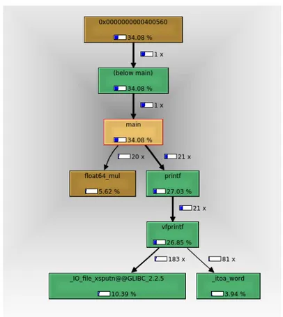
5.20 DFMUL Profiling. The Call-graph depicting calling relation-ships and computational needs of each function . . . 78

5.21 DFMUL Speedup diagram . . . 80

5.22 DFMUL Utilization diagram . . . 81

5.23 DFMUL Area Delay diagram . . . 81

5.24 GSM Profiling. The Call-graph depicting calling relationships and computational needs of each function . . . 82

5.25 GSM Speedup diagram . . . 84

5.26 GSM Utilization diagram . . . 85

(15)

5.28 DFADD Profiling. The Call-graph depicting calling

relation-ships and computational needs of each function. . . 86

5.29 DFADD Speedup diagram . . . 88

5.30 DFADD Utilization diagram . . . 89

5.31 DFADD Area Delay diagram . . . 89

5.32 ADPCM Profiling, ADPCM Call-graph depicting calling re-lationships and computational needs of each function . . . 90

5.33 ADPCM Speedup diagram . . . 92

5.34 ADPCM Utilization diagram . . . 93

5.35 ADPCM Area Delay diagram . . . 93

5.36 MIPS Profiling, the Call-graph depicting calling relationships and computational needs of each function . . . 94

5.37 MIPS Speedup diagram . . . 96

5.38 MIPS Utilization diagram . . . 96

5.39 MIPS Area Delay diagram . . . 97

5.40 DFDIV Profiling, The Call-graph depicting calling relation-ships and computational needs of each function . . . 98

5.41 DFDIV Speedup diagram . . . 100

5.42 DFDIV Utilization diagram . . . 101

5.43 DFDIV Area Delay diagram . . . 101

5.44 DFSIN Profiling. The call-graph depicting calling relation-ships and computational needs of each function . . . 102

5.45 DFSIN Speedup diagram . . . 104

5.46 DFSIN Utilization diagram . . . 104

5.47 DFSIN Area Delay diagram . . . 105

5.48 JPEG Profiling. The Call-graph depicting calling relation-ships and computational needs of each function . . . 106

5.49 JPEG Speedup diagram . . . 108

5.50 JPEG Utilization diagram . . . 108

5.51 JPEG Area Delay diagram . . . 109

6.1 Normalized Execution Time of All Benchmarks w.r.t Baseline 112 6.2 Speedup of all benchmarks besides their corresponding logic utilization efficiency w.r.t original . . . 113

A.1 Pareto Curve . . . 124

A.2 Mandelbrot call graph . . . 126

A.3 Mandelbrot scheduling details . . . 127

A.4 Loop Pipelining . . . 127

A.5 Loop Pipelining Scheduling . . . 129

A.6 Schedule for loop lp1 in the transformed Mandelbrot code. . . 133

A.7 Mandelbrot Fmax on different HLS approaches . . . 136

A.8 Mandelbrot Wall Clock Time on different HLS approaches . . 137

(16)

A.10 Mandelbrot Clock cycles on different HLS approaches . . . . 138 A.11 Mandelbrot DSP blocks on different HLS approaches . . . . 139 A.12 Mandelbrot Area*Delay on different HLS approaches . . . . 139 A.13 Mandelbrot ALMs on different HLS approaches . . . 140 B.1 An Example of Array Access Pattern . . . 143 B.2 An An example of column access pattern. There are 4

pat-terns with different traverse directions. . . 143 B.3 An example of diagonal access pattern with slope = 1. There

(17)

List of Tables

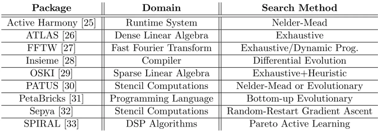
3.1 Summary of selected related projects using autotuning . . . . 37

5.1 OpenTuner in HLS Framework . . . 65

5.2 Pure Hardware AXPY HLS Analysis . . . 72

5.3 Pure Software AXPY HLS Analysis . . . 72

5.4 Hardware/Software AXPY HLS Analysis . . . 73

5.5 Pure Hardware Matrix Multiply HLS Analysis . . . 75

5.6 Pure Software Matrix Multiply HLS Analysis . . . 75

5.7 Hardware/Software Matrix Multiply HLS analysis . . . 76

5.8 Pure Hardware DFMUL HLS Analysis . . . 79

5.9 Pure Software DFMUL HLS Analysis . . . 79

5.10 Hardware/Software DFMUL HLS Analysis . . . 80

5.11 Pure Hardware GSM HLS Analysis . . . 83

5.12 Pure Software GSM HLS Analysis . . . 83

5.13 Hardware/Software GSM HLS Analysis . . . 84

5.14 Pure Hardware DFADD HLS Analysis . . . 87

5.15 Pure Software DFADD HLS Analysis . . . 87

5.16 Hardware/Software DFADD HLS Analysis . . . 87

5.17 Pure Hardware ADPCM HLS Analysis . . . 91

5.18 Pure Software ADPCM HLS Analysis . . . 91

5.19 Hardware/Software ADPCM HLS Analysis . . . 92

5.20 Pure Hardware MIPS HLS Analysis . . . 95

5.21 Pure Software MIPS HLS Analysis . . . 95

5.22 Pure Hardware DFDIV HLS Analysis . . . 99

5.23 Pure Software DFDIV HLS Analysis . . . 99

5.24 Hardware/Software DFDIV HLS Analysis . . . 100

5.25 Pure Hardware DFSIN HLS Analysis . . . 103

5.26 Pure Software DFSIN HLS Analysis . . . 103

5.27 Pure Hardware JPEG HLS Analysis . . . 107

5.28 Pure Software JPEG HLS Analysis . . . 107

A.1 Mandelbrot HLS Analysis . . . 122

(18)

C.2 Three sets of favourable LLVM-opt flags for blowfish . . . 183 C.3 Three sets of favourable LLVM-opt flags for dfadd . . . 184

(19)

Listings

2.1 Example code for a loop adding the elements of two arrays . 11

5.1 BWMM original code . . . 58

5.2 Autotuner program for OpenTuner to find optimum parame-ters for BWMM . . . 59

5.3 Annotated BWMM . . . 60

5.4 BWMM Orio transformation specification . . . 61

5.5 BWMM tuned and transformed code . . . 62

A.1 Mandelbrot Kernel . . . 123

A.2 Transformed Mandelbrot Kernel . . . 130

A.3 Threaded Mandelbrot Kernel . . . 132

C.1 Annotated AXPY code . . . 147

C.2 AXPY Orio specification code to use for S2S transformation . 147 C.3 Tuned and transformed AXPY code after S2S transformation by Orio . . . 148

C.4 Annotated ADPCM code . . . 149

C.5 ADPCM Orio specification code to use for S2S transformation 149 C.6 Tuned and transformed ADPCM code after S2S transforma-tion by Orio . . . 150

C.7 Annotated DFADD code . . . 151

C.8 DFADD Orio specification code to use for S2S transformation 151 C.9 Tuned and transformed DFADD code after S2S transforma-tion by Orio . . . 152

C.10 Annotated DFMUL code . . . 156

C.11 DFMUL Orio specification code to use for S2S transformation 156 C.12 Tuned and transformed DFMUL code after S2S transforma-tion by Orio . . . 157

C.13 Annotated DFSIN code . . . 159

C.14 DFSIN Orio specification code to use for S2S transformation 160 C.15 Tuned and transformed DFSIN code after S2S transformation by Orio . . . 160

C.16 Annotated DFDIV code . . . 163

C.17 DFDIV Orio specification code to use for S2S transformation 163 C.18 Tuned and transformed DFDIV code after S2S transforma-tion by Orio . . . 164

(20)

C.19 Annotated GSM code . . . 167

C.20 GSM Orio specification code to use for S2S transformation . 167 C.21 Tuned and transformed GSM code after S2S transformation by Orio . . . 168

C.22 Annotated MIPS code . . . 169

C.23 MIPS Orio specification code to use for S2S transformation . 169 C.24 Tuned and transformed MIPS code after S2S transformation by Orio . . . 169

C.25 Annotated JPEG code . . . 170

C.26 JPEG Orio specification code to use for S2S transformation . 171 C.27 Tuned and transformed JPEG code after S2S transformation by Orio . . . 171

C.28 Annotated Matrix Multiplication code . . . 173

C.29 Matrix Multiplication Orio specification code to use for S2S transformation . . . 173

C.30 Tuned and transformed Matrix Multiplication code after S2S transformation by Orio . . . 174

C.31 GUI and command line tool for the main chain tests . . . 175

C.32 GProf profiler . . . 178

C.33 Perf profiler . . . 179

C.34 Valgrind profiler . . . 180

(21)

(22)

Chapter 1

Introduction

The performance of a software application crucially depends on the quality of its source code. The increasing complexity and multi/many-core nature of hardware design have transformed code generation, whether done manually or by a compiler, into a complex, time-consuming, and error-prone task which additionally suffers from a lack of performance portability [2].

To mitigate these issues, a new research field, known as autotuning, has gained increasing attention. Autotuners are an effective approach to generate high-quality portable code. They produce highly efficient code versions of libraries or applications by generating many code variants which are evaluated on the target platform, often delivering high-performance code configurations which are unusual or not intuitive [2].

1.1 Motivation

Earlier autotuning approaches were mainly targeted at improving the exe-cution time of a code [3]. However, recently other optimization criteria such as energy consumption or computing costs are gaining interest. In this new scenario, a code configuration that is found to be optimal for low execution time might not be optimal for another criterion or vice-versa.

Therefore, there is no single solution to this problem that can be con-sidered optimal, but a set, namely the Pareto set, of solutions (i.e., code configurations) representing the optimal trade-off among the different opti-mization criteria. Solutions within this set are said to be non-dominated: any solution within it is not better than the others for all the considered criteria.

This multi-criteria scenario requires a further development of autotuners, which must be able to capture these trade-offs and offer them using either the whole Pareto set or a solution within it. Although there is a growing amount of related work considering the optimization of several criteria [4, 5, 6, 7, 8], most of them consider two criteria simultaneously at most, and many fail in

(23)

capturing the trade-off among the objectives.

There is two factor in common to most of these autotuning methods and frameworks, first is that they focus exclusively on a single optimization technique and objective such as execution time, memory behavior or resource consumption. Only little support exists for code optimizers that deal with trade-offs between multiple, conflicting goals. Second, they do not consider the effect of optimization mixture in different application execution levels from software code to hardware synthesis; in particular, the effect of loop transformation on HLS which has been highlighted as the most effective optimization in Mandelbrot set [9] benchmark. The Mandelbrot set and the result of performance evaluation of different possible HLS optimizations is extensively described in Appendix A.

Figure A.12 shows a key plot that motivates the proposed framework in this thesis. Taking into account the importance of Area-Delay (indicat-ing the combination of execution time an resource consumption), the figure shows that Loop Transformations or generally Code Transformations yields the best Area-delay product meaning that the concept of source to source compilation to reform the programming structure not only affects in the context of sequential software but also extremely impacts on High-Level Synthesis and subsequent circuitries in terms of area and speed.

Figure 1.1: Mandelbrot Area Delay on different HLS approaches

In this thesis, we introduce a novel multi-objective hybrid optimization framework to optimize two different criteria: execution time, resource usage. The basic idea is to integrate different tools and semi-automatically find an effective set of optimizations with proper parameter settings (e.g., tile sizes

(24)

and unrolling factors) for individual code regions. It is based on the ap-plication parameter tuning, Source-to-Source transformation, compiler and High-Level Synthesis optimizations. We examine the obtained results in detail by analyzing and illustrating the interaction between software opti-mizations and hardware synthesis. Our approach is generic and can be ap-plied to arbitrary transformations and parameter settings. We demonstrate our implementation by exploring the trade-off between execution time and resource efficiency when tuning loop transformations applied.

1.2 Contribution

Our method, which is based on a combination of software level optimizations and hardware level optimization techniques, is described in chapter 3. In this section, we illustrate an overview of our solution, highlighting the five main components: the code analyzer and profiler, application parameter autotuning, source-to-source code transformation, compiler Optimizations and the HLS optimization techniques. Each of them can be individually customized or exchanged by alternative implementations.

The labels in Figure 1.2 follow the processing of a program within our framework. An input code will be loaded by our Profiler Valgrind, analyzed and autotuned by application parameter autotuner. Then annotated by S2S coded transformer Orio, transformed and passed to our compiler LLVM to optimize and used as the input of the HLS with further optimization before synthesis.

For the region of the hot function which is the most time intensive part of the application found by the profiler, the application parameter autotuner determines the best value for the candidate parameters. The autotuned code will be annotated and transformed by the source-to-source code transformer which describes generic sequences of code transformations using unbound parameters for tunable properties (e.g., tile sizes, unrolling factors or vec-torization). The associated transformation skeletons and some (optional) parameter constraints, will be evaluated (executed) on the target system automatically by the transformer and the best transformation with chosen parameter configuration is passed on to the compiler. At this point, the com-piler conducts code optimization by using efficient comcom-piler flags iteratively selecting standard sets of flags. After the compilation flow, corresponding to the target architecture for synthesis, some High-Level Synthesis optimiza-tions will be applied to the code through synthesis tool.

In the end, our framework will generate the report including details regarding the represented trade-off between execution time and resource us-age of the input application with the optimized code and its optimization configuration in each step which is application specific and architectural-dependent. However, the ultimate method to utilize automatically all the

(25)

Figure 1.2: Hybrid Optimization Framework Overview

steps of the framework and gained the opportunity of dynamically customiz-ing attributes and uscustomiz-ing better strategy to choose compiler flags like machine learning is beyond the scope of this thesis and left for future research. The major contributions of this work include:

• The design of a novel hybrid optimization framework facilitating the consideration of multiple conflicting criteria simultaneously by passing through a multi-objective optimization chain

• The combination of the application parameter tuning and the search for optimal loop transformation to minimize execution time and re-source usage efficiency

• The development of a hybrid optimization framework capable of solv-ing the combined problem ussolv-ing an effective number of optimization steps

1.3 Thesis Outline

(26)

• In Chapter 2 there is the description of the background and the exter-nal tools and frameworks on which this work is based on. It introduces related concepts and works, and target architecture of this thesis. • Chapter 3 gives an overview of the state-of-the-art regarding

method-ologies and techniques developed in this thesis, focusing on the de-scription of the OpenTuner autotuner, Orio S2S transformer, and the LegUp HLS framework.

• In Chapter 4 there is the detailed description of the framework im-plemented, in terms of components and behavior. We describe the methodology proposed step by step and the logic structure developed for building Hybrid Optimization Framework.

• In Chapter 5 contains all the experiments we made to validate our proposed methodology and to gather information on the framework behavior.

• Chapter 6 contains the conclusions of this work, with the description of both benefits and limitations, and the list of possible future works that can be done in order to improve and expand this thesis.

• Appendix A elaborates Mandelbrot algorithm and evaluates the per-formance of different synthesis approaches. The results explain the main motivation behind proposing the framework.

• Appendix B is about modeling the transformations. As the PluTo integrated into Orio implements loop transformations based on poly-hedral modeling, also taking into account various loop optimizations that can be enabled by LLVM opt command, in this appendix we describe the theory of source code optimization techniques.

• Appendix C covers almost all the codes used for experiments, exclud-ing the unmodified baselines1. There you can find annotated codes, specifications, Tuned codes and framework scripts.

Finally, there is the bibliography.

1_{Original unmodified codes}

(27)

(28)

Chapter 2

Background

The size and complexity of scientific computations are increasing at least as fast as the improvements in processor technology. Programming such scientific applications are hard, and optimizing them for high performance is even harder. This situation results in a potentially large gap between the achieved performance of applications and the available peak performance, with many applications achieving 10 percent or less of the peak. A greater concern is the inability of existing languages, compilers, and systems to de-liver the available performance for the application through fully automated code optimizations.

Delivering performance without degrading productivity is crucial to the success of scientific computing. Scientific code developers generally attempt to improve performance by applying one or more of the following three approaches: manually optimizing code fragments; using tuned libraries for key numerical algorithms; and, less frequently, using compiler-based source transformation tools for loop-level optimizations. Manual tuning is time-consuming and impedes readability and performance portability.

Tuned libraries often deliver great performance without requiring signif-icant programming effort, but then can provide only limited functionality. General-purpose source transformation tools for performance optimizations are few and have not yet gained popularity among computational scientists, at least in part because of poor portability and steep learning curves.

Profiling could be an alternative solution to fill those gaps and is achieved by instrumenting either the program source code or its binary executable form using a tool called a profiler (or code profiler). Profilers may use a num-ber of different techniques, such as event-based, statistical, instrumented, and simulation methods.

(29)

2.1 High Level Synthesis

” High-level synthesis raises the design abstraction level and allows rapid generation of optimized RTL hardware for performance, area, and power requirements ...”

Tim Cheng

High-level synthesis (HLS), sometimes referred to as C synthesis, electronic system-level (ESL) synthesis, algorithmic synthesis, or behavioral synthesis, is an automated design process that interprets an algorithmic description of a desired behavior and creates digital hardware that implements that behavior

High-level synthesis (HLS) raises the level of abstraction for hardware design by allowing software programs written in a standard language to be automatically compiled into hardware. First proposed in the 1980s, HLS has received renewed interest in recent years, notably as a design methodol-ogy for field-programmable gate arrays (FPGAs). Although FPGA circuit design historically has been the realm of hardware engineers, HLS offers a path toward making FPGA technology accessible to software engineers, where the focus is on using FPGAs to implement accelerators that perform computations with higher throughput and energy efficiency relative to stan-dard processors. We believe, in fact, that FPGAs (rather than ASICs) will be the vehicle through which HLS enters the mainstream of IC design, ow-ing to their reconfigurable nature. With custom ASICs, the silicon area gap between human-designed and HLS-generated RTL leads directly to (poten-tially) unacceptably higher IC manufacturing costs, whereas with FPGAs, this is not the case, as long as the generated hardware fits within the avail-able target device.

2.2 HLS Optimizations

How code transformations affect the hardware implementation?

Loops are used extensively in software programming, and constitute a very succinct and natural method of expressing operations that are repet-itive in some way. They are also used in a similar manner in HDLs, for example, to iteratively instantiate and connect circuit components. How-ever, an important difference is that the designer can prompt the loop(s) to be synthesized in different ways. This contrasts with the use of loops in HDL, where code expressing loops is directly converted into hardware, usually resulting in prescribed and fixed architectures.

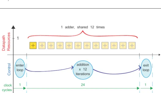
Usually, the repetitive operations described by the loop are realized by a single piece of hardware implementing the body of the loop. To take a simple

(30)

illustrative example, if a loop was designed to add the individual elements of two, 12 element arrays, then conceptually the implementation would in-volve a single adder (the body of the loop), shared 12 times according to the number of loop iterations.There is some latency associated with each iteration of the loop, and in this case, the latency is affected by interactions with the memory interfaces at the inputs and output of the function.

Additional clock cycles are also required for entering and exiting the loop. Code for this example is provided in 2.1. Analysis of HLS synthesis with default settings shows that the overall latency is 26 clock cycles: 2 cycles each for 12 iterations (including reading the inputs from memory, adding, and writing the output to memory), and a further two clock cycles for entering and exiting the loop. Execution is illustrated in Figure 2.1.

Listing 2.1: Example code for a loop adding the elements of two arrays

void add_array (short c[12], short a[12], short b[12]) { short j; // loop variable add_loop: for (j=0;j<12;j++) { c[j] = a[j] + b[j]; } }

Figure 2.1: Extraction of addition loop into datapath and control logichow transforma-tions affect the hardware implementation.

2.2.1 Simple Loop Architecture Variations

The default, rolled loop implementation may not always be desirable, but there are alternatives for implementing a loop

(31)

• Unrolled: In a rolled implementation, a single instance of the hard-ware is inferred from the loop body and shared to the maximum extent. Unrolling a loop means that instead the hardware inferred from the loop body is created up to N times, where N is the number of loop iterations. In practice, the number of instances may be lower than N if other limiting factors are identified in the design, such as memory operations. The clear disadvantage of the unrolled version is that it consumes much larger area on the device than the rolled design, but the advantage is increased throughput.

• Partially unrolled This constitutes a compromise between rolled and unrolled and is typically used when a rolled implementation does not provide high enough throughput. If a rolled architecture represents minimal hardware cost but maximal time sharing (lowest through-put), and an unrolled architecture represents maximal hardware cost but minimal sharing (highest throughput), then we may try to find a different balance between the two. Control is exerted by the use of directives, and a number of different positions in the trade-off may be possible.

With reference to the upper section of 2.1, which depicts a rolled ar-chitecture, fully or partially unrolling the loop would cause the number of datapath resources (adders) to increase, but to be shared to a lesser extent. Meanwhile, in the lower section of the diagram, the large, central state con-stituting the addition of array elements would require fewer clock cycles to complete. When fully unrolled, the implementation effectively does not con-tain a loop, and as a result, the loop entry and exit clock cycles are saved, too.

With these observations in mind, the decision to select a rolled, unrolled, or partially unrolled implementation for the loop will be based on the specific requirements of the application, particularly in terms of the target through-put and any constraint on area utilization that may apply.

2.2.2 Optimization: Merging Loops

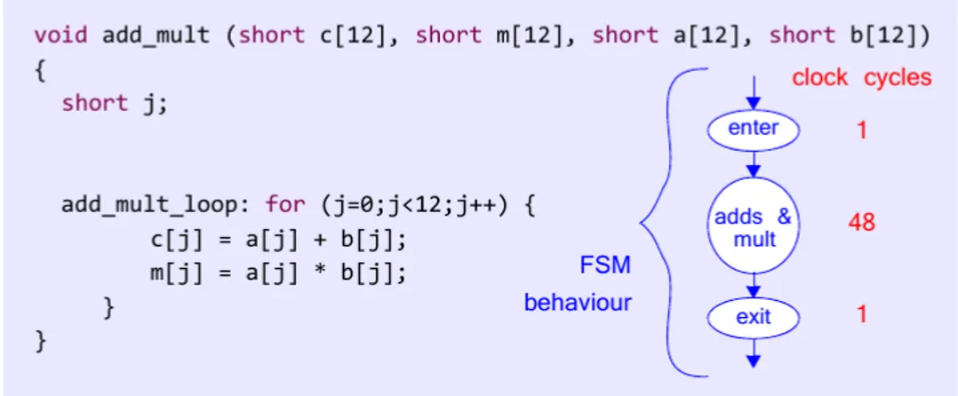
In some cases, there might be two loops occurring one after the other in the code. For instance, the addition loop in the example of 2.1 might be followed by a similar loop which multiplies the elements of the two arrays. Assuming that the loops are both rolled (according to the default mode), a possible optimization, in this case, would be to merge the two loops, such that there is only one loop, with both the addition and multiplication operations being conducted within the single loop body.

The advantage of merging loops may not be immediately obvious, but in fact, it relates to the control aspect of the design. Control is realized in the form of a Finite State Machine (FSM), with each loop corresponding

(32)

Figure 2.2: Consecutive loops for addition and multiplication within a function

to at least one state; thus the FSM can be simplified due to the merging of loops, as this results in fewer loops overall, and thus fewer FSM states. This is demonstrated by the code examples in Figures 2.2 and 2.3. The first example shows two separate loops, one each for addition and multiplication of the arrays, while the second shows the effect of merging the loops to create a single loop.

The add loop represents 12 iterations of an addition operation (which takes 2 clock cycles), while the mult loop represents 12 iterations of a mul-tiplication operation (which takes 4 clock cycles). Therefore, the overall latencies of the two loops are 24 and 48 clock cycles, respectively. Merging the loops has the effect that the latency of the new, combined loop reduces the length of the original two loops, i.e. 48 clock cycles. One further clock cycle is saved due to the removed loop transition, i.e. the ’exit/enter’ state in Figure 2.2.

2.2.3 Nested Loops

Another common configuration is to nest loops, i.e., place one loop inside another. There may even be multiple levels of nesting. To give an example of a 2-level nested loop, suppose we extend our array addition example from linear arrays to 2-dimensional arrays. Mathematically, this is equivalent to adding two matrices, as shown in 2.1.

  f00 f01 f02 f03 f10 f11 f12 f13 f20 f21 f22 f23  =   d00 d01 d02 d03 d10 d11 d12 d13 d20 d21 d22 d23  +   e00 e01 e02 e03 e10 e11 e12 e13 e20 e21 e22 e23   (2.1) 13

(33)

Figure 2.3: Merged addition and multiplication loops

Figure 2.4: Example code for nested loops adding the elements of two dimensional arrays

Now, in order to add the arrays, we must iterate through the rows, and for each row, iterate through the columns, adding together the two values for each array element. Coding the matrix addition operation requires an outer and an inner loop to cycle through the rows and columns, respectively, as shown by the code example in 2.4. According to 2.1, there are 3 rows and 4 columns, and this determines the limits of the nested loops (note that indexing starts as zero, as per the usual convention). Extending this idea, it would be possible to work with three dimensional arrays, or even higher dimensions, by increasing the levels of nesting in the loop structure.

2.2.4 Optimization: Flattening Loops

In the case of nested loops, there is an option to perform ’flattening’. This means that the loop hierarchy is effectively removed during high-level syn-thesis while preserving the algorithm, i.e. all of the operations performed

(34)

by the loop(s). The advantage of flattening is similar to merging: the ad-ditional clock cycles associated with transitioning into or out of a loop are avoided, meaning that the overall duration of algorithm execution reduces, thus improving the achievable throughput.

In order to explain flattening in further detail, it is necessary to clarify the terms loop and loop body. By loop, we refer to an entire code structure of a set of statements repeated a defined number of times. The statements inside the loop, i.e. the statements that are repeated, are the loop body. For instance, column loop is a loop, and the statements contained within column loop correspond to the loop body.

When loops are nested, and again taking the example of a 2-level nested structure, the outer loop body contains another loop, i.e. the inner loop. The outer loop body (including the inner loop) is executed a certain number of times; for instance, row loop has 3 repetitions in the example of Figure 2.4, and hence there are 3 executions of the inner loop, column loop. Each execution of the inner loop involves repeating the inner loop body a specified number of times, as well: in our example, a statement to calculate the matrix element f [j][k] is executed 4 times, where j is the row index and k is the column index.

The overhead of loop transitioning means that two additional clock cycles are required each time the inner loop is executed, i.e. one to enter the inner loop, and one to exit from it.

To clarify this point, a diagram depicting the control flow for our ma-trix addition example, and associated clock cycles, is provided in 2.5. This represents the original loop structure. The process of flattening ’unrolls’ the inner loop, and as a consequence, reduces the number of clock cycles asso-ciated with transitioning into and out of loops; specifically, the ’enter inner’ and ’exit inner’ states in 2.5 are removed. These would have been repeated 3 times, hence 6 clock cycles are saved in total in this case.

In our simple 3 × 4 matrix addition example, the saving equates to 6 clock cycles, but in other examples, this could be considerably higher (in particular where the outer loop iterates many times, or there are several layers of nesting), and thus there is a clear motivation to flatten loops. Similar to merging of loops, flattening can be achieved by a directive and does not involve explicit unrolling of the loop by manually changing the code. However, depending on its initial form, some manual restructuring may also be required in order to achieve a loop structure optimal for flattening.

2.2.5 Pipelining Loops

The direct interpretation of a loop written in C code is that executions of the loop occur consecutively, i.e. each loop iteration cannot begin until the previous one has completed. In hardware terms, this translates to a single set of hardware (as inferred from the loop body) that is capable of executing

(35)

Figure 2.5: Control flow through the matrix addition, without flattening (clock cycles in circles)

the operations of only one loop iteration at any particular instant, and which is shared over time according to the number of loop iterations. Throughput is limited when a set of operations are grouped together into a processing stage. In the case of loops, the loop body (i.e. the set of repeated operations) forms such a stage, and without pipelining, this would result in all stages operating in a sequential manner, and within them, all operations executing in a sequential manner. In effect, all operations from all iterations of the loop body would occur one after the other. The total number of clock cycles to complete the execution of a loop, N loop, would therefore be:

Nloop= (J × Nbody) + Ncontrol (2.2)

where J is the number of loop iterations, N+body is the number of clock cycles to execute all operations in the loop body, and N control represents the overhead of transitioning into and out of the loop.

The insertion of pipelining into the loop means that registers separate the implemented operators within the loop body. Given that the loop body is repeated several times, this carries the implication that operations within loop iteration j + 1 can commence before those of the loop iteration j have completed. In fact, at any instant, operations corresponding to several dif-ferent iterations of the loop may be active.

As a consequence of pipelining the loop, the hardware required to imple-ment the loop body is more fully utilized, and loop performance is improved in terms of both throughput and latency. The effect of adding a pipelining directive can, therefore, be considerable, especially where there are multiple

(36)

operations within the loop body, and many iterations of the loop are per-formed. When working with nested loops, it is useful to consider at which level of hierarchy pipelining should be applied. Pipelining at a certain level of the hierarchy will cause all levels below (i.e. all nested loops) to be unrolled, which may produce a more costly implementation than intended. There-fore, a good balance between performance and resource utilization may be achieved by pipelining only at the level of the innermost loop (for instance, column loop in Figure 2.5).

For more information about theoretical and mathematical fundamentals of loop transformations, based on the polyhedral model, refer to Appendix B.

2.3 External Tools and Frameworks

2.3.1 Profiling Tools

As indicated in chapter 4, to find the critical section of the code which is considered as computational or memory intensive should be identified before applying any optimizations. it is crucial to tune, transform and modify the section of the code which impacts critically on computations, CPU inter-rupts, and memory accesses.

Throughout this research different profiling tools got tested to obtain required performance metrics. Amongst them three candidates were Perf, GProf and Valgrind. As Perf and GProf were unable to measure perfor-mance metrics for small programs and also due to compatibility problems, we selected Valgrind as the main profiling tool in the framework. We also wrote three scripts to automate profiling via different tools. To pinpoint the critical section of the code, three execution features are taken into ac-count, the execution time of a particular function,the number of the times a function is called and (Execution time × #f unction call). Alongside these performance measurements, we also investigate call graphs, generated by Callgrind to decide about the hot function of the code.

Framework’s high-level Profiler

Kcachegrind is the highest level profiler integrated into the framework which is actually a profile data visualization. Callgrind uses runtime instrumen-tation via the Valgrind framework for its cache simulation and call-graph generation. This way even shared libraries and dynamically opened plug-ins can be profiled. The data files generated by Callgrind can be loaded into Kcachegrind for browsing the performance results. All experiments and benchmarks in this thesis are profiled by Kcachegrind. For each code the above-mentioned performance measurements were captured, meaning that we had at most three candidates function to apply software

(37)

tions, code transformation and hardware accelerator selection for HW/SW designs(Co-designs).

“In software engineering, profiling (”program profiling”, ”software profiling”) is a form of dynamic program analysis that measures, for example, the space (memory) or time complexity of a program, the usage of particular instruc-tions, or the frequency and duration of function calls. Most commonly, pro-filing information serves to aid program optimization”

2.3.2 Orio

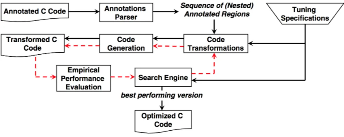
Orio [10] is an empirical performance-tuning system that takes annotated C source code as input, generates many optimized code variants of the an-notated code, and empirically evaluates the performance of the generated codes, ultimately selecting the best-performing version to use for production runs. Orio also supports automated validation by comparing the numerical results of the multiple transformed versions.

The Orio annotation approach differs from existing annotation- and compiler-based systems in the following significant ways. First, through de-signing an extensible annotation parsing architecture, it is not committing to a single general-purpose language. Thus, Orio can define annotation gram-mars that restrict the original syntax, enabling more effective performance transformations (e.g., disallowing pointer arithmetic in a C-like annotation language); furthermore, it enables the definition of new high-level languages that retain domain-specific information normally lost in low-level C or For-tran implementations. This feature, in turn, expands the range of possible performance-improving transformations.

Figure 2.6: Overview of Orio’s code generation and empirical tuning process.

Second, Orio was conceived and designed with the following requirements in mind: portability (which precludes extensive dependencies on external packages), extensibility (new functionality must require little or no change

(38)

to the existing Orio implementation, and interfaces that enable integration with other source transformation tools must be defined), and automation (ultimately Orio should provide tools that manage all the steps of the per-formance tuning process, automating each step as much as possible). Third, Orio is usable in real scientific applications without requiring reimplemen-tation. This ensures that the significant investment in the development of complex scientific codes is leveraged to the greatest extent possible.

Figure 2.6 shows a high-level graphical depiction of the code generation and tuning process implemented in Orio. Orio can be used to improve per-formance by source-to-source transformations such as loop unrolling, loop tiling, and loop permutation. The input to Orio is C code containing struc-tured comments that include a simplified expression of the computation, as well as various performance-tuning directives. Orio scans the marked-up input code and extracts all annotation regions. Each annotation region is then processed by transformation modules. The code generator produces the final C code with various optimizations that correspond to the specified annotations. Unlike compiler approaches, we do not implement a full-blown C compiler; rather, we use a pre-compiler that parses only the language-independent annotations.

Figure 2.7: Integration of Pluto and Orio

Orio can also be used as an automatic performance-tuning tool. The code transformation modules and code generator produce an optimized code ver-sion for each distinct combination of performance parameter values. Then each optimized code version is executed and its performance evaluated. Af-ter iAf-teratively evaluating all code variants, the best-performing code is picked as the final output of Orio. Because the search space of all possible opti-mized code versions can be huge, a brute-force search strategy is not always feasible. Hence, Orio provides various search heuristics for reducing the size of the search space and thus the empirical testing time.

(39)

A number of source-to-source transformation tools for performance opti-mization exist. Using these tools to achieve (near) optimal performance on different architectures, however, is still a nontrivial task that requires sig-nificant architectural and compiler expertise. Orio has been extended with an external transformation program, called Pluto [11]. This integration also demonstrates the easy extensibility of Orio and the ability to leverage other source transformation approaches.

Pluto is a source-to-source automatic transformation tool aimed at op-timizing a sequence of nested loops for data locality and coarse-grained par-allelism simultaneously. Pluto employs a polyhedral model of arbitrary loop nests, where the dynamic instance (iteration) of each statement is viewed as an integer point in a well-defined space called the statement’s polyhedron.

This statement representation and a precise characterization of data de-pendencies enable Pluto to construct mathematically correct complex loop transformations. Pluto’s polyhedral-based transformations result in im-proved cache locality and loops parallelized for multi-core architecture. Fig-ure 2.7 outlines the overall structFig-ure of the Pluto-Orio integrated system, which is implemented as a new optimization module in Orio.

2.3.3 OpenTuner

OpenTuner [12] is a framework for building domain-specific program au-totuners. OpenTuner features an extensible configuration and technique representation able to support complex and user-defined data types and custom search heuristics. It contains a library of predefined data types and search techniques to make it easy to setup a new project. Thus, OpenTuner solves the custom configuration problem by providing not only a library of data types that will be sufficient for most projects, but also extensible data types that can be used to support more complex domain specific represen-tations when needed. A core concept in OpenTuner is the use of ensembles of search techniques. Figure 2.8 illustrates the structure of OpenTuner.

Many search techniques (both built-in and user-defined) are run at the same time, each testing candidate configurations. Techniques which perform well by finding better configurations are allocated larger budgets of tests to run, while techniques which perform poorly are allocated fewer tests or disabled entirely. Techniques are able to share results using a common results database to constructively help each other in finding an optimal solution.

Algorithms add results from other techniques as new members of their population. To allocate tests between techniques we use an optimal solution to the multi-armed bandit problem using the area under the curve credit assignment. Ensembles of techniques solve the large and complex search space problem by providing both robust solutions to many types of large search spaces and a way to seamlessly incorporate domain-specific search

(40)

Figure 2.8: OpenTuner structure

techniques.

Figure 2.9: OpenTuner components

Figure 2.9 provides an overview of the major components in OpenTuner. The search process includes techniques, which use the user-defined configu-ration manipulator in order to read and write configuconfigu-rations. The measure-ment processes evaluate candidate configurations using a user-defined mea-surement function. These two components communicate exclusively through a results database used to record all results collected during the tuning pro-cess, as well as providing the ability to perform multiple measurements in parallel.

(41)

OpenTuner and HLS

As already mentioned in methodology description, the two-step code mod-ifications impact positively on different design methodologies. Application auto-tuning increase the multiplication block size which makes the corre-sponding synthesized hardware make use of LEs more efficiently. Depending on the type of FPGA this size approaches to an optimum value which makes the multiplication outperform both in HW and SW.

It is important to understand the differences between Orio and Open-Tuner. Orio is a source to source compiler which also reports some opti-mum compiler flags. But OpenTuner use application parameter tuning, it can tune some algorithmic parameters embedded inside the code and it is independent of the source to source compilation flow.

2.3.4 LegUp

LegUp [13] is an open-source high-level synthesis (HLS) tool that accepts a C program as input and automatically synthesizes it into a hybrid system. The hybrid system comprises an embedded processor and custom accel-erators that realize user-designated compute-intensive parts of the program with improved throughput and energy efficiency.Embedded system designers can achieve energy and performance benefits by using dedicated hardware accelerators.

However, implementing custom hardware accelerators for an application can be difficult and time intensive. LegUp is an open-source high-level syn-thesis framework that simplifies the hardware accelerator design process. With LegUp, a designer can start from an embedded application running on a processor and incrementally migrate portions of the program to hardware accelerators implemented on an FPGA. The final application then executes on an automatically-generated software/hardware co-processor system.

LegUp includes a soft processor because not all program segments are appropriate for hardware implementation. Inherently sequential computa-tions are well-suited for software (e.g. traversing a linked list); whereas, other computations are ideally suited for hardware (e.g. addition of integer arrays). Incorporating a processor also offers the advantage of increased high-level language coverage.

Program segments that use restricted C language constructs can execute on the processor (e.g. recursion). LegUp is written in modular C++ to permit easy experimentation with new HLS algorithms. It leverages the state-of-the-art LLVM (low-level virtual machine) compiler framework for high-level language parsing and its standard compiler optimizations [14].

(42)

LegUp Design flow

The LegUp design flow comprises first compiling and running a program on a standard processor, profiling its execution, selecting program segments to target to hardware, and then re-compiling the program to a hybrid hard-ware/software system.

Figure 2.10 illustrates the detailed flow. Referring to the labels in the fig-ure, at step 1, the user compiles a standard C program to a binary executable using the LLVM compiler. At 2, the executable is run on an FPGA-based MIPS processor. It makes use of Tiger MIPS processor from the Univer-sity of Cambridge [UniverUniver-sity of Cambridge 2010], but it is also possible to migrate to other processors such as ARM core.

The MIPS processor has been augmented with extra circuitry to profile its own execution. Using its profiling ability, the processor is able to identify sections of program code that would benefit from hardware implementation, improving program throughput and power. Specifically, the profiling results drive the selection of program code segments to be re-targeted to custom hardware from the C source. Having chosen program segments to target custom hardware, at step 3 LegUp is invoked to compile these segments to synthesizable Verilog RTL.

Presently, LegUp HLS operates at the function level: entire functions are synthesized to hardware from the C source. Moreover, if a hardware function calls other functions, such called functions are also synthesized to hardware. In other words, we do not allow a hardware-accelerated function to call a software function. The RTL produced by LegUp is synthesized to an FPGA implementation using standard commercial tools at step 4. As illustrated in the figure, LegUp’s hardware synthesis and software compilation are part of the same LLVM-based compiler framework.

In step 5, the C source is modified such that the functions implemented as hardware accelerators are replaced by wrapper functions that call the accelerators (instead of doing computations in software). This new modified source is compiled to a MIPS binary executable. Finally, in step 6 the hybrid processor/accelerator system executes on the FPGA.

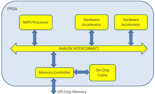
Figure 2.11 elaborates on the target system architecture. The processor connects to one or more custom hardware accelerators through a standard on-chip interface. As our initial hardware platform is based on Cyclone II FPGA, the Altera Avalon interface for processor/accelerator communication is used. A shared memory architecture is used, with the processor and ac-celerators sharing an on FPGA data cache and off-chip main memory. The on-chip cache memory is implemented using block RAMs within the FPGA fabric (M4K blocks on Cyclone II). Access to memory is handled by a mem-ory controller. The architecture in Figure 2.11 allows processor/accelerator communication across the Avalon interface or through memory.

(43)

Figure 2.10: LegUp Design Flow

(44)

LegUp High-Level Hardware Synthesis

High-level synthesis has traditionally been divided into three steps: • allocation

• scheduling • binding

Allocation determines the amount of hardware available for use (e.g., the number of adder functional units), and also manages other hardware con-straints (e.g., speed, area, and power). Scheduling assigns each operation in the program being synthesized to a particular clock cycle (state) and generates a finite state machine.

Binding assigns an application operation to specific hardware units. The decisions made by binding may imply sharing functional units between op-erations, and share registers/memories between variables. All the above-mentioned stages are integrated into LegUp procedures.

The LegUp open-source HLS tool is implemented within the LLVM com-piler framework, which is used in both industry and academia. LLVM’s front-end, clang, parses the input C source and translates it into LLVM’s intermediate representation (IR). The IR is essentially machine-independent assembly code in static-single assignment (SSA) form, composed of simple computational instructions (e.g., add, shift, multiply) and control-flow in-structions (e.g., branch). LLVM’s opt tool performs a sequence of compiler optimization passes on the program’s IR, each such pass directly manipu-lates the IR, accepting an IR as input and producing a new/optimized IR as output.

A high-level diagram of the LegUp Hardware synthesis flow is shown in Figure 2.12. The LegUp HLS tool is implemented as back-end passes of LLVM that are invoked after the standard compiler passes. LegUp accepts a program’s optimized IR as input and goes through the four stages shown in Figure 2.12 (1) Allocation, (2) Scheduling, (3) Binding, and (4) RTL generation) to produce a circuit in the form of synthesizable Verilog HDL code.

The allocation stage allows the user to provide constraints to the HLS algorithms, as well as data that characterizes the target hardware. Examples of constraints are limits on the number of hardware units of a given type that may be used, the target circuit critical path delay, and directives pertaining to loop pipelining and resource sharing. The hardware characterization data specifies the speed (critical path delay) and area estimates (number of FPGA logic elements) for each hardware operator (e.g., adder, multiplier) for each supported bandwidth (typically 8, 16, 32, and 64 bit). The characterization data is collected only once for each FPGA target family using automated

(45)

Figure 2.12: Design flow with legup

scripts. The scripts synthesize each operation in isolation for the target FPGA family to determine their speed and area.

At the scheduling stage, each operation in the program (in the LLVM IR) is assigned to a particular clock cycle (state) and an FSM is generated. The LegUp scheduler, based on the SDC formulation, operates at the basic block level, exploiting the available parallelism between instructions in a basic block. A basic block is a sequence of instructions that has a single entry and exit point.

The scheduler performs operation chaining between dependent combina-tional operations when the combined path delay does not exceed the clock period constraint-chaining refers to the scheduling of dependent operations into a single clock cycle. Chaining can reduce hardware latency (number of cycles for execution) and save registers without impacting the final clock period.

The binding stage assigns operations in the program to specific hardware units. When multiple operators are assigned to the same hardware unit, multiplexers are generated to facilitate the sharing. Multiplexers require a significant amount of area when implemented in an FPGA logic fabric.

Consequently, there is no advantage to sharing all but the largest func-tional units, namely multipliers, dividers, and recurring patterns of smaller operators. Multiplexers also contribute to circuit delay, and thus they are used judiciously by the HLS algorithms. LegUp also recognizes cases where there are shared inputs between operations, which allows hardware units to be shared without creating multiplexers. Last, if two operations with non-overlapping lifetime intervals are bound to the same functional unit, then a

(46)

single output register is used for both operations. This optimization saves a register as well as a multiplexer.

The RTL generation stage produces synthesizable Verilog HDL regis-ter transfer level code. One Verilog module is generated for each function in the C source program. Results show that LegUp produces solutions of comparable quality to a commercial

2.4 Target Architectures

MIPS architecture is the main target that we followed due to the compatibil-ity of the Orio and LegUp with the architecture and also, using the common reference architecture in computer science.

2.4.1 MIPS

As the MIPS processor is part of the framework to implement software exe-cution and also code tuning is applied based on this architecture, we roughly illustrate the processor organization. Figure 2.13 shows the datapath fellow with the control unit of MIPS architecture. The key concepts of the original MIPS architecture are:

• Five-stage execution pipeline: fetch, decode, execute, memory-access, write-result

• Regular instruction set, all instructions are 32-bit • Three-operand arithmetical and logical instructions • 32 general-purpose registers of 32-bits each

• No status register or instruction side-effects

• No complex instructions (like stack management, string operations, etc.)

• Optional coprocessors for system management and floating-point • Only the load and store instruction access memory

• Flat address space of 4 GBytes of main memory (23_{2 bytes)}

• Memory-management unit (MMU) maps virtual to actual physical addresses

• Optimizing C compiler replaces hand-written assembly code • Hardware structure does not check dependencies - not ”foolproof”

(47)

• But software toolchain knows about hardware and generates correct code

Figure 2.13: MIPS datapath with control unit.

One of the key features of the MIPS architecture is the regular register set. It consists of the 32-bit wide program counter (PC), and a bank of 32 general-purpose registers called r0..r31, each of which is 32-bit wide. All general-purpose registers can be used as the target registers and data sources for all logical, arithmetical, memory access, and control-flow instructions. Only r0 is special because it is internally hardwired to zero. Reading r0

(48)

always returns the value 0x00000000, and a value written to r0 is ignored and lost.

Note that the MIPS architecture has no separate status register. Instead, the conditional jump instructions test the contents of the general-purpose registers, and error conditions are handled by the interrupt/trap mechanism. Two separate 32-bit registers called HI and LO are provided with the integer multiplication and division instructions.

2.4.2 Emulation Environments

The proposed methodology needs a MIPS/ARM processor to optimize ar-chitectural dependent parameters and to find the best-transformed version of the code which outperforms among others. To find a versatile and appli-cable clue, we considered several approaches including using an actual MIP-S/ARM processor, Open Virtual Platform(OVP), and QEMU. To tackle compatibility issues with other elements of the framework such as Orio and OpenTuner, and also the potential to access the emulator remotely using a virtual private network and a secure shell, QEMU was chosen to emulate our MIPS environment. In case of ARM platform, we used our DE1-SoC development board which provides an embedded arm processor (Hard-core) on a Cyclon V FPGA.

QEMU is a generic and open source machine emulator and virtualizer. When used as a machine emulator, QEMU can run OSes and programs made for one machine (e.g. an ARM board) on a different machine (e.g. your own PC). By using dynamic translation, it achieves very good performance.

When used as a virtualizer, QEMU achieves near native performance by executing the guest code directly on the host CPU. QEMU supports virtualization when executing under the Xen hypervisor or using the KVM kernel module in Linux. When using KVM, QEMU can virtualize x86, server and embedded PowerPC, 64-bit POWER, S390, 32-bit and 64-bit ARM, and MIPS guests.

2.4.3 Development Board

At the end of compilation and synthesis process, binary and SRAM object files are downloaded on an FPGA. we used DE1-SoC evaluation board to implement the designs. Figure 2.14 shows the structure of the board. Figure 2.15 shows the architecture of Cyclon V which consist of the logic part, namely FPGA, and a hard Processing System called HPS which is actually an ARM core.

(49)

(50)

Figure 2.15: Altera’s Cyclon V SoC Architecture

(51)

(52)

Chapter 3

State of the Art

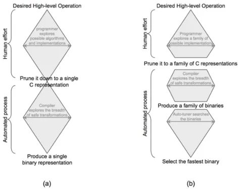
Automatic Performance Tuning or ”Auto-tuning”, is an empirical, feedback-driven performance optimization technique designed to maximize perfor-mance across a wide variety of architectures without sacrificing portabil-ity or productivportabil-ity. Over the years, autotuning has expanded from sim-ple loop tiling and unroll-and-jam to encompass transformations to data structures, parallelization, and algorithmic parameters. Automated tun-ing or autotuntun-ing has become a commonly accepted technique used to find the best implementation for a given kernel on a given single-core machine [15, 16, 17, 18, 19]. Figure 3.1 compares the traditional and autotuning ap-proaches to programming. 3.1(a) shows the common Alberto Sangiovanni-Vincentelli (ASV) triangle [20]. A programmer starts with a high-level op-eration or kernel he wishes to implement. There is a large design space of possible implementations that all deliver the same functionality.

However, he prunes them to a single C program representation. In do-ing so, all high-level knowledge is withheld from the compiler which in turn takes the C representation and explores a variety of safe transformations given the little knowledge available to it. The result is a single binary rep-resentation. Figure 3.1(b) presents the autotuning approach. The program-mer implements an autotuner that rather than generating a single C-level representation, generates hundreds or thousands. The hope is that in gen-erating these variants some high-level knowledge is retained when the set is examined collectively. The compiler then individually optimizes these C kernels producing hundreds or machine language representations.

The autotuner then explores these binaries in the context of the actual data set and machine. There are three major concepts with respect to au-totuning: the optimization space, code generation, and exploration. First, a large optimization space is enumerated. Then, a code generator produces C code for those optimized kernels. Finally, the autotuner proper explores the optimization space by benchmarking some or all of the generated kernels searching for the best performing implementation. The resultant

(53)

configura-Figure 3.1: ASV triangles for the conventional and auto-tuned approaches to program-ming.