FACOLT `A DI SCIENZE MATEMATICHE, FISICHE E NATURALI Corso di Laurea Magistrale in Matematica
REPRESENTATIONS
OF SYMMETRIC GROUPS
ON THE HOMOLOGY OF DUAL
MATROIDS OF COMPLETE GRAPHS
Tesi di Laurea in Topologia Algebrica
Relatore:
Chiar.mo Prof.
Luca Moci
Presentata da:
Gian Marco Pezzoli
Correlatore:
Chiar.ma Prof.ssa
Nicoletta Cantarini
VI Sessione
This thesis investigates the representations of the symmetric group on the homology of the dual matroid of a complete graph. These representations arise as follows: with each graph we can associate a matroid, by taking the set of edges of the graph as ground set and the edge sets of simple cycles as the circuits of the matroid. We focus on the dual of the matroid of the complete graph Kn, which coincides with the dual matroid of the independent sets of
the root system of type An 1. We calculate the homology of the simplicial
complex L associated with this matroid.
Permuting the vertices of the complete graph induces a permutation on the edge set which is a vertex map of the simplicial complex. This vertex map sends independents to independents, thus inducing a simplicial map from the polytope of L to itself, hence on the homology spaces of L. This defines a representation of the symmetric group Sn on the homology Hi(L,C), which
turns out in this case to be non trivial if i = (n2 3n)/2. We show that the
above representation is induced from a primitive representation of Cn, the
cyclic subgroup of order n.
This problem has been suggested by the study of the Cattani-Kaplan-Schmid complex relative to a family of completely reducible spectral curves for the Hitchin fibration of type An, performed by de Cataldo, Heinloth and
Migliorini ([7]). The dual graph of a spectral such curve is the complete graph, and the action of the symmetric group on the irreducible components of the curve yields an action on the vertices of the complete graph .
In chapter one we give some background regarding root systems and group i
representations. In the first section we focus on the root system of type A, whose Weyl group is the symmetric group. The action of the Weyl group Sn on the root system An 1, without considering the sign, will correspond
to the action of the symmetric group on the edges of the complete graph. In particular, in the second section, we define the induced representation and we compute an example that will be important for our purposes.
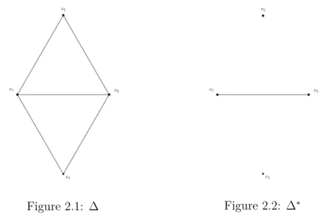
In chapter two we recall the necessary preliminaries regarding simplicial complexes, homology, and matroid theory. In the first section we prove Alexander duality, that will be crucial for the main result of this thesis. In the second section we see how the action on the ground set induces a simplicial map and furthermore a map on the homology. At the end of the chapter we describe the case of K4 (or equivalently +(A3)).
In chapter three, following Stanley [20], we compute the representations on the homology of the partition lattice ⇧nwith the action induced from the
permutations of 1, 2, . . . , n. We see that these representations are exactly the induced representations from Cn to Sn. At the end of the chapter we report
the explicit calculation of the representations of ⇧4. The reader can compare
this example with the one at the end of chapter 2.
The results obtained in these two examples are generalized in chapter four. In the first section, given any simple matroid M , we apply Alexander duality to the following two abstract simplicial complexes: the independence set of the dual matroid M⇤ and the nonspanning simplicial complex of M ,
i.e. the set of all subsets of the groundset which do not contain any basis of M . In the second section we use a result due to Folkman to show the isomorphism between the homology of the non spanning simplicial complex and the homology of its lattice of flats. Combining the last two results we prove that the homology of the dual matroid M⇤ is isomorphic to the
homology of the lattice of flats of M . On the other hand, the lattice of flats of the cycle matroid of Kn is exactly the partition lattice ⇧n. Since these
isomorphisms are natural, i.e. they do not depend on the choice of a basis, they are compatible with the action of Sn. Consequently the representations
we have studied in chapter three coincide with the representations we want to study in this thesis.
It would be interesting to extend what has been done in this thesis to any type of root system. In chapter five we compute the representations of the Weyl group on the homology of the dual matroid associated to the root system of type B2.
Introduction i 1 Preliminaries in Algebra 1
1.1 Root systems . . . 1
1.1.1 Basic definitions . . . 1
1.1.2 Root systems of type A . . . 3
1.2 Group representations . . . 7
1.2.1 Basic definitions . . . 7
1.2.2 Irreducible representations . . . 11
1.2.3 The character of a representation . . . 13
1.2.4 Decomposition of the regular representation . . . 17
1.2.5 Number of irreducible representations . . . 19
1.2.6 Abelian subgroups and the cyclic group Cn . . . 23
1.2.7 Induced representations . . . 24
2 Preliminaries in Topology and Combinatorics 35 2.1 Simplicial homology . . . 35
2.1.1 Simplicial complexes . . . 35
2.1.2 Abstract simplicial complex . . . 39
2.1.3 Homology groups . . . 40
2.1.4 Homology groups with arbitrary coefficients . . . 44
2.1.5 Cohomology groups . . . 46
2.1.6 Homomorphism induced by a simplicial map . . . 49
2.1.7 Alexander Duality . . . 50 v
2.2 Matroid theory . . . 58
2.2.1 Basic definitions . . . 58
2.2.2 Basis, Rank and Closure Operator . . . 62
2.2.3 Duality . . . 65
2.2.4 Lattice of flats . . . 66
2.2.5 Lattice of flats of the complete graph Kn . . . 68
2.2.6 Isomorphism between M ( +(A n 1), I) and M (Kn) . . 70
2.2.7 The Sn-action on the vertices of Kn . . . 72
3 Representations on the homology of the partition lattice 81 3.1 On the homology of a poset . . . 81
3.2 On the homology of the partition lattice ⇧n . . . 94
4 Representations on the homology of dual matroid of com-plete graphs 105 4.1 Alexander duality for non spanning matroid and independence dual matroid . . . 105
4.2 Isomorphism between homology of non spanning complex of a matroid and homology of its lattice of flats . . . 107
4.3 Representations on the homology of dual matroid of a com-plete graph . . . 110 5 Representations on the homology for the root system B2 113
Preliminaries in Algebra
1.1
Root systems
In this Section we recall the fundamental notions of root system and we explicitly construct the root systems of type A that will be fundamental for this thesis.
1.1.1
Basic definitions
Let E be a finite-dimensional real vector space endowed with a positive definite symmetric bilinear form (·, ·).
Given a non-zero vector ↵2 E, let
P↵={v 2 E | (v, ↵) = 0}
be the hyperplane orthogonal to ↵, and let
↵ : E ! E
be an invertible linear transformation such that
↵(v) = v 8v 2 P↵, ↵(↵) = ↵.
It is sufficient to define ↵ on P↵ and ↵, since E = < ↵ > P↵.
It is easy to write down an explicit formula:
↵( ) =
2( , ↵) (↵, ↵) ↵
We defineh , ↵i = 2( ,↵)(↵,↵); notice thath , ↵i is linear only in the first variable. Definition 1.1. A subset of E is called a root system in E if the following axioms are satisfied:
(R1) is finite, 0 /2 , spans E (R2) If ↵2 , then c↵ 2 , c = ±1 (R3) 8 ↵, 2 ↵( ) = h , ↵i↵ 2
(R4) 8 ↵, 2 h , ↵i 2 Z
The elements of are called roots. The dimension of E, dimRE = l, is called the rank of the root system.
The following statements give the first indication that the axioms for root systems are quite restrictive.
Let ↵, 2 with 6= ±↵. Then:
a) (↵, ) =k↵kk k cos c↵ =) h↵, i = 2(↵, )( , ) = 2k kk↵kcos c↵ b) h↵, i = 0 () (↵, ) = 0
c) h↵, i and h , ↵i are always concordant. d) k↵k k k =) | h↵, i | | h , ↵i |
e) h↵, i h , ↵i = 4 cos2↵c 3 =) h↵, i h , ↵i 2 {0, 1, 2, 3}
Definition 1.2. A subset of is called a base if: (B1) is a base of E.
(B2) Each root 2 can be written as =P 2 n with integral coeffi-cients n all nonnegative or all nonpositive.
The roots in are called simple. If all n 0, we call positive and write 0; if all n 0, we call negative and write 0.
The collections of positive and negative roots (relative to ) will usually just be denoted by + and .
Definition 1.3. The root system is called irreducible if it cannot be par-titioned into the union of two proper subsets such that each root in one set is orthogonal to each root in the other.
Definition 1.4. Let be a root system in E. Denote by W the subgroup of GL(E) generated by the reflections ↵ with ↵2 . W is called the Weyl
group of .
By (R3) W permutes the elements of , so we can identify W with a subgroup of the symmetric group on , in particular W is finite.
1.1.2
Root systems of type A
Let E be the n-dimensional subspace of Rn+1 orthogonal to the vector
e1+· · · + en+1: E = x2 Rn+1| (x, e 1+· · · + en+1) = 0 Let also I =n n+1 X i=1 aiei | ai 2 Z o and I0 = I \ E Let be the set of all vectors ↵2 I0 such that (↵, ↵) = 2:
= ↵2 I0 | (↵, ↵) = 2 = ↵ 2 I0 | k↵k2 = 2 Let ↵2 ✓ E, we have for suitable ai 2 Z:
0 |{z} = ⇣ ↵, n+1 X j=1 ej ⌘ =⇣ n+1 X i=1 aiei, n+1 X j=1 ej ⌘ = a1+ . . . an+1 | {z }
Moreover k↵k2 = 2, 2 |{z} = ↵, ↵ = ⇣Xn+1 i=1 aiei, n+1 X i=1 aiei ⌘ = a2 1+ . . . a2n+1 | {z } For a fixed ↵2 , there must be two di↵erent ai, aj such that:
ai = 1 aj = 1 ak = 0, 8k 6= i, j
or
ai = 1 aj = 1 ak = 0, 8k 6= i, j
Every element of is of the form ei ej with i6= j:
= ei ej | i 6= j
is obviously finite and 0 /2 by definition. It is evident that spans E. Therefore (R1) is satisfied.
The choice of lengths we made make obvious that (R2) holds.
For (R3) it is enough to check that the reflection ↵with ↵2 sends to I0,
i.e ↵( )✓ I0, since then ↵( ) automatically consists of vectors of squared
lengths equal to two ( ↵ is an isometry, doesn’t change lengths). But then
(R3) follows directly from (R4):
↵( ) = h , ↵i↵ 2 I0, ↵2 I0
If (R4) holds, we have that h , ↵i 2 Z and then ↵( )2 .
Regarding (R4), let ↵, 2 ✓ I0 we have for suitable a
i, bi 2 Z: (↵, ) =⇣ n X i=1 aiei, n X j=1 bjej ⌘ = a1b1+· · · + anbn 2 Z It follows that h↵, i = 2(↵, ) (↵, ↵) = 2(↵, ) k↵k2 = (↵, )
Then h↵, i 2 Z. Therefore is a root system and is called the root system of type An.
The vectors ↵i = ei ei+1 (16 i 6 n) are linearly independent and for
i < j:
ei ej = (ei ei+1) + (ei+1 ei+2) +· · · + (ej 1+ ej)
The coefficients of the ↵i are all positive, so the ↵i form a base of .
= ↵i | 1 6 i 6 n
Finally, notice that the reflection ↵iwith respect to the root ↵i, permutes
the subscripts i, i + 1 and leaves all the others subscripts fixed.
↵i(↵i) = ↵i ↵i(↵i+1) = ↵i+1 h↵i+1, ↵ii↵i = ↵i+1+ ↵i
↵i(↵j) = ↵j h↵j, ↵ii↵i = ↵j 8j 6= i 1, i, i + 1
Thus ↵i corresponds to the transposition (i, i + 1) in the symmetric group
Sn+1. These transpositions generate Sn+1, so we obtain a natural
isomor-phism betweenW and Sn+1:
W ! Sn+1 ↵i 7 ! (i, i + 1)
If we think of An as embedded in Rn+1, the action of the Weyl group
cor-responds to a permutation of the coordinates of Rn+1. Each element of
W = Sn+1 induces a map on +
An in the following way: for each element
xi 2 +An consider the subspace Vi = Span{xi} of R
n+1.
Since W permutes the roots of An, it also permutes the Vi’s. By
iden-tifying the Vi with the xi we get a map on +An; in other words we consider
the action of the Weyl group on An without considering the sign.
Example 1. Let us consider the root system of type A3:
A3 ={±↵1,±↵2,±↵3,±(↵1+ ↵2),±(↵2+ ↵3),±(↵1+ ↵2+ ↵3)}
WA3 ! S4
↵1 7 ! (1, 2)
↵2 7 ! (2, 3)
If we consider 2 W, we call e the induced map on +An: ↵1 : A3 ! A3 ↵1 7 ! ↵1 ↵2 7 ! ↵1+ ↵2 ↵3 7 ! ↵3 e↵1 : + A3 ! + A3 ↵1 7 ! ↵1 ↵2 7 ! ↵1+ ↵2 ↵3 7 ! ↵3
For example, if f = ↵1 ↵3 then:
f : A3 ! A3 ↵1 7 ! ↵1 ↵2 7 ! ↵1+ ↵2+ ↵3 ↵3 7 ! ↵3 e f : +A3 ! + A3 ↵1 7 ! ↵1 ↵2 7 ! ↵1+ ↵2+ ↵3 ↵3 7 ! ↵3
1.2
Group representations
In this Section we recall the fundamental notions of the representations theory of finite groups. As an example, we focus on representations of the symmetric group, which is the most relevant for our purposes.
1.2.1
Basic definitions
Let V be a C-vector space and let GL(V ) be the group of isomorphisms of V onto itself. An element a2 GL(V ) is an invertible linear transformation of V . We will denote its inverse by a 1.
When V has a finite basis {e1, . . . , en}, each linear map:
a : V ! V
can be defined by a square matrix (aij) of order n. The coefficients aij are
complex numbers; they are obtained by expressing the images a(ej) as linear
combinations of the elements of the basis {e1, . . . , en}:
a(ej) = n
X
i=1
aijei
a is an isomorphism if and only if det(a) = det(aij)6= 0.
In this way the group GL(V ) can be identified with the group of invertible square matrices of order n.
Suppose now G is a finite group, with identity element 1 and with composi-tion:
G⇥ G ! G (s, t) 7 ! st
Definition 1.5. A linear representation of G in V is a group homomorphism ⇢ from the group G into the group GL(V ):
⇢ : G ! GL(V ) s 7 ! ⇢s
If V has finite dimension n, we say also that n is the degree of the represen-tation.
In other words, we associate each element s 2 G with an element ⇢s of
GL(V ) in such way that we have the following equality: ⇢st = ⇢(st) = ⇢(s)⇢(t) = ⇢s⇢t
Definition 1.6. Let ⇢ and ⇢0 be two representations of the same group G in
two vector spaces V and V0. These representations are said to be isomorphic
if there exists a linear isomorphism
⌧ : V ! V0
such that
⌧ ⇢(s) = ⇢0(s) ⌧ for all s2 G This is equivalent to say that the following diagram
V ⌧! V0 ⇢s ? ? y ? ? y⇢0 s V ⌧! V0
commutes for all s2 G.
When ⇢ and ⇢0 are given in matrix form by R
s and R0s respectively, this
means that there exists an invertible matrix T such that: T Rs= R0s T for all s2 G
Example 2. a) Let V be a vector space of dimension 1, then GL(V )' C⇤
whereC⇤denotes the multiplicative group of nonzero complex numbers. A representation of degree 1 of a group G is a homomorphism
⇢ : G ! C⇤
Since each element of G has finite order, the values ⇢(s) of ⇢ are roots of unity; in particular
|⇢(s)| = |⇢s| = 1
If we take ⇢(s) = 1 for all s2 G, we obtain a representation of G which is called the unit (or trivial ) representation.
b) Let g be the order of G, and let V be a vector space of dimension g, with a basis (et)t2G indexed by the elements t of G. For s 2 G, let ⇢s
be the linear map of V into V such that: ⇢s: V ! V
et 7 ! est
This defines a linear representation of G, which is called the regular representation of G. Its degree is equal to the order of G. Note that:
es= ⇢s(e1)
hence ⇢s(e1), s2 G form a basis of V .
Conversely, let W be a representation of G containing a vector w such that the elements ⇢s(w) with s 2 G, form a basis of W ; then W is
isomorphic to the regular representation under the following map: : Vreg ! W
es 7 ! ⇢s(w)
We recall the definition of K-algebra:
Definition 1.7. LetK be a field. A K-algebra is a K-vector space A equipped with an additional bilinear binary operation:
⇤ : A ⇥ A ! A (x, y) 7 ! x ⇤ y
A K-algebra is said to be associative if the product ⇤ is associative. An algebra is said to be unitary if it has an identity element with respect to the multiplication ⇤.
Definition 1.8. Let (A,⇤) and (A0, ?) be two K-algebras. A K-algebra
ho-momorphism is a linear map
: A ! A0
such that
Definition 1.9. Let A be an associative and unitaryK-algebra and let V be a vector space. A representation of A on V is a K-algebra homomorphism
e
⇢ : A ! End(V )
where End(V ) is the associative algebra of endomorphism of V .
Definition 1.10. Let ⇤ be a ring with unity 1⇤, an abelian group M is said
to be a left ⇤-module if there exists a map: f : ⇤⇥ M ! M such that: • f(1⇤, m) = m 8m 2 M • f( 1 2, m) = f ( 1, f ( 2, m)) 8m 2 M 8 1, 2 2 ⇤ • f( 1 + 2, m) = f ( 1, m) + f ( 2, m) 8m 2 M 8 1, 2 2 ⇤ • f( , m1+ m2) = f ( , m1) + f ( , m2) 8m1, m2 2 M 8 2 ⇤
We will often write . m instead of f ( , m).
Let be a representation of an associative and unitary algebra A : A ! End(V )
a 7 ! a
the vector space V can be seen as a left A-module through the action a . v = (a)(v) = a(v)
Definition 1.11. The group algebra K[G], where K is a field and G a group with operation⇤, is the set of all linear combinations of finitely many elements of G with coefficients in K, hence all elements of the form:
a1g1+ a2g2+· · · + angn ai 2 K, gi 2 G 8i = 1, . . . , n
This element can be denoted in general by X
g2G
agg
The group algebra K[G] is a K-algebra with respect to the addition de-fined by the following rule:
X g2G agg + X g2G bgg = X g2G (ag + bg) g;
the product by scalar is given by X g2G agg = X g2G ( ag) g
and the multiplication is the following X g2G agg ! X h2G bhh ! = X g,h2G (agbh) g⇤ h.
From this definition, it follows that the identity element of G is the unity of K[G].
Remark. Every linear representation of a group G on V ⇢ : G ! GL(V )
g 7 ! ⇢g
defines an algebra representation of K[G] on V in the following way: e
⇢ : K[G] ! End(V ) P
g2G gg 7 ! Pg2G g⇢g
Conversely, every algebra representation of K[G] on V defines a representa-tion of G on V by considering the restricrepresenta-tion of⇢ to the elements of G.e
1.2.2
Irreducible representations
Let ⇢ : G ! GL(V ) be a linear representation and let W be a vector subspace of V . Suppose that W is stable under the action of G, in other words suppose that for all x2 W , ⇢s(x)2 W for all s 2 G.
The restriction ⇢|Ws of ⇢s is then an isomorphism of W onto itself, and we
have:
Thus
⇢W : G ! GL(W )
s 7 ! ⇢|Ws
is a linear representation of G in W ; ⇢W is said to be a subrepresentation of
V .
Theorem 1.12. Let ⇢ : G ! GL(V ) be a linear representation of G in V and let W be a vector subspace of V stable under G. Then there exists a complement W0 of W which is stable under G. In other words, there exists
a subspace W0 such that:
i) V = W W0
ii) W0 is stable under the action of G
Proof . See [19], Theorem 1; pag 6.
Definition 1.13. Let ⇢ : G ! GL(V ) be a linear representation of G in V . We say that it is irreducible if V is not 0 and if no vector subspace of V is stable under G, except 0 and V .
By induction, Theorem 1.12 yields immediately the following:
Theorem 1.14. Every representation is a direct sum of irreducible repre-sentations.
Let V1 and V2 be two vector spaces. Let
⇢1 : G ! GL(V 1) s 7 ! ⇢1 s ⇢2 : G ! GL(V 2) s 7 ! ⇢2 s
be two linear representations of a group G. For s 2 G, define an element ⇢s 2 GL(V1⌦ V2) by the condition:
⇢s(x1 ⌦ x2) = ⇢1s(x1)⌦ ⇢2s(x2)
The existence and uniqueness of ⇢sfollows from the definition of tensor
prod-uct. We write:
We have thus defined a linear representation of G in V1⌦ V2:
⇢ : G ! GL(V1⌦ V2)
s 7 ! ⇢s= ⇢1s⌦ ⇢2s
which is called the tensor product of ⇢1 and ⇢2.
The tensor product of two irreducible representations is not in general irre-ducible.
1.2.3
The character of a representation
Let V be a vector space having a basis {e1, . . . , en}, and let a be a linear
map of V into itself, with associated matrix (aij). We recall that the trace
of a is the scalar Tr(a) = n X i=1 aii
It is the sum of the eigenvalues of a counted with their multiplicities, thus it does not depend on the choice of the basis.
Definition 1.15. Let ⇢ : G ! GL(V ) be a linear representation of a finite group G in the vector space V . For each s2 G, we set:
⇢(s) = Tr(⇢s)
The complex valued function
⇢: G ! C
s 7 ! Tr(⇢s)
is called the character of the representation ⇢. The following properties are straightforward:
Proposition 1.16. If is the character of a representation ⇢ of degree n, we have:
ii) (s 1) = (s) for s 2 G
iii) (tst 1) = (s) for s, t 2 G
Remark. A function
f : G ! C satisfying identity iii) is called a class function. Proposition 1.17. Let
⇢1 : G ! GL(V
1) ⇢2 : G ! GL(V2)
be two linear representations of a group G, and let 1 and 2 be their
char-acters. Then:
i) The character ⇢ of the direct sum representation
⇢ : G ! GL(V1 V2)
is equal to 1+ 2.
ii) The character ⇢ of the tensor product representation
⇢ : G ! GL(V1⌦ V2)
is equal to 1· 2.
Proof . See [19], Proposition 2; pag 11. Proposition 1.18 (Schur’s Lemma). Let
⇢1 : G ! GL(V
1) ⇢2 : G ! GL(V2)
be two irreducible representations of G, and let f be a linear mapping of V1
into V2 such that
⇢2s f = f ⇢1s for all s2 G
(1) If ⇢1 and ⇢2 are not isomorphic, we have f = 0.
(2) If V1 = V2 and ⇢1 = ⇢2, f is a homothety i.e., a scalar multiple of the
identity.
Proof . See [19], Proposition 4; pag 13. Let
: G ! C : G ! C two functions on G, set
h , i = 1 g X t2G (t 1) (t) = 1 g X t2G (t) (t 1) where g =|G|. We have that:
• h , i = h , i
• h , i is linear in and in . Let
: G ! C : G ! C two complex-valued functions on G, and set
( , ) = 1 g X t2G (t) (t) where g =|G|. Then: • ( , ) is linear in , semilinear in • ( , ) > 0 for all 6= 0
Thus, ( , ) is a hermitian product.
If e is the function defined by the formula e (t) = (t 1), we have:
( , ) = 1 g X t2G (t) (t) = 1 g X t2G (t) e (t 1) = h , ei
In particular if is the character of a representation of G, we have, by Proposition 1.16, that e = hence
( , ) =h , i for all functions on G
So we can use at will ( , ) or h , i, so long as we are concerned with characters.
Theorem 1.19. i) If is the character of an irreducible representation, we have:
( , ) = 1
ii) If and 0 are the characters of two non isomorphic irreducible
repre-sentation, we have:
( , 0) = 0 Proof . See 19, Theorem 3; pag 15.
This result has important consequences, for example:
Theorem 1.20. Let V be a linear representation of G, with character , and suppose that V decomposes into a direct sum of irreducible representation:
V = W1 · · · Wk
Then, if W is an irreducible representation with character , the number of Wi isomorphic to W is equal to the scalar product ( , ) =h , i.
Corollary 1.21. The number of Wi isomorphic to W does not depend on
the chosen decomposition. (This number is called the number of times that W occurs in V .)
Proof . Indeed, ( , ) does not depend on the decomposition.
Corollary 1.22. Two representations with the same character are isomor-phic.
Proof . Indeed, Corollary 1.21 and Theorem 1.20 show that they contain each given irreducible representation the same number of times.
The above results reduce the study of representations to that of their characters. If 1, . . . , h are the distinct irreducible characters of G, and if
W1, . . . , Wh denote the corresponding representations, each representation V
of G is isomorphic to a direct sum
V = m1W1 · · · mhWh mi integers > 0.
The character of V is equal to = m1 1+· · · + mh h and we have
mi = ( , i) 8i = 1, . . . , h.
The orthogonality relations among the i imply in addition:
( , ) =
h
X
i=1
m2i.
Theorem 1.23. If is the character of a representation V , then ( , ) is a positive integer and we have ( , ) = 1 if and only if V is irreducible. Proof . Since ( , ) =Phi=1m2
i is a positive integer, ( , ) is equal to 1 if and
only if one of the mi’s is equal to 1 and the others to 0, that is, if and only
if V is isomorphic to one of the Wi.
1.2.4
Decomposition of the regular representation
For the rest of Subsection 1.2.4, the irreducible characters of G are de-noted by 1, . . . , h; their degrees are written n1, . . . , nh, we have ni = i(1).
Let Vreg be the regular representation of G, i.e. Vreg =heg, g 2 Gi,
⇢ : G ! GL(Vreg)
s 7 ! ⇢s
⇢s : Vreg ! Vreg
If s = 1G we have:
reg(1G) = dim(Vreg) =|G| = g.
On the other hand, if s6= 1G, we have st 6= t for all t, which implies that the
diagonal terms of the matrix associated with ⇢s are zero. In particular we
have Tr(⇢s) = 0:
reg(s) = 0
We can summarize the above results in the following Proposition:
Proposition 1.24. The character reg of the regular representation is given
by the formulas:
reg(1G) = g reg(s) = 0 8s 6= 1G
Corollary 1.25. Every irreducible representation Wi of G is contained in
the regular representation with multiplicity equal to its degree ni:
Vreg = n1W1 · · · nhWh
Proof . According to Theorem 1.20, the number of times each representation Wi of G is contained in the regular representation is equal to ( reg, i) and
we have: ( reg, i) =h reg, ii = 1 g X t2G reg(t 1) i(t) = 1 g g i(1G) = i(1G) = ni Corollary 1.26. a) The degrees ni satisfy the relation
h X i=1 n2 i = g b) If s2 G and s 6= 1G, we have: h X i=1 ni i(s) = 0
Proof . By Corollary 1.25 we have: reg(s) = h X i=1 ni i(s) for all s2 G
Taking s = 1G we obtain a), and taking s6= 1G, we obtain b).
Remark. The above result can be used in determining the irreducible repre-sentations of a group G: suppose we have constructed some mutually non isomorphic irreducible representations of degrees n1, . . . , nk; in order to check
whether they are all the irreducible representations of G (up to isomorphism), it is necessary and sufficient to check whether n2
1+· · · + n2k = g.
1.2.5
Number of irreducible representations
Recall that a function f on G is called a class function if f (tst 1) = f (s)
for all s, t2 G.
We introduce now the space H of class functions on G; the irreducible characters 1, . . . , h belong to H.
Theorem 1.27. The characters 1, . . . , h form an orthonormal basis of H.
Proof . See [19], Theorem 6; pag 19.
Remark. Recall that two elements t and t0 of G are said to be conjugate if
there exists s2 G such that t0 = sts 1:
t⇠ t0 () 9s 2 G | t0 = sts 1.
This is an equivalence relation which partitions G into classes, called conju-gacy classes. Here are some properties:
- The identity element of G is always the only element of its class: [1G] ={1G}
- If G is abelian, then gag 1 = a for all a and g in G, hence:
- If two elements a, b belong to the same conjugacy class, then they have the same order.
Theorem 1.28. The number of irreducible representations of G (up to iso-morphism) is equal to the number of conjugacy classes of G.
Proof . Let C1, . . . , Ck be the distinct classes of G. To say that a function f
on G is a class function is equivalent to saying that it is constant on each of C1, . . . , Ck; it is thus determined by its values i on the Ci, and these can
be chosen arbitrarily. Consequently, the dimension of the space H of class function is equal to k. On the other hand, this dimension is, by Theorem 1.27, equal to the number of irreducible representations of G (up to isomorphism). The result follows.
Example 3. Take G = S4. We have |S4| = 24, and there are 5 conjugacy
classes:
[id] [(12)] [(123)] [(1234)] [(12)(34)]
Thus, there are up to isomorphism 5 irreducible representations of S4:
Vreg = n1V1 n2V2 n3V3 n4V4 n5V5 (1.1)
Let us describe these representations.
The following two representations of degree 1 ⇢1 : G ! GL(V 1)' C⇤ 7 ! 1 ⇢2 : G ! GL(V 2)' C⇤ 7 ! sgn( ) are irreducible.
Let us consider C4 with its canonical basis E = {e
1, e2, e3, e4}. Then we
can define the following representation of S4:
⇢0 : G ! GL(C4)
7 ! ⇢0
⇢0 : C4 ! C4
The representation above is not an irreducible representation of S4. Indeed,
if we consider the vector subspace V3 of C4:
V3 ={(x1, x2, x3, x4)2 C4 | x1+ x2+ x3+ x4 = 0},
then it is stable under the action of S4. In fact for (x1, x2, x3, x4)2 V3
⇢0 ((x1, x2, x3, x4)) = ⇢0(x1e1+ x2e2+ x3e3+ x4e4) =
= x1⇢0 (e1) + x2⇢0 (e2) + x3⇢0 (e3) + x4⇢0 (e4) = 0
So we consider the subrepresentation ⇢3 = ⇢0 |V3 of ⇢ 0: ⇢3 : G ! GL(V 3) 7 ! ⇢3 ⇢3 : V 3 ! V3 v 7 ! ⇢0(v)
LetBV3 ={e1 e2, e2 e3, e3 e4} be a basis of V3, we now find the character
of the representation ⇢3by computing it on a representative of each conjugacy
class: ⇢3 (12): V3 ! V3 e1 e2 7 ! e2 e1 e2 e3 7 ! e1 e3 e3 e4 7 ! e3 e4 0 B B @ -1 1 0 0 1 0 0 0 1 1 C C A 3((12)) = 1 ⇢3 (123) : V3 ! V3 e1 e2 7 ! e2 e3 e2 e3 7 ! e3 e1 e3 e4 7 ! e1 e4 0 B B @ 0 -1 1 1 -1 1 0 0 1 1 C C A 3((123)) = 0 ⇢3 (1234) : V3 ! V3 e1 e2 7 ! e2 e3 e2 e3 7 ! e3 e4 e3 e4 7 ! e4 e1 0 B B @ 0 0 -1 1 0 -1 0 1 -1 1 C C A 3((1234)) = 1
⇢3 (12)(34) : V3 ! V3 e1 e2 7 ! e2 e1 e2 e3 7 ! e1 e4 e3 e4 7 ! e4 e3 0 B B @ -1 1 0 0 1 0 0 1 -1 1 C C A 3((12)(34)) = 1 We observe that: ( 3, 3) = 1 24(9· 1 + 1 · 6 + 0 · 8 + 1 · 6 + 1 · 3) = 1 This shows that ⇢3 is irreducible.
Thus the equation 1.1 becomes:
Vreg = V1 V2 3V3 n4V4 n5V5
Therefore the dimensions of the last two irreducible representations of S4
satisfy the equation:
12+ 12+ 32+ n24+ n25 = 24
One can easily see that one of the two irreducible representations must have dimension 3 and the other must have dimension 2.
Consider the tensor product V4 = V3⌦ V2, we have:
BV4 ={(e1 e2)⌦ v2, (e2 e3)⌦ v2, (e3 e4)⌦ v2}
where we supposed V2 =hv2i. Consider the following representation:
⇢4 : G ! GL(V
3⌦ V2).
By Proposition 1.17 we have 4 = 3· 2 and so:
4(id) = 3 4((12)) = -1 4((123)) = 0 4((1234)) = 1 4((12)(34)) = -1
We see that the character of ⇢4 is di↵erent from the character of any other
ir-reducible representation we have already constructed. So ⇢4is not isomorphic
to any of the previous ones. We observe that: ( 4, 4) =
1
which shows that ⇢4 is irreducible.
The last irreducible character 5 can be derived from the following table
taking into consideration the character of the regular representation: Table 1.1: Character table of S4
id (12) (123) (1234) (12)(34) 1 1 1 1 1 1 2 1 -1 1 -1 1 3 3 1 0 -1 -1 4 3 -1 0 1 -1 5 2 0 -1 0 2 reg 24 0 0 0 0
1.2.6
Abelian subgroups and the cyclic group C
nLet G be a group. G is abelian if st = ts for all s, t 2 G. This amounts to saying that each conjugacy class of G consists of a single element and that each function on G is a class function. The linear representations of such a group are particularly simple:
Theorem 1.29. The following properties are equivalent: i) G is abelian.
ii) All the irreducible representations of G have degree 1. Proof . See [19], Theorem 9; pag 25.
Corollary 1.30. Let A be an abelian subgroup of G, let a be its order and let g be that of G. Each irreducible representation of G has degree 6 g/a. Proof . See [19], Corollary; pag 25.
We now consider Cn the cyclic group of order n consisting of the powers
of an element r such that rn = 1. It can be realized as the group of rotations
through angles 2k⇡/n around an axis. It is an abelian group.
According to Theorem 1.29, the irreducible representations of Cn are of
de-gree 1. Such a representation associates with r a complex number w: ⇢ : Cn ! C⇤
r 7 ! w
This representation associates with rk the number wk; since rn = 1, we have
wn= 1, that is:
w = e2⇡ih/n with h = 0, 1, . . . , n 1
We thus obtained n irreducible representations of degree 1 whose charac-ters 0, 1, . . . , n 1 are given by:
h(rk) = e2⇡ihk/n
For n=3, for example, the character table is the following: id r r2 0 1 1 1 1 1 w w2 2 1 w2 w where w = e2⇡i/3 = 1 2+ i p 3 2
1.2.7
Induced representations
We begin this subsection by studying the tensor product of two modules over a ring:
Definition 1.31. Given a ring R, a right R-module M , a left R-module N and an abelian group G, a map
: M ⇥ N ! G (m, n) 7 ! (m, n)
is said to be R-balanced if for all m, m0 2 M and n, n0 2 N and r 2 R we
have:
- (m, n + n0) = (m, n) + (m, n0)
- (m + m0, n) = (m, n) + (m0, n)
- (m· r, n) = (m, r · n)
If R is abelian then the left R-module coincide with the right R-module. Definition 1.32. Given a ring R, a right R-module M and a left R-module N , the tensor product of two R-modules M⌦RN is an abelian group together
with a R-balanced product
⌦ : M ⇥ N ! M ⌦RN
which is universal in the following sense: for any abelian group G and for any R-balanced product f : M ⇥ N ! G there is only one group ho-momorphism ef : M ⌦RN ! G such that:
e
f ⌦ = f
If R is abelian, then M ⌦RN can be equipped with this map
R⇥ M ⌦RN ! M ⌦RN
r· (x ⌦ y) 7 ! (r · x) ⌦ y = x ⌦ (r · y) With this structure M⌦RN becomes an R-module.
Let R, S be rings. Suppose that the ring R is a subring of the ring S. If N is a left S-module, then N can also be naturally considered as a left R-module since the elements of R (being elements of S) act on N by assumption. More generally, if f : R ! S is a ring homomorphism from R to S with f (1R) = f (1S) (for example the injection map if R is a subring of S as
above) then it is easy to see that N can be considered as an R-module with r· n = f(r) · n 8r 2 R and 8n 2 N.
In this situation S can be considered as an extension of the ring R and the resulting R-module is said to be obtained from N by restriction of scalars from S to R.
Now we want to try to do the opposite: suppose that R is a subring of S, we start with an R-module N and attempt to define an S-module structure on N that extends the action of R on N to an action of S on N (hence ”ex-tending the scalars” from R to S). In general this is impossible: for example Z is a Z-module but it cannot be made into a Q-module, (if it could, then
1
2 · 1 = z 2 Z and z would be an element of Z with z + z = 1, which is
im-possible). Although Z itself cannot be made into a Q-module it is contained in a Q-module, namely Q itself.
We now construct for a general R-module N an S-module that is the best possible target in which one can try to embed N . Consider the tensor product of the two R-modules S ⌦R N . The elements of S ⌦R N can be
written (non-uniquely in general) as finite sums of elements of the form s⌦ n with s2 S, n 2 N.
The tensor product S ⌦R N is naturally a left S-module under the action
defined by: S⇥ S ⌦RN ! S⌦RN ⇣ s,Pfinite si⌦ ni ⌘ 7 ! Pfinite (s si)⌦ ni
The module S⌦RN is called the S-module obtained by extension of scalars
from the R-module N .
Example 4. • Q ⌦ZZn=Qn
• Let A be an abelian finite group, then Q ⌦ZA=0
Recall that, as seen in Subsection 1.2.1, if ⇢ : G ! GL(V ) is a representation of G, this is equivalent to saying that V is a C[G]-module. Definition 1.33. Let G be a finite group and let H be a subgroup of G. Let W be a (left)C[H]-module. Furthermore C[G] is a (right) C[H]-module. Let
W0 =C[G] ⌦C[H]W
be the C[G]-module obtained by scalar extension from C[H] to C[G]. Then we call W0 the induced representation of G induced from W . We denote the
induced representation of G from W by: IndGH(W ) The elements of W0 will be of the form:
X
finite
c⌦ w c2 C[G], w 2 W
Let R = {s1, . . . , sn} be a system of left representatives for G/H, then for
any g2 G there exist si 2 R and h 2 H such that g = sih. Then we have:
g⌦ w = sih⌦ w = si· h ⌦ w = si⌦ h · w = si⌦ w0.
This implies that each element of C[G] ⌦C[H]W can be written as: X
si2R
w2W
si⌦ w
From this we also deduce that:
dim(C[G] ⌦C[H]W ) = [G : H]· dim(W ) Indeed, W0 is a C[G]-module defined by
C[G] ⇥ W0 ! W0
Remark. i) We can note that from this definition of induced representa-tion, the existence and the uniqueness of the induced representations are obvious.
ii) Induction is transitive: if G is a subgroup of a group K, we have: IndKG(IndGH(W ))' IndKH(W )
Proposition 1.34. Let V be a C[G]-module which is a direct sum of vector subspaces transitively permuted by G:
V =M
i2I
Wi I ✓ N
Let i0 2 I, W = Wi0 and let H be the stabilizer of W in G:
H ={g 2 G | g · W = W } = {g 2 G | ⇢g(W ) = W}.
Then:
i) H is a subgroup of G
ii) The C[G]-module V is induced by the C[H]-module W .
Theorem 1.35. Let H be a subgroup of G. Let (W, ✓) be a linear represen-tation of H and let (V, ⇢) be the induced represenrepresen-tation on G from W . Let h be the order of H and let R be a system of representatives of G/H. For each u2 G, we have: ⇢(u) = X r2R r 1ur2H ✓(r 1ur) = 1 h X s2G s 1us2H ✓(s 1us)
Proof . See [19], Theorem 12; pag 30.
Theorem 1.36. Let be the character of the representation ⇢ of G induced by the representation ✓ of H whose character is ✓.
Let x be an element of G and Cj its conjugacy class in G with hj elements,
and let g = gjhj where g is the order of G. Let h be the order of H. Then:
(x) = gj h
X
z2Cj\H
Proof . If G is a finite group, for every a2 G the elements in the conjugacy class of a are in 1 1 correspondence with the cosets of the centralizer:
CG(a) ={g 2 G | ga = ag}
This can be seen by observing that any two elements b, c belonging to the same coset of CG(a), i.e. there exists an element z in CG(a) such that b = zc,
give rise to the same element when conjugating a: b 1ab = c 1z 1azc = c 1ac
Thus the number of elements in the conjugacy class of a is the index [G : CG(a)]. The cardinality of |CG(a)| and its cosets is g/hj = gj. We have seen
that two elements that belong to the same coset of CG(a) give rise to the
same element when conjugating a. We define: 1(w) = 8 < : ✓(w) w2 H 0 w /2 H. From Theorem 1.35 we know that:
(x) = 1 h X y2G y 1xy2H ✓(y 1xy) = 1 h X y2G 1(y 1xy) (1.2)
As y ranges over G, y 1xy ranges over C
j and give the same z 2 Cj exactly
gj times. From equation (1.2) we obtain:
(x) = 1 h gj X z2Cj 1(z) = 1 h gj X z2Cj\H ✓(z)
Definition 1.37. If f is a class function on H, we consider the function f0
on G defined by the formula f0(s) = 1 h X t2G t 1st2H f (t 1st), h =|H|. We say that f0 is induced by f and denote it by IndGH(f ).
Proposition 1.38. i) The function IndGH(f ) is a class function on G. ii) If f is the character of a representation W of H, IndGH(f ) is the
char-acter of the induced representation IndGH(W ) of G. Proof . Assertion ii) follows from Theorem 1.35.
Regarding assertion i) see [19], Proposition 20; pag 56.
If is a function on G, we denote by Res( ) its restriction to the subgroup H.
Theorem 1.39 (Frobenius reciprocity). If is a class function on H and a class function on G, we have
h , Res( ) iH =h IndGH( ), iG
Proof . See [19], Theorem 13; pag 56.
Corollary 1.40. Let H be a subgroup of G. Let also (✓, W ) be an irreducible representation of H and let (⇢, V ) be an irreducible representation of G. Then the number of times that W occurs in Res(V ) is equal to the number of times that V occurs in IndGH(W ).
Proof . It follows directly from Theorem 1.39.
Example 5. We compute the induced representations from C4 to S4.
C4 ={id, (1234), (13)(24), (1432)} ' Z4 [S4 : C4] = 6
The irreducible representation of C4 are:
⇢1 : C4 ! GL( eV1)' C⇤ (1234) 7 ! 1 ⇢2 : C4 ! GL( eV2)' C⇤ (1234) 7 ! 1 ⇢3 : C4 ! GL( eV3)' C⇤ (1234) 7 ! i ⇢4 : C4 ! GL( eV4)' C⇤ (1234) 7 ! i And this is the character table of C4:
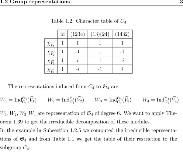
Table 1.2: Character table of C4 id (1234) (13)(24) (1432) f V1 1 1 1 1 f V2 1 -1 1 -1 f V3 1 i -1 -i f V4 1 -i -1 i
The representations induced from C4 to S4 are:
W1 = IndSC44( eV1) W2 = Ind S4 C4( eV2) W3 = Ind S4 C4( eV3) W4 = Ind S4 C4( eV4)
W1, W2, W3, W4 are representation of S4 of degree 6. We want to apply
The-orem 1.39 to get the irreducible decomposition of these modules.
In the example in Subsection 1.2.5 we computed the irreducible representa-tions of S4 and from Table 1.1 we get the table of their restriction to the
subgroup C4:
Table 1.3: Table of restrictions from S4 to C4
id (1234) (13)(24) (1432) Res( V1) 1 1 1 1 Res( V2) 1 -1 1 -1 Res( V3) 3 -1 -1 -1 Res( V4) 3 1 -1 1 Res( V5) 2 0 2 0
We can now apply Theorem 1.39:
( W1, V1)S4 = ( fV1, Res( V1))C4 = 1
( W1, V2)S4 = ( fV1, Res( V2))C4 = 0
( W1, V3)S4 = ( fV1, Res( V3))C4 = 0
( W1, V5)S4 = ( fV1, Res( V5))C4 = 1
We have calculated how many times the Vi occur in W1, so we get:
W1 ' V1 V4 V5 W1 = V1 + V4 + V5
We repeat the procedure for W2, W3, W4:
( W2, V1)S4 = ( fV2, Res( V1))C4 = 0 ( W2, V2)S4 = ( fV2, Res( V2))C4 = 1 ( W2, V3)S4 = ( fV2, Res( V3))C4 = 1 ( W2, V4)S4 = ( fV2, Res( V4))C4 = 0 ( W2, V5)S4 = ( fV2, Res( V5))C4 = 1 And then: W2 ' V2 V3 V5 W2 = V2 + V3 + V5 ( W3, V1)S4 = ( fV3, Res( V1))C4 = 0 ( W3, V2)S4 = ( fV3, Res( V2))C4 = 0 ( W3, V3)S4 = ( fV3, Res( V3))C4 = 1 ( W3, V4)S4 = ( fV3, Res( V4))C4 = 1 ( W3, V5)S4 = ( fV3, Res( V5))C4 = 0 Thus: W3 ' V3 V4 W3 = V3 + V4 ( W4, V1)S4 = ( fV4, Res( V1))C4 = 0 ( W4, V2)S4 = ( fV4, Res( V2))C4 = 0 ( W4, V3)S4 = ( fV4, Res( V3))C4 = 1 ( W4, V4)S4 = ( fV4, Res( V4))C4 = 1
( W4, V5)S4 = ( fV4, Res( V5))C4 = 0
Hence:
W4 ' V3 V4 W4 = V3 + V4
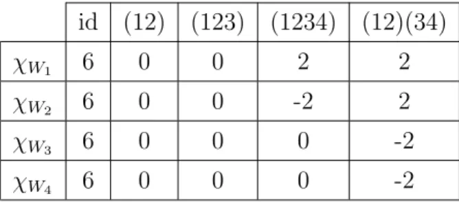
We note that W3 ' W4 and we report the character table of the induced
representations from C4 to S4.
Table 1.4: Character table of the induced representations from C4 to S4
id (12) (123) (1234) (12)(34)
W1 6 0 0 2 2
W2 6 0 0 -2 2
W3 6 0 0 0 -2
Preliminaries in Topology and
Combinatorics
2.1
Simplicial homology
In this Section we recall the fundamental definitions of simplicial homol-ogy. In the end of the Section we prove the Alexander duality.
2.1.1
Simplicial complexes
Definition 2.1. Given a set {a0, . . . , an} of points of Rp, this set is said to
be geometrically independent if for any (real) scalars ti, the equations n X i=0 ti = 0 and n X i=0 tiai = 0 imply that t0 = t1 =· · · = tn = 0.
It is clear that a one point set is always geometrically independent. Ele-mentary arguments show that in general {a0, . . . , an} is geometrically
inde-pendent if and only if the vectors
a1 a0, . . . , an a0
are linearly independent in the sense of ordinary linear algebra. Thus two distinct points in Rp form a geometrically independent set, as do three
non-collinear points, four non-coplanar points, and so on.
Definition 2.2. Given a geometrically independent set of points{a0, . . . , an},
we define the n-plane P spanned by these points as the set of all points x2 Rp
such that x = n X i=0 tiai
for some scalars ti with Pti = 1. Since the ai’s are geometrically
indepen-dent, the ti’s are uniquely determined by x. Note that each point ai belongs
to the plane P .
The plane P can also be described as the set of all points x such that x = a0+
n
X
i=1
ti(ai a0)
for some scalars t1, . . . , tn; in this form we speak of P as the plane through
a0 parallel to the vectors ai a0.
Definition 2.3. Let {a0, . . . , an} be a geometrically independent set in Rp.
We define the n-simplex spanned by a0, . . . , an as the set of all points
x2 Rp such that x = n X i=0 tiai where n X i=0 ti = 1, ti > 0.
The numbers ti’s are uniquely determined by x; they are called the
barycen-tric coordinates of the point x of with respect to a0, . . . , an.
Example 6. In low dimensions, one can easily draw a simplex. A 0-simplex is a point, of course. The 1-simplex spanned by a0 and a1 consists of all
points of the form
x = ta0+ (1 t)a1 where 06 t 6 1.
This is just the line segment joining a0 and a1. Similarly, the 2-simplex
Recall that a subset A of Rp is said to be convex if for each pair x, y of
points of A, the line segment joining them lies in A.
Let be the n-simplex spanned by{a0, . . . , an}, then the following
prop-erties hold:
1) is a compact, convex set in Rp, which equals the intersection of all
convex sets inRp containing a
0, . . . , an.
2) Given a simplex , there is one and only one geometrically independent set of points spanning .
The points a0, . . . , anthat span are called the vertices of ; the number n is
called the dimension of . Any simplex spanned by a subset of{a0, . . . , an}
is called a face of . The faces of di↵erent from itself are called the proper faces of ; their union is called the boundary of and denoted by Bd( ). The interior of is defined as Int( ) = r Bd( ).
Since Bd( ) consists of all points x of such that at least one of the barycentric coordinates ti(x) is zero, Int( ) consists of those points of for
which ti(x)> 0 for all i.
Definition 2.4. A simplicial complex K inRp is a collection of simplices in
Rp such that:
i) Every face of a simplex of K is in K.
ii) The intersection of any two simplices of K is a face of each of them. The following lemma is sometimes useful in verifying that a collection of simplices is a simplicial complex:
Lemma 2.5. A collection K of simplices is a simplicial complex if and only if the following hold:
(2) Every pair of distinct simplices of K have disjoint interiors. Proof . See [15], Lemma 2.1; pag 8.
Definition 2.6. If L is a sub-collection of K that contains all faces of its elements, then L is a simplicial complex in its own right; it is called a sub-complex of K. One sub-sub-complex of K is the collection of all simplices of K of dimension at most l; it is called the l-skeleton of K and is denoted by K(l).
The points of the collection K(0) are called the vertices of K.
Definition 2.7. Let|K| be the subset of Rp that is the union of the simplices
of K. Giving each simplex its natural topology as a subspace of Rp, we then
topologize|K| by declaring a subset A of |K| to be closed in |K| if and only if A\ is closed in , for each 2 K. It is easy to see that this defines a topology on |K|. The space |K| is called the underlying space of K, or the polytope of K.
Now we introduce the notion of a simplicial map of one complex into another.
Lemma 2.8. Let K and L be complexes, and let f : K(0) ! L(0)
be a map such that whenever the vertices v0, . . . , vn of K span a simplex of
K, the points f (v0), . . . , f (vn) are vertices of a simplex of L. Then f can
be extended to a continuous map g : |K| ! |L| as follows: for x = Pn i=0tivi g(x) = n X i=0 tif (vi)
We call g the linear simplicial map induced by the vertex map f . Proof . See [15], Lemma 2.7; pag 12.
Lemma 2.9. Suppose
is a bijective correspondence such that the vertices v0, . . . , vn of K span a
simplex of K if and only if f (v0), . . . , f (vn) span a simplex of L. Then the
induced simplicial map
g : |K| ! |L|
is a homeomorphism. Each simplex of K is mapped by g onto a simplex ⌧ of L of the same dimension as . The map g is called a simplicial homeo-morphism of K with L.
Proof . See [15], Lemma 2.8; pag 12.
2.1.2
Abstract simplicial complex
Definition 2.10. An abstract simplicial complex is a collection S of finite nonempty sets, such that if A is an element of S and B ✓ A is a nonempty subset of A then B 2 S.
The element A ofS is called a simplex of S; its dimension is one less than the number of its elements. Each nonempty subset of A is called a face of A. The dimension ofS is the largest dimension of one of its simplices, or it is infinite if there is no such largest dimension. The vertex set V of S is the union of the one-point elements of S; we shall make no distinction between the vertex v 2 V and the 0-simplex {v} 2 S. A sub-collection of S that is itself a complex is called a sub-complex of S.
Definition 2.11. Two abstract complexesS and T are said to be isomorphic if there is a bijective correspondence f mapping the vertex set of S to the vertex set ofT such that:
{a0, . . . , an} 2 S if and only if {f(a0), . . . , f (an)} 2 T
Definition 2.12. If K is a simplicial complex, let V = K(0) be the vertex
set of K. Let R be the collection of all subsets {a0, . . . , an} of V such that
the vertices a0, . . . , an span a simplex of K. The collection R is called the
The collectionR is a particular example of an abstract simplicial complex. Theorem 2.13. a) Every abstract complex S is isomorphic to the vertex
scheme of some simplicial complex K.
b) Two simplicial complexes are simplicial homeomorphic if and only if their vertex schemes are isomorphic as abstract simplicial complexes. Proof . See [15], Theorem 3.1; pag 15.
Definition 2.14. If the abstract simplicial complex S is isomorphic to the vertex scheme of the simplicial complex K, we call K a geometric realization of S. It is uniquely determined up to simplicial homeomorphism.
Example 7. Let v1, v2 be two independent vectors inR2 and let
={v1, v2, v1+ v2, 2v1+ v2}.
We now consider the collection of independent subsets of :
S =n{v1, v2}, {v1, v1+ v2}, {v1, 2v1+ v2}, {v2, v1+ v2}, {v2, 2v1+ v2},
{v1+ v2, 2v1+ v2}, {v1}, {v2}, {v1+ v2}, {2v1+ v2}
o The collection S is an abstract simplicial complex.
2.1.3
Homology groups
Definition 2.15. Let be a simplex (either geometrical or abstract). We define two orderings of its vertex set to be equivalent if they di↵er from one another by an even permutation. If dim( ) > 0, the orderings of the vertices of then fall into two equivalence classes. Each of these classes is called an orientation of . (If is a 0-simplex, then there is only one class and hence only one orientation of .)
An oriented simplex is a simplex together with an orientation of .
If the points v0, . . . , vp are geometrically independent, we shall use the
sym-bol:
to denote the simplex they span, and we shall use the symbol [v0. . . vp]
to denote the oriented simplex consisting of the simplex v0. . . vp and the
equivalence class of the particular ordering (v0. . . vp).
Definition 2.16. Let K be a simplicial complex. A p-chain of K is a function cp from the oriented p-simplices of K to the integers, such that:
i) cp( ) = cp( 0) if and 0 are opposite orientations of the same simplex.
ii) cp( ) = 0 for all but finitely many oriented p-simplices .
We add p-chains by adding their values; the resulting group is denoted by Cp(K) and is called the group of (oriented) p-chains of K. If p < 0 or
p > dim(K) we let Cp(K) denote the trivial group.
If is an oriented simplex, the elementary chain c corresponding to is a function defined as follows:
c( ) = 1
c( 0) = 1 if 0 is the opposite orientation of , c(⌧ ) = 0 for all other oriented simplices ⌧ .
By abuse of notation, we often use the symbol to denote not only a simplex, or an oriented simplex, but also to denote the elementary p-chain c corresponding to the oriented simplex . With this convention, if and
0 are opposite orientation of the same simplex, then we can write 0 = ,
because this equation holds when and 0 are interpreted as elementary chains.
Lemma 2.17. Cp(K) is free abelian: a basis for Cp(K) can be obtained by
orienting each p-simplex and using the corresponding elementary chain as a basis.
Proof . See [15], Lemma 5.1; pag 28.
The group C0(K) di↵ers from the others, since it has a natural basis (since
a 0-simplex has only one orientation). The group Cp(K) has no natural basis
if p > 0; one must orient the p-simplices of K in some arbitrary fashion in order to obtain a basis.
Definition 2.18. We now define a homomorphism @p : Cp(K) ! Cp 1(K)
called the boundary operator. If = [v0, . . . , vp] is an oriented simplex with
p > 0, we define @p( ) = @p([v0, . . . , vp]) = p X i=0 ( 1)p[v0, . . . , ˆvi, . . . , vp] (2.1)
where the symbol ˆvi means that the vertex vi is to be deleted from the array.
Since Cp(K) is the trivial group for p < 0, the operator @p is the trivial
homomorphism for p6 0
We must check that @p is well-defined and that p( ) = @p( ). For
this purpose, it suffices to show that the right side of Equation (2.1) changes sign if we exchange two adjacent vertices in the array [v0, . . . , vp]. So let us
compare the expressions for
p([v0, . . . , vj, vj+1, . . . , vp]) and p([v0, . . . , vj+1, vj, . . . , vp])
For i 6= j, j + 1, the ith terms in these two expressions di↵er precisely by a sign; the terms are identical except that vj and vj+1 have been interchanged.
What about the ith terms for i = j and i = j + 1? In the first expression, one has:
( 1)j[. . . , vj 1, ˆvj, vj+1, vj+2, . . . ] + ( 1)j+1[. . . , vj 1, vj, ˆvj+1, vj+2, . . . ]
In the second expression, one has:
( 1)j[. . . , vj 1, ˆvj+1, vj, vj+2, . . . ] + ( 1)j+1[. . . , vj 1, vj+1, ˆvj, vj+2, . . . ].
Example 8. For a 1-simplex, we have
@1([v0, v1]) = v1 v0
For a 2-simplex one has:
@2([v0, v1, v2]) = [v1, v2] [v0, v2] + [v0, v1]
Lemma 2.19. @p 1 @p = 0
Proof . See [15], Lemma 5.3; pag 30. Definition 2.20. The kernel of
@p : Cp(K) ! Cp 1(K)
is called the group of p-cycles and denoted by Zp(K). The image of
@p+1: Cp+1(K) ! Cp(K)
is called the group of p-boundaries and is denoted by Bp(K). By Lemma
2.19, each boundary of a p + 1 chain is automatically a p-cycle. That is, Bp(K)⇢ Zp(K). We define
Hp(K) = Zp(K)/Bp(K)
and call it the pth homology group of K.
Theorem 2.21. Let K be a complex. Then the group H0(K) is free abelian.
If{v↵} is a collection consisting of one vertex from each connected component
of |K|, then the homology classes of the chains v↵ form a basis for H0(K).
Proof . See [15], Theorem 7.1; pag 41.
It is convenient to consider another version of the 0-dimensional homology. Definition 2.22. Let
be the surjective homomorphism defined by ✏(v) = 1 for each vertex v of K. Then if c is a 0-chain, ✏(c) equals the sum of the values of c on the vertices of K. The map ✏ is called the augmentation map for C0(K). We have just
noted that ✏(@(d)) = 0 if d is a 1-chain. We define the reduced homology group of K in dimension 0, denoted by eH0(K), by the equation:
e
H0(K) = ker(✏)/Im(@1)
If p > 0, we let eHp(K) denote the usual group Hp(K).
The relation between reduced and ordinary homology is as follows: Theorem 2.23. The group eH0(K) is free abelian, and
e
H0(K) Z ' H0(K)
Thus eH0(K) vanishes if |K| is connected. If |K| is not connected, let {v↵}
consist of one vertex from each component|K|, let ↵0 be a fixed index. Then
the homology classes of the chains v↵ v↵0, for ↵ 6= ↵0, form a basis for
e H0(K).
Proof . See [15], Theorem 7.2; pag 43.
2.1.4
Homology groups with arbitrary coefficients
Definition 2.24. Let R be an abelian group. Let K be a simplicial complex. A p-chain of K with coefficients in R is a function cp from the oriented
p-simplices of K to R, such that:
i) cp( ) = cp( 0) if and 0 are opposite orientations of the same simplex;
ii) cp( ) = 0 for all but finitely many oriented p-simplices .
We add p-chains by adding their values; the resulting group is denoted by Cp(K; R) and is called the group of (oriented) p-chains of K with coefficients
If is an oriented simplex and if g 2 R, we denote by g the elementary chain defined as follows:
- g ( ) = g
- g ( 0) = g if 0 is the opposite orientation of
- g (⌧ ) = 0 for all other oriented simplices ⌧ .
If one orients all the p-simplices of K, then each chain cp can be written
uniquely as a finite sum
cp =
X
i
gi i
of elementary chains. Thus Cp(K, R) is the direct sum of subgroups
isomor-phic to R, one for each p-simplex of K. The boundary operator
@p : Cp(K, R) ! Cp 1(K, R)
is defined easily by the formula:
@p(g ) = g@p( )
where @p( ) is the ordinary boundary, defined earlier. As before, = 0
and we define Zp(K, R) to be the kernel of the homomorphism:
@p : Cp(K, R) ! Cp 1(K, R).
Furthermore we define Bp(K, R) to be the image of the following
homomor-phism:
@p 1 : Cp 1(K, R) ! Cp(K, R)
and
Hp(K, R) = Zp(K, R)/Bp(K, R)
These groups are called the group of the cycles, the group of the boundaries, and the homology group of K with coefficients in R respectively.
Of course, one can also study reduced homology with coefficients in R. The details are clear.
2.1.5
Cohomology groups
Associated with any pair of abelian groups A, G is a third abelian group, the group Hom(A, G) of all homomorphism of A into G. In this subsection we study some of its properties.
Definition 2.25. If A and G are abelian groups, then the set Hom(A, G) of all homomorphism of A into G becomes an abelian group if we add two homomorphisms by adding their values in G.
Definition 2.26. A homomorphism f : A ! B gives rise to a dual homomorphism
e
f : Hom(B, G) ! Hom(A, G)
going in the reverse direction. The map ef assigns to the homomorphism : B ! G , the composite
e
f ( ) : A ! B ! G.f That is, ef ( ) = f .
Definition 2.27. In the context of group theory, a sequence G0 f1 ! G1 f2 ! G2 · · · fn ! Gn
of groups and group homomorphism is called exact if the image of each homomorphism is equal to the kernel of the next:
Im(fk) = Ker(fk+1)
Note that the sequence of groups and homomorphisms may be either finite or infinite.
Example 9. If the following sequence
0 ! A! Bf ! C ! 0g
is exact then f is an injective homomorphism and g is a surjective homomor-phism. Furthermore:
Theorem 2.28. Let G be an abelian group. Let f be a homomorphism, let e
f be the dual homomorphism. Then: a) If f is an isomorphism, so is ef .
b) If f is the zero homomorphism, so is ef .
c) If f is surjective, then ef is injective. That is the exactness of B ! C ! 0f
implies the exactness of
Hom(B, G) Hom(C, G) 0fe Proof . See [15], Theorem 41.1; pag 247.
Now we can give the definition of cohomology groups.
Definition 2.29. Let K be a simplicial complex; let R be an abelian group. The group of p-dimensional cochains of K, with coefficients in R, is the group
Cp(K, R) = Hom(C
p(K), R)
The coboundary operator p+1 is defined to be the dual of the boundary
operator @p+1 : Cp+1(K) ! Cp(K) . Thus
p+1 : Cp(K, R) ! Cp+1(K, R)
so that p+1 raises dimension by one. We define Zp(K; R) to the kernel of
this homomorphism, Bp+1(K, R) to be its image, and (noting that 2 = 0
because @2 = 0),
Hp(K; R) = Zp(K; R)/Bp(K; R)
These groups are called the group of cocycles, the group of coboundaries, and the cohomology group, respectively, of K with coefficients in R.
If cp is a p-dimensional cochain, and c
p is a p-dimensional chain, we
com-monly use the notation
hcp, cpi = cp(cp).
Proposition 2.30. Using the same notation as above, the definition of the coboundary operator becomes:
h p+1(cp), dp+1i = hcp, @p+1(dp+1)i
Proof . We have:
@p+1: Cp+1(K) ! Cp(K)
dp+1 7 ! @p+1(dp+1)
and p+1 is its dual map:
p+1: Cp(K) ! Cp+1(K) cp 7 ! p+1(cp) By definition we have: p+1(cp) = cp @p+1 and so: p+1(cp)(dp+1) = (cp @p+1)(dp+1) = cp(@p+1(dp+1))
Definition 2.31. Given a complex K, we dualize the standard augmentation map C1(K) @1 ! C0(K) ✏ ! Z and obtain a homomorphism e✏:
C1(K) 1
C0(K) Re✏
called a coaugmentation. It is injective, and 1 e✏ = 0. We define the reduced
cohomology of K by setting: e
Hq(K; R) = Hq(K; R) if q > 0 and
e
Theorem 2.32. If |K| is connected, then eH0(K; R) = 0. More generally,
for any complex K, we have:
H0(K; R) ' eH0(K; R) R Proof . See [15], Theorem 42.2; pag 256.
Proposition 2.33. Let K be a simplicial complex. Let F be a field. Then e
Hp(K,F) and eHp(K,F)
have the structure of vector spaces over F. They are dual of each other as vector spaces. Besides, both and @ are vector space homomorphisms (linear transformations).
Proof . See [15]; pag 324.
2.1.6
Homomorphism induced by a simplicial map
If f is a simplicial map of|K| into |L|, then f maps each p-simplex i of
K onto a simplex ⌧i of L of the same or lower dimension. We shall define
a homomorphism of p-chains that carries a formal sum Pimi i of oriented
p-simplices of K onto the formal sum Pimi⌧i of their images. (We delete
form the latter sum those simplices ⌧i whose dimension is less than p.) This
map in turn induces a homomorphism of homology groups. As a general notation, we shall use the phrase
00 f : K ! L is a simplicial map00
to mean that f is a continuous map of |K| into |L| that maps each simplex of K linearly onto a simplex of L. Thus f maps each vertex of K to a vertex of L, and it equals the simplicial map induced by this vertex map.
Definition 2.34. Let f : K ! L be a simplicial map. If v0. . . vp is
a simplex of K, then the points f (v0), f (v1), . . . , f (vp) span a simplex of L.
We define a homomorphism
by defining it on oriented simplices as follows: f#([v0, . . . , vp]) = 8 < : [f (v0), . . . , f (vp)], if f (v0), . . . , f (vp) are distinct 0, otherwise
This map is clearly well-defined; exchanging two vertices in the expression [v0, . . . , vp] changes the sign of the right side of the equation. The family
of homomorphisms {f#}, one in each dimension, is called the chain map
induced by the simplicial map f .
Lemma 2.35. The homomorphism f# commutes with @; therefore f#
in-duces a homomorphism
f⇤ : Hp(K) ! Hp(L)
Proof . See [15], Lemma 12.1; pag 62.
Lemma 2.36. The chain map f# preserves the augmentation map ✏;
there-fore it induces a homomorphism
f⇤ : Hep(K) ! eHp(L)
of reduced homology groups.
Proof . See [15], Lemma 12.3; pag 63.
2.1.7
Alexander Duality
Let K be an abstract simplicial complex with ground set V . For 2 K, let
= V r
Definition 2.37. The Alexander dual of K is the simplicial complex on the same ground set defined by
K⇤ ={ ✓ V | 2 K}/ It is easy to see that K⇤⇤ = K.
Let K be a simplicial complex with ground set V ={1, 2, . . . , n}. For j 2 2 K, we define the sign
sgn(j, ) = ( 1)i 1
where j is the ith smallest element of the set . The following simple property of the sign function will be needed.
Lemma 2.38. Let k2 ✓ {1, 2, . . . , n} and p( ) =Qi2 ( 1)i 1. Then
sgn(k, ) p( r k) = sgn(k, [ k) p( ) Proof . sgn(k, )sgn(k, [ k) =Y i2 i<k ( 1) Y i2 i<k ( 1) = ( 1)k 1 and p( )p( r k) =Y i2 ( 1)i 1 Y i2 rk ( 1)i 1= ( 1)k 1 We have also: sgn(k, )sgn(k, [ k) p( )p( r k) = ( 1)k 1 ( 1)k 1 = 1 sgn(k, )sgn(k, [ k) p( )p( r k) = ( 1)2k 2= 1 We obtain then: p2( )p2( r k) = 1 =) p2( ) = 1 and p2( r k) = 1 sgn2(k, )sgn2(k, [ k) = 1 =) sgn2(k, ) = 1 and sgn2(k, [ k) = 1 sgn(k, ) p( r k) = sgn(k, ) p( r k) sgn2(k, [ k) p2( ) = = ( 1)k 1 ( 1)k 1 sgn(k, [ k) p( ) = sgn(k, [ k) p( )
We now review the definitions and notation used for (co)homology. Through-out this subsection we suppose that R is a commutative ring containing a unit element. In particular R could also be a field F.
Definition 2.39. Let Ci = Ci(K) be a free R-module with the free basis
{e | 2 K, dim( ) = i}. The reduced chain complex of K over R is the complex
e C⇤(K) = eC⇤(K, R) =· · · Ci+1 @i+1 ! Ci @i ! Ci 1 ! · · · , i2 Z
whose mappings @i are defined as
@i(e ) =
X
j2
sgn(j, )e rj.
The complex eC⇤(K) is formally infinite; however Ci = 0 for i < 1 or
i > dim(K). The nth reduced homology group of K over R is e
Hn(K) = eHn(K; R) = ker(@n)/Im(@n+1).
Definition 2.40. Let Ci = Ci(K) be a free R-module with free basis
{e⇤ | 2 K, dim( ) = i}. The reduced cochain complex of K over R is the complex
e
C⇤(K) = eC⇤(K, R) =· · · Ci 1 i
! Ci i+1! Ci+1 ! · · · , i2 Z where i = @i⇤ are maps dual to @i, explicitly stated:
i(e⇤) =
X
j /2 [j2K
sgn(j, [ j)e⇤[j The nth reduced cohomology group over R is
e