1
ALMA MATER STUDIORUM
UNIVERSITÀ DI BOLOGNA
FACOLTÀ DI SCIENZE MATEMATICHE FISICHE E NATURALI
Corso di laurea magistrale in BIOLOGIA MARINA
Modelling growth dynamics and toxin production in
Ostreopsis cf. ovata
Relatore: Presentata da:
Prof.ssa Rossella Pistocchi Adriano Pinna
Correlatori:
Dott.ssa Laura Pezzolesi
Dott. Luca Polimene
(III sessione)
3
INDEX
1. INTRODUCTION ……… 5 1.1 The toxic dinoflagellate Ostreopsis ovata ……….. 5
1.1.1 Geographical distribution, morphological description, and ecology of O. ovata 5
1.1.2 Toxins produced by O. ovata 8
1.1.3 O. cf. ovata blooms in the Mediterranean Sea and dangers for public health 10
1.1.4 Bloom and toxin production dynamics of O. cf. ovata 13
1.2 The ‘European Regional Seas Ecosystem Model (ERSEM)’……….. 15
1.2.1 An overview of ERSEM 15
1.2.2 Development of ERSEM and a few technical features 17
2. AIMS OF THIS STUDY………... 19 3. MATERIALS AND METHODS ………. 20 3.1 The experiment Beta ……….. 20
3.1.1 Experimental plan 20
3.1.2 Cell counts and biovolumes 22
3.1.3 Chlorophyll-a 24
3.1.4 Analysis of dissolved inorganic nutrients and organic phosphorus 25
3.1.5 Polysaccharides 27
3.1.6 Elemental analysis (CHN) 27
3.1.7 Toxins 28
3.1.8 Cell counts and biovolumes of bacteria 28
3.2 Preparations required for the modelling ……….. 29
3.2.1 Experiments "Alpha" & "Beta" and converting Units of Measure 29
3.2.2 Data processing 30
3.3 Modelling ………. 32
3.3.1 General setting of ERSEM and initial conditions 32
3.3.2 Modelling toxin production and excretion 34
3.3.3 Chlorophyll, rest respiration and mortality 36
3.3.4 Parameter setting 39
3.3.5 Used software and statistics 41
4. RESULTS AND DISCUSSION ………... 42 4.1 The experiment Beta ……….. 42
4.1.1 Growth curves and cell volumes 42
4.1.2 Chlorophyll-a 44
4.1.3 Inorganic nutrient 45
4.1.4 Polysaccharides 46
4.1.5 Organic carbon, nitrogen and phosphorus in O. cf. ovata cells 47
4.1.6 Toxins 50
4.1.7 Growth curve and cell volume of bacteria 52
4
4.2.1 O. cf. ovata tolerance to nutrient deficiency-stress 53
4.2.2 O. cf. Ovata toxicity 55
4.2.3 Results from the processing to organic carbon values 56
4.3 Simulating the experiment Alpha ………. 57
4.3.1 A first run of ERSEM 57
4.3.2 Results of the modelling work 59
4.3.3 Sensitivity tests 62
4.4 Simulating the experiment Beta ……… 64
4.4.1 The simulation and its gaps 64
4.4.2 Possible explanations of gaps and further changes to the model 66
5. CONCLUSIONS ………... 70 ACKNOWLEDGEMENTS ………. 72 REFERENCES ………. 73
5
1. INTRODUCTION
1.1 The toxic dinoflagellate Ostreopsis ovata
1.1.1 Geographical distribution, morphological description and ecology of O. ovata
The genus Ostreopsis Schmidt, together with the genus Coolia Meunier, composes the family of Ostreopsidaceae, order Gonyaulacales, class Dinophyceae, phylum Dinophyta.
Ostreopsis genus is actually represented by 9 species of marine dinoflagellates, some of which are toxic (condition here indicated with t ): O. siamensis t Schmidt (1901), O. ovata t Fukuyo (1981), O. lenticularis t Fukuyo (1981), O. heptagona t Norris, Bomber and Balech (1985), O. mascarenensis t Quod (1994), O. labens t Faust and Morton (1995), O. marinus Faust (1999), O. belizeanus Faust (1999), and O. caribbeanus Faust (1999) (Penna et al., 2005).
The aforementioned toxicity of some species belonging to this genus, their ability to develop large blooms, and an apparent increase in their distribution range (at least for some species), make them an interesting subject of study (Rhodes, 2011).
The species of the genus Ostreopsis, as many other dinoflagellates, are mostly distinguished for morphological traits, like form and dimension of the cells, plates type and number, and incisions on these lasts. However, because of a quite high intra-specific morphological variability, and a relative similarity between some species, sometimes molecular analysis could be required to distinguish between them (Pin et al., 2001; Battocchi et al., 2010; Penna et al., 2012); moreover molecular studies could also give useful information about phylogeny and biogeography of the species.
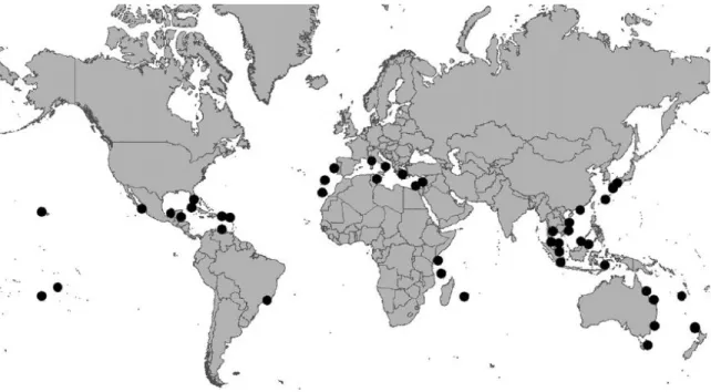
Ostreopsis spp. dinoflagellates have a nearly worldwide distribution in tropical areas of the oceans, and are also diffused in some temperate waters (Japan, Southern Australia, New Zealand, Mediterranean Sea) (Fig. 1) where recently they have caused several blooms (Faust et al., 1996; Shears & Ross, 2009; Rhodes, 2011).
To date, in the Mediterranean Sea have been recovered only two species belonging to the Ostreopsis genus: O. cf. siamensis Schmidt in the 70s (Taylor, 1979) and O. cf. ovata Fukuyo in the 90s (Tognetto et al., 1995).
6
Figure 1. Distribution across the world of the dinoflagellates belonging to the Ostreopsis genus (from Rhodes, 2011).
An Adriatic Ostreopsis cf. ovata strain is the subject of this study.
In recent times this dinoflagellate has been studied quite extensively in many aspects by scientists [Vila et al., 2001; Turki, 2005; Ciminiello et al., 2006; Riobó et al., 2006; Guerrini et al., 2010; special issue on Ostreopsis in Toxicon, 57 (2001); and many others] because of its increasing diffusion along densely populated temperate coasts, coupled to its ability in producing toxins (see the following section 1.1.2 and 1.1.3).
O. cf. ovata is present in many tropical areas, and with regard to the Mediterranean Sea it has been found in high concentrations during the two last decades along the coasts of Spain (Penna et al., 2005; Bravo et al., 2012), France (Sechet et al., 2012; Cohu et al., 2013), Italy (Tognetto et al., 1995; Mangialajo et al., 2008; Totti et al., 2010), Croatia (Monti et al., 2007; Bravo et al., 2012), Greece (Aligizaki & Nikolaidis, 2006) and Tunisia (Turki, 2005; Sechet et al., 2012). It is still not clear if this alga has reached and colonized the Mediterranean Sea recently, transported from tropical seas via ballast-waters of ships, or if it was already present but at very low cell density, since bloom of this species were not recorded before the 90s. From some molecular studies, based on the LSU(D1/D2) - ITS - 5.8S rDNAs of some Ostreopsis spp. and Coolia monotis (considered as an outgroup reference) performed on several samples from different areas of the Mediterranean and eastern Atlantic coasts, resulted that O. cf. ovata has a single panmictic population for these areas, quite distinct from populations of the Indo-Pacific (Penna et al., 2010; Penna et al., 2012). This result leads to suppose that a well-structured Mediterranean/Eastern-Atlantic population was
7 already present for long time, therefore being not a recent colonization from tropical sea. Qualitative and quantitative molecular assays, as seen, can be extremely sensitive and could improve geographical distribution studies on Ostreopsis spp. in the future (Penna et al., 2007).
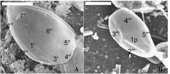
About morphology, O. ovata is a thecate dinoflagellate of medium size, with color ranging from ocher to dark brown: as the name suggests, this alga is oval to tear shaped, pointed to the ventral side, with an ephitheca which is equal in size to the hypotheca, both composed of thin and delicate thecal plates (Fig. 2). Although it was observed an high intra-specific morphometric variability, especially in clonal cultures (less in field samples), it has been possible to determine some distinguishing features of this species. In Penna et al. (2005) and Aligizaki & Nikolaidis (2006) cells of different O. cf. ovata strains were compared to cells of several strains of the most similar species, O. cf. siamensis: O. cf. ovata resulted to have a DV diameter ranging between 26 and 65 μm, a width from 13 to 57 μm, and an AP diameter from 14 to 36 μm, with DV/AP ratios lower than 2. Considering its mean size, this dinoflagellate is the smallest among the species of the genus Ostreopsis. Observing the cells with Scanning Electron Microscopy (SEM) the thecal surface results smooth and also covered with spaced pores. O. cf. ovata complete plate pattern, which is crucial in distinguishing the species from other dinoflagellate, is « Po, 3’ , 7’’, 6C, 6S, 5’’’, 2’’’’, 1p » as reported in Faust & Gulledge (2002) (Fig. 2).
Figure 2. O. cf. ovata observed with the SEM (Aligizaki & Nikolaidis, 2006). Epithecal (A) and hipothecal (B) view and relative plates. White scale bar of 20 μm.
Regarding its ecology, O. ovata is a mixotrophic benthic dinoflagellate, auxotrophic for some vitamins, able to phagocytize its preys (bacteria, ciliates, other microalgae) using an expandable ventral pore (Faust, 1998). As suggested by Nikolaidis & Aligizaki (2006), O. cf. ovata could be
8
able to enter in a resting stage, forming a sort of cysts, as demonstrated by the presence of some red hyaline bodies in many large field cells (that are candidates to turn into cysts, in contrast to small cells that are typically found during blooms, or prosperous periods), and by the fact that some cysts have been already observed in the related species O. cf. siamensis (Pearce et al., 2001) and C. monotis (Faust, 1992). In senescent cultures of O. cf. ovata some small spherical cells surrounded by a gelatinous envelope, that could be identified as cysts (Simoni et al., 2004), have been observed, but further and more specific studies would be needed to shed light on this aspect in O. cf. ovata life cycle.
This alga prefers to reside in shallow and calm waters, as it apparently requires high levels of light and warm waters (Totti et al., 2010), living as epiphyte of other sessile organisms or free on many kinds of hard substrata (Pistocchi et al., 2011).
In tropical areas, this dinoflagellate is particularly present in coral reef lagoon environments (Faust et al., 1996) as component of the epiphytic/benthic microflora on corals/sand, often in association with other Ostreopsis spp., and Gambierdiscus, Prorocentrum, Amphidinium species, with which has been implicated in causing the syndrome of ciguatera in humans (Morton et al., 1992).
In the Mediterranean Sea (but also in other temperate areas, like southern Australia, New Zealand, and Japan), O. cf. ovata is frequent as epiphyte on seagrasses and red-brown macrophytes that live in sheltered coves, especially along rocky shores. O. cf. ovata blooms typically occur during warm periods, with high temperature and salinity, and low hydrodynamism (Pistocchi et al., 2011). During the development of the bloom, by taking advantage of calm waters, O. cf. ovata covers all benthic substrates forming a mucilaginous film, which is composed by a fibrillar part made of cells’ trichocysts and a mucilage part (Honsell et al., 2013). Cells are easily re-suspended in the water column if the hydrodynamism increases (Mangialajo et al., 2008; Totti et al., 2010; Mangialajo et al., 2011) in fact the hydrodynamism seems to have an important role in the development and decline of blooms (Aligizaki & Nikolaidis, 2006; Mangialajo et al., 2008).
1.1.2 Toxins produced by O. ovata
Palytoxin (PLTX) is a potent non-protein marine toxin, initially isolated in 1971 from some
Palythoa spp., soft corals of the Pacific Ocean (Moore & Scheuer, 1971; Uemura et al., 1981). Since 70s, PLTX and a number of palytoxin analogues have been extracted also from many other marine organisms, including O. ovata and other dinoflagellates of the same genus (Ciminiello et al., 2011a,b).
9 PLTX is a large and very complex molecule with chemical composition C129H233N3O54, formed by
a long polyhydroxylated and partially unsaturated aliphatic backbone, containing 64 chiral centers (Ramos & Vasconcelos, 2010). High resolution liquid chromatography - mass spectrometry (HR LC-MS) studies disclosed the presence, both in field (from Mediterranean areas) and cultured O. cf. ovata cells, of putative PLTX and six new palytoxin analogues, named ovatoxins (OVTXs; Fig. 3). The ovatoxins discovered until now (Ciminiello et al., 2006, 2008, 2010, 2011a,b, 2012a,b) are all similar to the palytoxin in structure and composition :
OVTX-a, with chemical composition C129H223N3O52. It appears to be the most produced
toxin by O. cf. ovata: OVTX-a alone accounts for more than 50% of the total toxin in cultured cells (Guerrini et al., 2010; Pezzolesi et al., 2012; Ciminiello et al., 2012a; this work)
OVTX-b, with chem. comp. C131H227N3O53
OVTX-c, with chem. comp. C131H227N3O54
OVTX-d/-e, both with chem. comp. C129H223N3O53 but different structure
OVTX-f, with chem. comp. C131H227N3O52. This last was discovered in 2012 in only one
Adriatic O. cf. ovata strain, accounting alone for 50% of the total toxin content (Ciminiello et al., 2012b).
Figure 3. Molecular structure of palytoxin (PLTX) and some palytoxin-like compounds, including ovatoxin-a (OVA-a) (Del Favero et al., 2012)
10
Palytoxin and its analogues may enter the food chain and accumulate mainly in filter-feeders molluscs, fishes and crustaceans, causing severe human intoxication and death due to the ingestion of contaminated products (Alcala et al., 1988; Onuma et al., 1999). Furthermore, toxic effects in individuals exposed via inhalation or skin contact to marine aerosol in coincidence with Ostreopsis spp. blooms, have been reported (see the following section 1.1.3).
At the cellular level, the Na+/K+–ATPase is the primary molecular target of PLTX: this compound binds the Na+/K+–ATPase and convert it into a non-selective ion channel (Habermann, 1989; Rossini & Bigiani, 2011), causing the membrane depolarization and consequent Ca2+ influx that may lead to multiple events regulated by Ca2+-dependent pathways (Monroe & Tashjian, 1995). Depending on the cell type and toxin dose, also filamentous actin (F-actin) disassembly, cell rounding and swelling, cell death, and hemolytic activity have been described (Louzao et al., 2007; Prandi et al., 2011; Vidyarathna & Granéli, 2013). Furthermore, PLTX has been demonstrated to act as a skin tumor promoter, being able to modulate key signal transduction pathways involved in carcinogenesis (Fujiki et al., 1986; Wattenberg, 2007). Finally, administration of semi-purified toxic extracts from O. cf. ovata cultured cells (containing both PLTX and ovatoxins at known concentrations) in primary human macrophages induces a significant accumulation of gene transcripts the products of which are involved in inflammatory immune response (Crinelli et al., 2012), and demonstrates that palytoxin and, most likely, its congener O. cf. ovata toxins, have the potential to exert a pro-inflammatory activity.
1.1.3 O. cf. ovata blooms in the Mediterranean Sea and dangers for public health
HABs, or Harmful Algal Blooms, are blooms that cause harm, either due to the production of toxins by the blooming algae and/or to the manner in which the cells’ physical structure, or accumulated biomass, affects co-occurring organisms and alters food web dynamics, so threaten the ecology of an area. Impacts of these phenomena could include mass mortalities of wild and farmed fish, shellfish and other invertebrates; human illness and death due to the ingestion of toxic seafood or to toxin exposure through inhalation or water contact; illness and death of marine mammals, seabirds, and other animals; alteration of marine habitats and trophic structure (Anderson et al., 2002).
From the 90s to today O. cf. ovata has been responsible for several HABs in the Mediterranean Sea: its toxins caused several issues to the other organisms who used to live in the blooming coastal areas and public health problems.
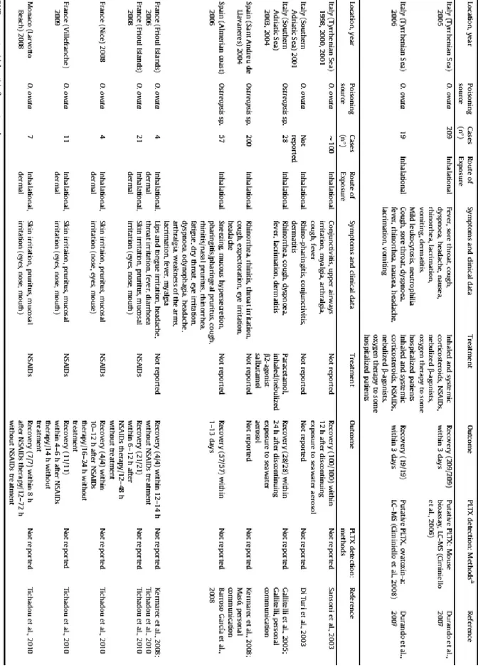
11 Human illness and death due to consumption of seafood contaminated with palytoxin and/or its analogues have been reported in tropical and subtropical zones, but not in the Mediterranean basin: here all the reported poisonings were due exclusively to exposure to seawater and/or aerosol containing palytoxins and analogues during Ostreopsis spp. blooms (Tubaro et al., 2011). In particular, since the end of the last decade, massive blooms of Ostreopsis spp. occurred along the Italian, French and Spanish coastlines during the warm season, sometimes resulting in respiratory and febrile syndrome outbreaks in humans exposed to sea-spray aerosol, which contains fragments of algal cells and/or PLTXs, and to seawater during recreational activities (see Table 1 in the next page).
The most serious incident occurred in the coasts of Genoa (Italy) between 17 and 26 July 2005, when a total of 209 subjects matched the above-described case definition. The clinical picture was mainly characterized by fever, irritative symptoms of the upper and lower respiratory tracts, conjunctives, headache, nausea and vomiting, variously associated. Mean onset of symptoms was about 4h after the beginning of exposure. In this episode forty-three subjects needed hospitalization (Durando et al., 2007).
From an ecological point of view, O. cf. ovata blooms in the Mediterranean have caused severe mass mortalities of benthic organisms (Di Turi et al., 2003; Sansoni et al., 2003; Simoni et al., 2003; Congestri et al., 2006; Shears and Ross, 2009). For example in Italy massive mortalities of marine invertebrates and macroalgae (Vale and Ares, 2007), and visible impacts on sessile (cirripeds, mussels, limpets) and mobile (echinoderms, cephalopods, little fishes) epibenthic organisms were observed after summer blooms of this dinoflagellate (Ciminiello et al., 2006; Totti et al., 2010). Despite this observed biological impact, little is known about the real consequences that these toxins may have on coastal communities: it should be considered that a damage to a single ecologically important species may rebound through the whole ecosystem, thus further investigations about toxic effects of PLTX and its analogues on different biological models (or single key-species) would be needed, as already done in some successful studies (Morton et al., 1982; Vale and Ares, 2007; Shears and Ross, 2009; Rhodes et al., 2000, 2002; Malagoli et al., 2008; Simoni et al., 2004; Faimali et al., 2011).
12
13
1.1.4 Bloom and toxin production dynamics of O. cf. ovata
There are many physical, chemical and biological factors that may affect an algal bloom.
Temperature is one of these factors, as it is important in defining the biogeographic boundaries
within which a species can live (Dale et al. 2006). Therefore, different strains of the same species can be expected to have different optimal temperatures for growth: this may be attributed to genetic adaptations to local environmental conditions (Vidyarathna & Granéli, 2012). This adaptation may explain the observed differences in growth and toxicity of various strains of O. cf. ovata at different temperatures. In fact, a Japanese O. cf. ovata strain (Vidyarathna & Granéli, 2012) reported the greatest cellular growth and the highest toxicity at temperature of 24-25° C, while two other experiments on a Thyrrhenian strain (Granéli et al., 2011) and an Adriatic strain (Pezzolesi et al., 2012) revealed maximal toxicity at 20° C and 25° C, respectively, and maximal growth at 26-30° C and 20° C, respectively.
Salinity was also considered one of the most important key-factors in determining the blooming
dynamics for this species but, as seen for temperature, field data are conflicting and depend on the considered area (i.e. strains). In addition, salinity alone seems not to explain O. cf. ovata proliferations: along Hawaiian coasts it was observed a negative correlation between salinity and O. cf. ovata presence (Parsons & Preskitt, 2007), while in the Mediterranean Sea this correlation results positive, since blooms occurred during warm periods which are characterized by higher salinity (37-39 PSU) than the annual averages (35 PSU) (Vila et al., 2001; Ungaro et al., 2005; Monti et al., 2007; Mangialajo et al. 2008; Pistocchi et al., 2010, 2011). An experiment conducted on an Adriatic O. cf. ovata strain by Pezzolesi et al. (2012), confirmed the natural trend observed in the Mediterranean areas: the greatest growth (although not so different from the others) was observed at the highest salinities of 36 and 40 PSU, while the highest toxicity at a lower salinity of 32 PSU.
Another factor, maybe the most important, in regulating algal bloom dynamics is the concentration of inorganic nutrients, primarily Nitrogen and Phosphorus. Also for this aspect field data are not clear, indeed O. cf. ovata blooms have occurred both in oligotrophic than in eutrophic waters (Vila et al., 2001; Shears & Ross, 2009; Accoroni et al., 2011). Some experiments have been conducted in order to investigate the role of nutrients in O. cf. ovata growth and toxicity, but the results were apparently conflicting. Using an Adriatic strain, Vanucci et al. (2012b) observed both the highest cellular growth and toxicity in balanced N:P conditions (molar N:P=16 in the culture medium), followed by P-deficiency (N:P=92) and N-deficiency (N:P=5) conditions. Vidyarathna & Granéli
14
(2013) instead, evidenced a significantly higher cells’ toxicity of a Tyrrhenian strain in N-limited conditions (N:P=1,6). The differences between these results could be due to the both different experimental conditions and methods adopted in the two experiments and to the different physiologies of the two O. cf. ovata strains.
Due to the complex regulation of primary metabolic processes, it is not easy to predict the conditions which promote or depress the synthesis of toxins. In general, growth dynamics and toxicity of dinoflagellates reflect the physiological status of the organism; however little is presently known about the role that these compounds play in the biology of the algal cell.
An important factor in causing the end of an algal bloom, at least in a planktonic context, is the
grazing pressure: for O. cf. ovata, which is a toxic benthic microalga, the role of grazing might
decrease, since during its blooms mass mortalities of its potential predators, like sea-urchins and other benthic invertebrates, have been observed, due to the toxin production (Totti et al., 2010; and references therein).
Nevertheless it could be also possible that O. cf. ovata is influenced by substances produced by other organisms, in a positive or negative manner (allelopathy). For example, it is known that some of the species that are often associated to O. ovata (Amphidinium sp., Coolia monotis, Gambierdiscus toxicus, Prorocentrum lima) produce allelopathic substances that are able to inhibit the growth of other organisms (Granéli & Hansen, 2006), and potentially also the growth of O. ovata. Obviously, it is not to be excluded that O. ovata -itself may inhibit the growth of competitors via its toxins or other unknown compounds.
The relationships with bacteria should also play an important role in the growth and toxins’ production dynamics of this dinoflagellate but, as well, very little is known about it. Vanucci et al. (2012a) cultured an Adriatic O. cf. ovata strain in axenic (without bacteria) and in ordinary culture conditions: the removal of bacteria unaffected algal growth except for conferring a more steady stationary phase. Furthermore in late stationary phase axenic cultures showed lower cell toxins’ concentrations and higher extra-cellular toxins’ values, but these differences were though not significantly.
These factors represent only a subset of those that could influence O. cf. ovata growth and toxicity. In this work we have shifted the focus on the internal cellular dynamics, trying to shed light on O. cf. ovata physiological mechanisms that govern its growth and toxin production, proposing and testing mechanistic hypotheses on specific processes (see the section 2. ‘Aims of this study’) through modelling in an ad hoc developed version of the European Regional Seas Ecosystem Model (ERSEM-2004, Blackford et al., 2004).
15
1.2 The ‘European Regional Seas Ecosystem Model (ERSEM)’
1.2.1 An overview of ERSEM
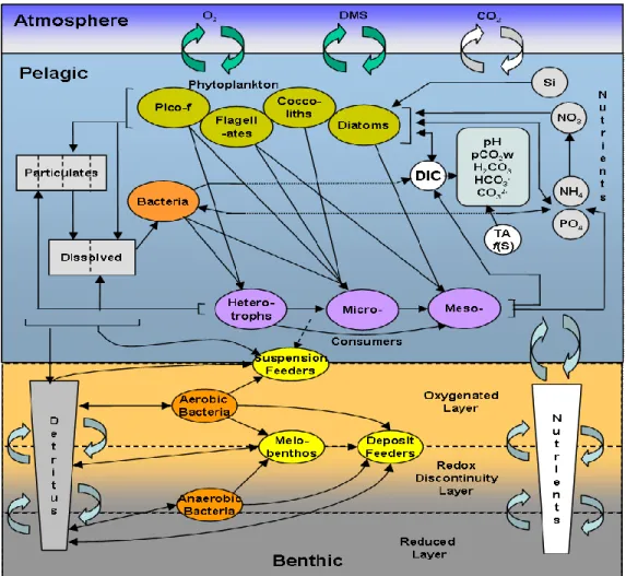
The European Regional Seas Ecosystem Model (ERSEM, Baretta et al., 1995; Blackford et al., 2004) is a biomass and functional group -based biogeochemical model describing the nutrient and carbon cycle within the low trophic levels of the marine ecosystem. Model state variables include living organisms, dissolved nutrients, organic detritus, oxygen and CO2 (Fig.4).
Figure 4. A schematic representation of ERSEM components. N.B. here coccoliths are assumed to be representative of nanophytoplankton
Pelagic living organisms are subdivided in three functional groups describing the planktonic trophic chain: primary producers, consumers and decomposers. Primary producers and consumers are subdivided into 4 and 3 size-based functional types, respectively, while decomposers are modeled through only one functional type. More specifically, the phytoplankton community
16
consists of picophytoplankton, nanoflagellates, dinoflagellates and diatoms. The zooplankton community is divided in mesozooplankton, microzooplankton and heterotrophic nanoflagellates, while decomposers are modeled by one type of heterotrophic bacteria. Functional types belonging to the same group share common process descriptions but different parameterizations.
A key feature of ERSEM is the decoupling between carbon and nutrient dynamics allowing the simulation of variable stoichiometry within the modeled organisms. Chlorophyll is also treated as an independent state variable following the formulation proposed by Geider et al. (1996). Consequently each plankton functional type is modeled throughout up to five state variables describing each cellular component: carbon, nitrogen, phosphorus, silicon, and chlorophyll-a. Primary production is assumed to be not directly dependent on nutrient availability but active DOC (dissolved organic carbon) exudation is accounted in order to re-equilibrate the internal stoichiometry. This mechanism allows for a more accurate description of the nutrient limitation, also ensuring a large production of dissolved organic carbon (DOC) fuelling the bacterial pool. Dissolved organic matter (DOM) is produced by different processes involving phytoplankton, bacteria and zooplankton while its consumption is exclusively regulated by bacteria uptake. DOM is subdivided in a labile and semi-labile component, in order to provide a representation of the range of organic compounds present in the marine DOM and their different degree of degradability. Particulate organic matter (POM) is assumed to be produced by phytoplankton and zooplankton and is divided into a number of size-based categories corresponding to different sedimentation rates. In this way it is possible to realistically simulate the dynamics leading to the carbon export from the surface to the deep ocean.
All together these features make ERSEM a flexible and adaptable model able to simulate, depending on the environmental nutrient concentration, the continuum of trophic pathways proposed by Legendre and Rassoulzadegan (1995), from the classical herbivorous food web (driven by large cell and high nutrient) to the so-called “microbial loop” (Azam et al., 1983) driven by bacteria feeding on DOC (Allen et al., 2002; Polimene et al., 2006, 2007). Thanks to this flexibility ERSEM has been successfully used to investigate different aspects of the marine biogeochemistry in a wide range of ecosystem contexts, from eutrophic coastal environments (Polimene et al., 2007, 2014) to continental shelf seas (Artioli et al., 2012, Blackford et al 2004) and oligotrophic regions (Polimene et al., 2012, Allen et al., 2002). In all the above cited studies, ERSEM has been coupled with a hydrodynamic model providing the physical framework (in terms of diffusive and advective fluxes) necessary to realistically reproduce the marine ecosystem. ERSEM, however, can also be used “standalone” to reproduce idealized systems (see for example
17 Polimene et al., 2006) or laboratory experiments (i.e. batch culture or chemostats) in which physical fluxes (advection and diffusion) can be considered negligible. ERSEM has recently been extended to include the carbonate system giving it a predictive capability for future acidification states (Blackford & Gilbert, 2007; Artioli et al., 2013).
ERSEM is also composed of a benthic module which dynamically simulates nutrient distribution within sediments, organic matter regeneration, bioturbation and bioirrigation along with the dynamics of 7 functional types broadly representing the living compartment of marine sediments. The latter includes suspension feeders (which feed directly from the pelagic system), deposit feeder (which feed on benthic detritus), infaunal predators, epifaunal predators and both aerobic and anaerobic bacteria (Blackford 1997).
1.2.2 Development of ERSEM and a few technical features
Since its first appearance (Baretta et al., 1995) ERSEM was continuously developed. In the pioneering work of Baretta and colleagues (Baretta et al., 1995) the model was used to simulate the ecosystem dynamics of the North Sea. To this purpose, ERSEM was implemented in a set of three dimensional boxes roughly representing the whole North Sea domain. Hydrodynamic fluxes (in the form of daily advective fluxes and diffusion coefficient), temperature and irradiance, were prescribed by an off-line coupling with a General Circulation Model. These physical constrains, along with the depth of each box provided all information specific to the North Sea, whereas the biological/chemical sub-models were constructed not to be site-specific.
Following works (e.g. Baretta-Bekker et al., 1997) improved the physical set-up of the North Sea implementation by rising the number of boxes (up to 130) in which the domain was discretized. Most importantly the decoupling of the carbon assimilation from the nutrient uptake was introduced in the model along with the nutrient uptake dynamics in the bacteria compartment. The improved version of the model was more flexible being able to simulate the full range of food webs, from a system dominated by the microbial loop in the relatively oligotrophic offshore areas to a system dominated by the omnivorous food web in the eutrophic continental coastal area. More recently, ERSEM was further developed by including chlorophyll, as prognostic state variable, and the variable chlorophyll to carbon ratio (Blackford et al., 2004). With all these improvements ERSEM was able to reproduce the main ecosystem dynamics in six highly contrasting sites, with minimal changes in model parameters. Comparison of seasonally depth resolved and integrated properties illustrated that the model produced a wide range of community
18
dynamics and structures that can be plausibly related to variations in mixing, temperature, irradiance and nutrient supply. The model was proposed as a potential basis for an ecosystem-based management tool that may, with appropriate physical representation, be applied over large geographic and temporal scales with utility to both heuristic and predictive studies of the marine lower trophic levels. Latest ERSEM developments include iron dynamics, a more detailed description of bacterial metabolism (Polimene et al., 2006) and the production and fate of climatically active biogases (Polimene et al., 2012).
ERSEM represents the ecosystem as a group of parallel ordinary differential equations (ODEs), solved as an open ended recursive system using continuous simulation techniques (Blackford & Radford, 1995). The essence of the approach is first to define a group of variables which together represent the state of the whole system: its strength is that the rates of all the individual processes over any small time interval may then be defined simply as functions of the state of the system at that time, expressed by the instantaneous values of the state variables modified by external forcing. This enables the large number of individual processes to be conveniently subdivided into groups which may form independent modules linked only by the state variable matrix. This feature of the method facilitates the modular approach that has been adopted for ERSEM.
The choice of state variables was governed by a desire to keep the model as simple as possible without omitting any component which would exert a large influence on the balance of energy flow. The material composition of the state variables and of the transfers which interlink them might be any convenient tracer (e.g. energy). The standard units ensuring compatibility with most measured data sets were used: carbon state variables were represented in mg C m-3 in the pelagic and in benthic pore water region of the model and as mg C m-2 in the benthic layer; similarly nutrients and gases were expressed in mmol m-3 in the pelagic and in benthic pore water but as mmol m-2 in the benthic layer.
The mathematical algorithms used to solve the differential equations were initially included in the software SESAME (Software Environment for the Simulation and Analysis of Marine Ecosystems), written in the programming language Fortran-77 and running on Unix (Ruardij et al, 1995), then in the end of 90s they were directly integrated in ERSEM and re-written by the language “Fortran-90”.
A detailed description of ERSEM-2004, the model version used in this work, is provided in Blackford et al. (2004).
19
2. AIMS OF THIS STUDY
The mechanisms underpinning growth and toxin production in O. cf. ovata, and in dinoflagellates in general, are still far to be fully understood. Often the effects of external environmental factors on O. cf. ovata seem to be different and to depend on the strain: this observed variability in response to external factors could be due to genetic intra-specific variability, or even be due to different methods of detection (and data interpretation) by scientists, but also be caused by different combinations of factors, some of which are unknown. For this reasons, in this work we have decided to operate in an alternative way, focusing on O. cf. ovata single cellular processes in a mechanistic optic.
The principal aim of this thesis was to expand the existing dataset for this species through a new laboratory experiment and to test, by means of numerical simulations, the following hypotheses derived from the analysis of experimental results from several sources:
toxin production consists of a basal (constant) component and an additional term triggered by nutrient stress. The basal component is proportional to the primary production, while the nutrient dependent term is proportional to carbon biomass
concomitantly with the enhanced production of toxins, O. cf. ovata strongly reduces chlorophyll synthesis when stressed by nutrient
O. cf. ovata is able to reduce its metabolism (forming a sort of resting stage) under extreme nutrient limiting condition; the accumulation of cellular carbon and toxins with respect to nutrient and chlorophyll is part of this strategy.
To this end, a newly developed formulation describing toxin compounds production and fate has been implemented in a simplified version of the European Regional Seas Ecosystem Model and used to simulate the experimental dynamics.
An additional goal of the presented work is to improve the range of applicability of a state of the art marine biogeochemical model (ERSEM) by implementing in it an ecological relevant process such as the production of toxic compounds. Finally, with our combined experimental and modelling approach we also meant to highlight current knowledge gaps on the physiology of O. cf. ovata and provide recommendations for future experimental works.
20
3. MATERIALS AND METHODS
In this work we have used the results of two experiments, named Alpha and Beta.
More specifically, Alpha is composed by the union of the two overlapping dataset derived from two experiments previously carried out on an Adriatic O. cf. ovata strain, reported in Pezzolesi et al. (in press) and Pezzolesi et al. (in prep.), since they were identical replicates (also in the obtained results), differing each other only in some conducted analyses. Instead Beta represents the new experiment conducted on the same strain that was arranged for this study: it represents a part of this thesis work, and its data are still unpublished (Pezzolesi et al., in prep.).
3.1 The experiment Beta
3.1.1 Experimental plan
This experiment was conducted on the same O. cf. ovata Adriatic strain OOAB0801 previously used in the experiment Alpha in order to obtain comparable data. This strain has been isolated during a bloom of O. cf. ovata near Bari (Puglia region, Italy) in summer 2008: some single cells of O. cf. ovata were selected from the multi-species field samples using the capillary pipette method (Hoshaw & Rosowski, 1973) and then grown in clonal cultures.
The “Alpha” experiment was conducted using a culture medium derived from an “f/2”, a rich culture medium which is frequently used for the cultivation of marine microalgae (Guillard & Ryther, 1962; Guillard, 1975). In particular a modified “f(N10/P10)” medium was adopted, i.e. an f/2 with concentrations of nitrogen and phosphorus 5-times decreased, with the addition of selenium and without silicon.
In the experiment Beta we decided to grow O. cf. ovata in a limiting condition in terms of nutrients, adopting a “modified f(N150/P150)” medium, i.e. an f/2 with 75-fold decreased nitrogen and phosphorus concentrations, and the same concentration of all the other components, even in this case enriched with selenium and lacking silicon.
This particular medium was prepared using seawater provided by the “Centro Ricerche Marine” (Cesenatico, Emilia Romagna region, Italy) and aged in the dark for a few months in the laboratory. About 10L of seawater with salinity of 35 PSU (measured by a refractometer) were
21 filtered on GF-F glass-microfiber filters (Whatman, porosity 0.7 μm) and then re-filtered on Millipore filters (porosity 0.22 μm) in order to remove bacteria, and were finally sterilized by autoclaving at 120° C for 20 minutes.
All the components of the f/2 medium (less silicon and adding selenium) with a 75-fold decreased quantity of N and P, were appropriately added to the sterile seawater using stock solutions and obtaining a modified f(N150/P150). Chemical compositions of f/2, modified f(N10/P10), and modified f(N150P150) mediums are reported in the Table 2.
Table 2. Chemical composition of different culture mediums: the nutrients are written in red, and the concentrations are expressed in mol/L. Concentrations varying from standard f/2 are highlighted in blue.
The batch cultures were arranged in three sterile 3 L Erlenmeyer flasks, each prepared mixing a medium volume of about 2250 mL and an inoculum of 450 mL containing O. cf. ovata cells obtained from a stock culture (previously acclimated to the new conditions of the experiment for about a week), in order to have a total volume of 2700 mL per flask and a concentration of about 150 cells/mL.
These three identical cultures, named A - B - C, represented the replicates of the Beta experiment, and were grown at the same temperature of 20 ± 1° C in a thermostatic room, under a common PAR (Photosynthetically Active Radiation) of about 125 μE m-2s-1, or 27 W m-2.
22
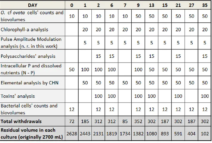
Throughout the course of the experiment several culture aliquots were taken from each replicate in order to perform the various analyses, as reported in Table 3.
Table 3. Samples aliquots taken from each replicate flask with relative target analysis
3.1.2 Cell counts and biovolumes
CELL COUNTS
Culture volumes (10 mL) for counting and cell volume’s estimations were fixed with a few drops of LUGOL, a solution containing iodine and iodide.
To control the cellular growth in cultures several counts have been performed at different days (see Tab. 3): 1 ml of each sample was placed in the counting chamber and then O. cf. ovata cells were counted using an inverted optical microscope Axiovert 100 (Zeiss) at 320 x magnification following the method of Uthermöl (1931). According to this method cells can be counted in each of "a" visual fields of area "b", randomly selected within the total area of the chamber "c", and finally it is possible to calculate the average number of cells per milliliter by the following formula:
23
Alternatively, it is possible to count the cells in each “d” visual field-swiping (with area “e”) taken along the maximum diameter of the chamber, randomly selected by turning the chamber of area “c”, and to calculate the cells’ abundance per mL by the alternative formula:
At the end of the experiment growth curves of each culture were obtained over time, and expressed as cells/mL. Then, considering cells’ counts from the exponential phase (day 1-6), the specific growth rate (μ, expressed as day-1
) was calculated using the following equation:
where and were cell densities values at time (day 6) and (day 1). CELL VOLUMES
Dimensions of O. cf. ovata cells [dorsoventral diameter (DV), Width (W), anteroposterior diameter (AP)] were measured through the software Nis Elements BR 2.20 from the real-time pictures that were taken from the cells using a Digital Sight DSU1 camera (Nikon) connected to the same microscope previously used for the counts (Fig. 5).
24
Minimum 20 measurements for each dimension were taken for each sample. The daily mean cell volumes for each culture have been calculated through the following formula:
where DV = dorsoventral diameter, W = width, = daily mean anteroposterior diameter, n = number of cells per day with known DV and W (from each culture).
This formula calculates the volume of the cells with the assumption of an ellipsoid shape, according to Sun & Liu (2003).
3.1.3 Chlorophyll-a
Chlorophyll-a was measured with a spectrophotometric method.
A volume (10 mL) of sample from each culture (Table 3) was centrifuged at 5000 rpm for 15 minutes at 4° C. Once removed the supernatant, the resulting pellet was re-suspended in 3 mL of 90% acetone, then agitated with a vortex mixer, and stored in the dark for 24 hours in order to allow chlorophyll extraction. After the incubation samples were centrifuged at 3000 rpm for 10 minutes: the supernatant was collected and absorbance was measured at the wavelengths of 750 and 665 nm. The chlorophyll-a was determined according to the following equation (Ritchie, 2006):
( ) [ ( ) ( )]
where:
- A(665s) = the blank corrected absorbance at 665 nm - A(750s) = the blank corrected absorbance at 750 nm
- v = volume of acetone solution used for the extraction (mL) - co = cell path length (cm)
25
3.1.4 Analysis of dissolved inorganic nutrients and organic phosphorus
A volume (50-150 mL) of sample from each culture (Table 3) was filtered on glass-microfiber GF-F filters (Whatman, porosity of 0.7 μm). Both the filtrates (for the inorganic nutrients measurements) and the filters (for the analysis of intracellular phosphorus) were kept frozen at -20° C until further analysis, according to traditional spectrophotometric methods (Strickland & Parsons, 1968).
DISSOLVED INORGANIC NITROGEN
Three different solutions were prepared to perform the analysis:
- “sample” solution: specific volumes (38.5-100 mL) of each filtered culture sample were brought to a final volume of 100 mL by adding synthetic seawater
- “blank” solution, composed exclusively by 100 mL of synthetic seawater
- “standard” solution, prepared with 0.1 mL of standard solution (N-NO3 140 mg/L) and
99.9 mL of synthetic seawater.
In each of the three different solutions 2 mL of concentrated 25% ammonium chloride (m/V) were added.
Then these solutions (sample, blank, standard) were passed for gravity through glass columns filled with granules of metallic coppery cadmium (previously washed with 200 mL of diluted 0.625% ammonium chloride (m/V) and 200 mL of distilled water) in order to reduce any nitrates to nitrites. To avoid collecting any mixed percolate, the first 45 mL of each solution percolated were discarded, while the further 50 mL of each were collected in glass cylinders. In each sample 2 mL of sulfanil-amide 1% (m/V) were added, and after 3 minutes, also 1 mL of 0.1% naphthyl-ethylene-diamine (m/V). After 15 minutes, sample absorbance was measured with the spectrophotometer at 543 nm.
The F factor of each column, which is an index of its efficiency, was calculated:
[ ] ( ) ( )
where [ ] represents the concentration of N-NO3 in the standard solution (0.14 mg/L),
A(543)st is the absorbance of the standard at 543 nm and A(543)b is the absorbance of the blank at the same wavelength.
26
F should have a value between 0.31 (corresponding to 100% of efficiency) and 0.37 (84% of efficiency): higher values indicate that the column need to be re-activated.
Finally it was possible to calculate the nitrates concentrations (expressed as mg/L) in each sample by the formula:
[ ] [ ( ) ( ) ]
where A(543)s represents the absorbance of the sample and V is the original volume of the sample, expressed in mL.
DISSOLVED INORGANIC PHOSPHORUS
The method involves the formation of a phospho-molybdic complex whose concentration is measured colorimetrically at the wavelength of 885 nm.
First a reactive mixture was prepared by mixing four different solutions in a ratio of 2 : 5 : 2 : 1, respectively, i.e. a solution of ammonium molybdate (0.03 g/mL in distilled water), a solution of sulfuric acid (140 mL of 96% acid in 1 L of distilled water), a solution of ascorbic acid (0.054 g/mL in distilled water) and a potassium-antimonile tartrate solution (1.36 mg/mL in distilled water). 50 mL of distilled water for each “blank” solution and 50 mL of each filtered culture sample were placed into graduated 50 mL cylinders. In each cylinder 5 mL of the reactive mixture solution were added, then they were capped and shaken, and finally allowed to stand for 10 minutes, so that the reaction occurs. The resulted compound has a blue color, the intensity of which is proportional to the concentration of phosphates in the starting solution.
Absorbance of the samples were measured at 885 nm using a spectrophotometer, and phosphate concentrations were calculated basing on a calibration curve previously obtained by analyzing several standard solutions of phosphates (KH2PO4), in a range between 0 and 0.456 μg/mL.
ORGANIC PHOSPHORUS
Cells that had been retained on the calcined GF-F filters were digested with 8 mL of a 5% solution of potassium per-sulfate (K2S2O8), as proposed by Menzel & Corwin (1965), and phosphates
released from the organic matter were quantified using the same method as inorganic phosphorus, already mentioned in the previous paragraph.
27
3.1.5 Polysaccharides
To quantify the total polysaccharides produced by O. cf. ovata in our cultures the colorimetric method proposed by Dubois et al. (1956) was followed: it is based on the fact that carbohydrates in the presence of concentrated acids form cyclic compounds called furfurals, which condense with phenols giving colored products that can be analyzed by spectrophotometry.
First it was necessary to extract carbohydrates from the cells, and for this aim we used the method of Myklestad & Haug (1972). A volume (15 mL) of each culture (Table 3) was added to 2 volumes (30 mL) of absolute ethanol in centrifuge tubes, placed at -20° C for 24 hours, and then centrifuged at 12000 rpm for 15 minutes at a temperature of 4° C. Once centrifuged, the supernatant was removed, and 1 mL of 80% sulfuric acid was added to each pellet: the samples thus treated were left to rest at 20° C for 20 hours and then were diluted with 5 mL of distilled water.
After the extraction, polysaccharides were determined by the Phenol Sulfuric Method (Dubois et al., 1956) using glucose as standard (range 0 - 62.5 μg/mL): 2 mL of each sample were mixed to 50 μL of 80% phenol and 5 mL of concentrated sulfuric acid, and were left to rest for 30 minutes at room temperature. Absorbance of the samples was then measured at a wavelength of 543 nm and total polysaccharides’ concentrations were calculated based on the glucose calibration curve.
3.1.6 Elemental analysis (CHN)
Elemental analysis of cellular carbon and nitrogen was performed by using the elemental analyzer Flash 2000, series CHNS/O (Thermo Scientific).
This instrument burns the organic samples, which are contained in tin capsules, in a combustion chamber at 950° C. The pumping of oxygen raises the temperature up to 1800° C and allows a complete combustion of organic matter, resulting in gasification of each element contained in it. The resulting gases, after some reductions, are channeled into a narrow column for gas chromatography, and are finally quantitatively detected through a detector based on the thermal conductivity of some elements: carbon, hydrogen, nitrogen and oxygen.
The 50 mL culture samples (Table 3) were divided in 5 replicates of 10 mL, each of which was filtered through GF-F calcined filters on a small surface area of about 0.3 cm2, then filters were stored at -20° C. Before the analysis they were dried in an oven at 50° C for 10 minutes, then were cut to remove part of the unused filter, and each small filter was placed in a tin capsule.
28
All capsules were directly analyzed, since the presence of the fiber-glass filter in the combustion chamber does not affect the results of the analysis.
A calibration curve obtained using a standard compound, 2,5-Bis (5-tert-butyl-2-benzo-oxazol-2-yl) thiophene (BBOT), was used for quantification of total C and N on each filter. Finally cellular amount were calculated considering culture cell concentration.
3.1.7 Toxins
Toxins were extracted in the laboratory and then analyzed at the Department of Pharmacy, Università Federico II of Naples (Italy), by high resolution liquid chromatography coupled with mass spectrometry (HRLC-MS) (Ciminiello et al., 2011b).
Samples of 100 mL were collected from each replicate on several days (Table 3), and then filtered with GF-F filters. Filters containing the cells were frozen at -80° C, till further treatments in order to extract intra-cellular toxins, while the filtrates containing the extra-cellular toxins were kept frozen at -20° C, until shipment to Naples.
The filters were chopped and placed in centrifuge tubes. Thus a volume (1-1.5 mL, depending on the cells’ concentration at that day) of 50% methanol was added in each tube, then subjected to sonication on ice for 3 minutes (by a Sonicator mod. XL), and finally centrifuged at 12000 rpm for 15 minutes at 4° C (Beckman centrifuge, mod. J2-HS). The resulting supernatant, which contains the toxins extracted from the lysed cells, was collected from each tube: this cycle of extraction and collection was repeated other 2 times, in order to maximize the extraction of toxins from the samples.
Finally the total supernatant of each sample was brought to a final volume of 5 mL by adding 50% methanol, sealed and stored at 4° C until being shipped to Naples.
3.1.8 Cell counts and biovolumes of bacteria
Bacteria abundances in the algal cultures were assessed by direct bacteria counts using epifluorescence microscopy after staining with SYBR gold (Shibata et al., 2006).
More in details, subsample (10 mL) were collected from the algal batch cultures at days 0, 2, 6, 7, 9, 13, 15, 21, 27, and 35. Samples were immediately preserved using 0.2 m pre-filtered formaldehyde (2% final sample concentration), stored in the dark at 4° C until processed within few days. Subsamples (1000 µL or 100 L, depending on growth day) were concentrated onto 0.2
29 µm pore size filters (Anodisc 25 mm, Al2O3) and stained with 100 µL BYBR gold (stock solution
diluted 1:1250). The 100 L subsamples, before being concentrated onto filters were diluted 1:10 with Milli-Q prefiltered sterile water. Filters were incubated in the dark for 15 min and mounted on glass slides with a drop of 50% phosphate buffer saline and 50% glycerol, containing 0.5% ascorbic acid.
Duplicate slides were prepared for each sample. Slides were either counted immediately after preparation or stored at - 20° C for 2-3 days before being counted. Bacterial counts were carried out by epifluorescence microscopy using a Zeiss Axioplan microscope (BP 450-490/FT510/LP520) equipped with an HBO 100 mercury lamp. A minimum of 20-30 randomly chosen fields were viewed at 1000 x magnification.
For each sample a minimum of 20-30 cells were measured for cell volume calculation. Bacteria cells were measured at 1000 x using an image capture system (Nis Elements BR 2.20 software) consisted of a Nikon Digital Sight DSU1 camera connected to the microscope. Cell volume was calculated by assigning simplified geometrical shapes to cells.
3.2 Preparations required for the modelling
3.2.1 Experiments "Alpha" & "Beta" and converting Units of Measure
As already mentioned, the modelling work was based on data, and related interpretations, from the experiments Alpha (Pezzolesi et al., in press; Pezzolesi et al., in prep.) and Beta (this work), since these experiments are almost totally comparable one with the other, and perhaps they are between the most detailed ones ever conducted on O. cf. ovata. These two experiments were conducted using the same Adriatic strain of O. cf. ovata (named OOAB0801), growing it in a medium with the same nitrogen to phosphorus ratio of about 24.4 (thus in phosphorus-limitation), but with a total concentration of nutrients that in the exp. Beta was 15-times lower than in the exp. Alpha. The variables analyzed in the experiment Alpha were exactly the same that have been studied the Beta experiment (except lipids and proteins, not detected in the latter), and also the techniques of analysis were the same.
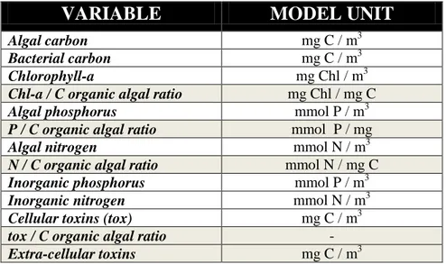
In order to compare modelled and observed variables, experimental values were converted in model units as displayed in Table 4.
30
VARIABLE
MODEL UNIT
Algal carbon mg C / m3
Bacterial carbon mg C / m3
Chlorophyll-a mg Chl / m3
Chl-a / C organic algal ratio mg Chl / mg C
Algal phosphorus mmol P / m3
P / C organic algal ratio mmol P / mg
Algal nitrogen mmol N / m3
N / C organic algal ratio mmol N / mg C
Inorganic phosphorus mmol P / m3
Inorganic nitrogen mmol N / m3
Cellular toxins (tox) mg C / m3
tox / C organic algal ratio -
Extra-cellular toxins mg C / m3
Table 4. ERSEM variables used in this study and relative units. State (prognostic) variables in white fields and secondary (diagnostic) variables in gray fields.
However for diagnostic purposes modelling results reported hereafter are given in mg/L, which is the unit more frequently used in literature in this kind of biological studies.
3.2.2 Data processing
ALGAL CARBON
The first problem we had to face was how to consider the total organic carbon (POC) detected by the CHN analyzer in both the experiments.
The detected POC, in fact, was very high to be considered as only the cellular carbon content of O. cf. ovata. The C:N:P ratios calculated in the last part of the cultures of both the experiments reached values (601:24:1 in the last day of the exp. Alpha, see Table 7 in section 4.2.1) which are well higher than the classical Redfield ratio (106:16:1), that is usually considered the “optimal” internal stoichiometry for marine microalgae (Redfield, 1934, 1958; Tett & Droop, 1988; Hillebrand & Sommer, 1999). Remarkable variations from the Redfield ratio were observed in both field (Geider & La Roche, 2002; Ho et al., 2003) and laboratory (Goldman 1986; John & Flynn, 2000; Klausmeier et al., 2004) studies on marine microalgae, especially when exposed to nutrient limiting conditions. Even considering this, however, the POC:PON:POP ratios detected in our experiments, resulted outside the range of carbon to nutrient ratios described in literature for marine microalgae. Furthermore, also the Chl-a to POC weight ratio reached values (lower limit of 0.0028 and 0.0004 in the exp. Alpha and Beta, respectively) not compatible to the Chl-a:C values observed in cultured marine microalgae usually ranging from 0.1 to 0.01 (Geider 1987, 1993).
31 Finally, such growth of particulate carbon in the last days (21-27-35) of the experiment Alpha, was not justified neither by an increase in cells number, nor by an increase in mean cell volume, and we could say the same for the last part (decaying phase, days 22-35) of the experiment Beta, although to a lesser extent. For all these reasons, we hypothesized that the POC detected by the CHN analyzer in the samples from the last phases of the experiments was biased by the presence of extra-cellular polysaccharidic mucilages, which are usually copiously produced by O. cf. Ovata during the stationary phase (Guerrini et al., 1998; Liu & Buskey, 2000; Pezzolesi et al., in press). This organic matrix is not easily removable with the analytical procedures that we have used (e.g. filtration, see section 3.2.1.) and is likely to have been preserved in the samples when they were analyzed.
The growth curves of O. cf. ovata cellular carbon were, therefore, estimated by correcting the original POC curve in the last phases of the cultures. As already stated, the production of extra-cellular polysaccharides is associated with the stationary phase of the culture. This was also confirmed by the fact that we found a really strong correlation (r > 0.98) between the POC and the total cell volume (obtained by multiplying the number of cells of each day for the mean cell volume of the same day) in the first 15 days of culture of both the experiments (Fig. 23), when the presence of mucilages was still quite low. So the measured POC was a good estimator of algal carbon in the first phase (from exponential to mid stationary) of the cultures. According to this finding, in the second part of the cultures (from day 21 to day 35) the cellular carbon was estimated starting from the total cell volume (measured at each day) and using the linear regressions of the aforementioned correlation between total cell volumes and carbon (see Fig. 22 in section 4.2.3). We used the same regression also to estimate the amount of cellular carbon for the initial day of the cultures (day 0) since direct measurement by CHN were missing.
In summary, the curves of cellular carbon that have been used as experimental guides (and tests) for the model were composed of both the values from CHN measurements and values from the aforementioned data processing (see Fig. 23 in section 4.2.3).
TOXINS
All the different kinds of toxins detected in the experiments (putative palitoxin, ovatoxin-a, -b, -c, -d, -e) were grouped in a single toxic compound. This choice was driven by the fact that all the toxic compounds produced in the cultures were very similar in term of both molecular structure and stoichiometry (129-131 atoms of C, 223-227 atoms of H, 3 atoms of N, 52-54 atoms of O).
32
Furthermore, the relative proportion of each toxic compound resulted to be stable throughout the experiments, as previously observed by Ciminiello et al. (2011b).
Considering the stoichiometric composition of each toxic species and assuming stable proportions between them, both taken from the study of Ciminiello et al. (2011b), we constructed out an “ideal” (average) toxin, with elemental formula C129.66 H224.32 N3 O52.53 : total toxins of
experiments Alpha and Beta were treated as quantities of this “ideal” toxin. Furthermore, in the modelling part of this study only the carbon fraction of this “ideal” toxin was considered as experimental value, since toxins were modelled as a single state variable composed of only carbon.
BACTERIAL CARBON, NITROGEN AND PHOSPHORUS
We estimated the biomass of bacteria starting from bacterial cells’ counts and mean cell volumes. At first was calculated the total volume of bacterial cells from each replicate by multiplying the number of cells for the measured mean volume of a cell (0.433 μm3), and then it was multiplied for a mean value of a carbon content per volume of 145 fg C μm-3, approximated from the works of Fagerbakke et al. (1996) and Steenbergh et al. (2013) on the advice of Prof. Silvana Vanucci: in this way we obtained a rough estimate (with wide margins of error) of the bacterial carbon’s trends in the cultures. Moreover we estimated the bacterial nitrogen and phosphorus, that were calculated starting from carbon through the C:N:P molar ratio of 45:9:1 from Goldman et al. (1987).
3.3 Modelling
3.3.1 General setting of ERSEM and initial conditions
The model used in this work was a simplified version of the pelagic-module of the European Regional Seas Ecosystem Model (ERSEM-2004; Blackford et al., 2004), provided by the Plymouth Marine Laboratory (PML; Plymouth, United Kingdom).
The first part of the modelling work was to enable ERSEM to reproduce a mono-specific batch culture. To this end the model was i) highly simplified, ii) initialized with the data observed (or estimated) at day “0” of the experiments and iii) run under the experimental light and temperature conditions. More specifically:
33 - we considered only one of the four phytoplankton types described in the original model and the bacteria functional type: more specifically, we used the functional group of dinoflagellates and the functional group of heterotrophic pelagic bacteria (P4 and B1 in Blackford et al., 2004, respectively)
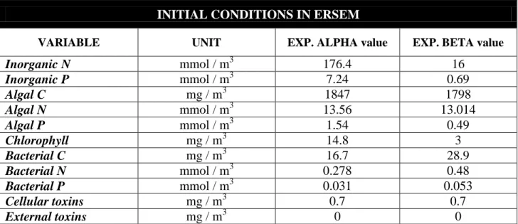
- the model was initialized with nutrient, chlorophyll and biomass concentrations observed (or estimated) at the beginning of each experiment (Table 5)
- the model was run under a 16 - 8 hours light-dark cycle and a constant Photosynthetically Active Radiation (PAR) of 24.35 W m-2 (about 112 μE m-2 s-1) and 27.18 W m-2 (about 125 μE m-2s-1), in order to exactly reproduce the experimental light environment.
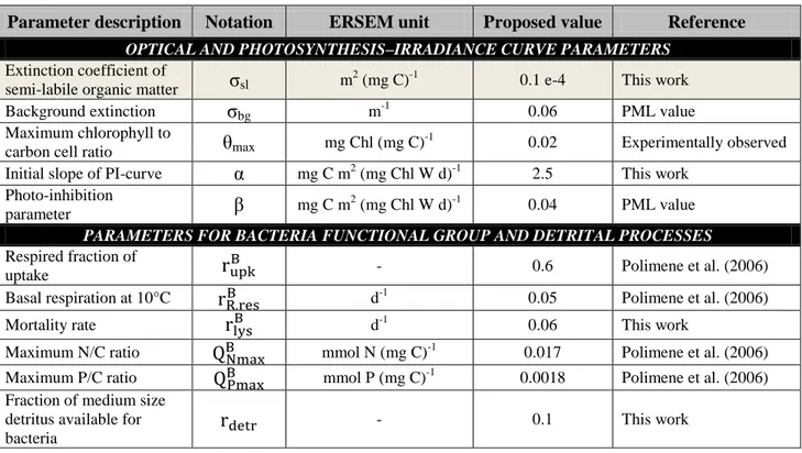
Light extinction in ERSEM is assumed to be dependent only on particles (which are able to absorb and/or scatter the incident radiation). However, in peculiar environments such as a batch culture where dissolved organic matter concentrations can reach extremely high value (as in some eutrophic coastal areas and estuaries) the contribution of the dissolved organic compounds to the extinction of light can be of primary importance. For this reason, and given the high concentration of dissolved polysaccharides observed in the cultures, we have also considered the model state variable “semi-labile DOC” (identifiable with mucilaginous matrices) in the equation describing the attenuation of light in the model (see equation “2” in Blackford et al., 2004).
This step required the creation of the new parameter σsl (reported in Table 6, section 3.3.4): a
light-absorption coefficient for the semi-labile organic matter with a value that is one tenth of the value of the same coefficient for POM.
INITIAL CONDITIONS IN ERSEM
VARIABLE UNIT EXP. ALPHA value EXP. BETA value
Inorganic N mmol / m3 176.4 16 Inorganic P mmol / m3 7.24 0.69 Algal C mg / m3 1847 1798 Algal N mmol / m3 13.56 13.014 Algal P mmol / m3 1.54 0.49 Chlorophyll mg / m3 14.8 3 Bacterial C mg / m3 16.7 28.9 Bacterial N mmol / m3 0.278 0.48 Bacterial P mmol / m3 0.031 0.053 Cellular toxins mg / m3 0.7 0.7 External toxins mg / m3 0 0
Table 5. Some of the initial conditions that were introduced in ERSEM in order to reproduce the exp. Alpha and Beta trends and test our hypothesis. Here are reported only the variables whose values have been changed from the original ones.
34
3.3.2 Modelling toxins production and excretion
Experimental data (see section 4.2.2) of the experiment Alpha showed us that there were significant linear correlations between toxins cellular content (given as toxin to carbon ratio) and both phosphorus to carbon and nitrogen to carbon intra-cellular ratios (r = - 0.85 and r = - 0.79 respectively). Instead for the experiment Beta this correlation was not clear as in the previous case, but only because the P:C and N:C ratios of the alga were very low since the beginning of the experiment, rapidly reaching (and maintaining) values that were on the edge of the lower limit, thereby preventing the display of a linear correlation. On the light of this result, we hypothesized that the toxin production is stimulated by increasing stress conditions of the alga, intending as “stress” the decline in intracellular nutrients to carbon ratios.
O. cf. ovata toxic compounds were modelled through two distinct state variables: tox, indicating cellular toxins, and toxe, indicating extra-cellular toxins, both composed of only carbon, since toxin nitrogen content was considered to be negligible with respect to the total cellular nitrogen budget. Cellular toxin production was assumed to be composed by two additive terms, the first accounting for a constant production assumed to take place under any conditions (in blue field) and the second assumed to be stimulated by intra-cellular nutrient deficiency, or nutrient-stress (in red field): | ( ) ( ) ( )
Where GPP is the gross primary production, A.RESP is the activity respiration, , and
are the minimum, actual and maximum toxin to carbon cellular ratio, respectively, and is
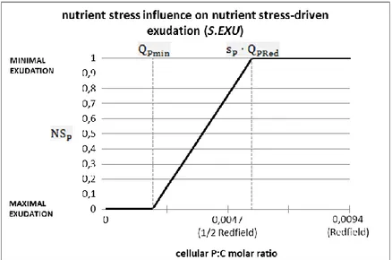
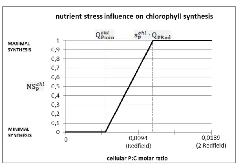
the actual algal biomass (carbon). is the fraction of cellular carbon daily invested in the production of tox during nutrient-stress conditions. NS is the function describing nutrient limitation and is given by:
35 and are determined as:
{ [
( ) ]}
{ [
( ) ]}
where / and / are the actual and minimum phosphorus/nitrogen to carbon cellular ratio, respectively. / are threshold-parameters that determine at what proportion of Redfield ratio (i.e. / ) the cell starts to be nutrient-stressed.
Figure 6 shows with a graphical example how the value changes in function of phosphorus-stress condition of the alga, with a hint about its influence on the nutrient-phosphorus-stress driven exudation (Blackford et al., 2004).
Figure 6. Value trend of the adimensional factor as a function of the intra-cellular P:C molar ratio.
Toxin loss terms were assumed to be composed by lysis, basal respiration and nutrient stress-driven exudation:
|
( )
Where , , are rates of cellular lysis, rest respiration and nutrient stress-driven exudation, respectively (Blackford et al., 2004), and is the actual toxins’ amount in the cells.