Stable laser and upgraded vacuum setup for an experiment with ultracold atoms

(1)

Scuola di Scienze

Corso di Laurea Magistrale in Fisica

STABLE LASER AND UPGRADED

VACUUM SETUP FOR AN

EXPERIMENT WITH

ULTRACOLD ATOMS

Relatore:

Prof. Elisa Ercolessi

Correlatore:

Dott. Francesco Minardi

Presentata da:

Luca Lorenzelli

Sessione III

(2)

Abstract

In questo lavoro ci si propone di descrivere la realizzazione di un sistema laser con cavit´a esterna e di un apparato da ultra-alto-vuoto, che verranno impiegati in un esperimento di miscele di atomi ultrafreddi che utilizza due specie atomiche di bosoni: 87_{Rb e} 41_{K. Speciale attenzione viene rivolta}

verso le caratteristiche dello schema utilizzato e sul sistema di controllo in temperatura, che rendono questo sistema laser particolarmente stabile in frequenza e insensibile alle vibrazioni e variazioni di temperatura. Si sono poi analizzate le propriet´a dei materiali impiegati e delle procedure sperimentali adottate per la realizzazione del nuovo apparato da vuoto, al fine di garantire migliori prestazioni rispetto al sistema attualmente in uso.

(5)

(6)

Introduction

The starting point for the prediction of Bose-Einstein condensation has to be looked for in Bose historic paper of 1924, where he derived Plack’s for-mula by a treatment of black-body radiation as a gas of photons. Einstein argued that what Bose had implied for photons should be true for mate-rial particles as well, and he defined Bose’s derivation of Planck’s formula as an important step towards the quantum theory of ideal gases. In two papers, published soon after that of Bose, Einstein extended Bose’s method to the study of an ideal gas and thereby developed what is now known as Bose-Einstein statistics. The first prediction of Bose-Einstein condensation dates back to the second paper (1925), in which Einstein, considering a gas of non-interacting massive bosons, predicted that, below a certain critical temperature, a finite fraction of the total number of particles would occupy the same lowest-energy single-particle quantum state.

Since that time, the first Bose-Einstein condensate (BEC) was produced 70 years later, thanks to the powerful laser-cooling methods developed in those years. If solids are considered, due to their high atomic density (of or-der 1022cm−3), quantum eﬀects become strong for electrons in metals below the Fermi temperature, which is typically 104_{− 10}5 K. On the other hand, to observe quantum phenomena in dilute atomic gases (the particle density in a Bose-Einstein condensate is typically 1013− 1015 _cm−3_{), temperatures}

lower than 10−6 K are required and this has for such a long time prevented their observation.

13 years after Einstein’s paper, London adopted the phenomenon of Bose-Einstein condensation to develop his Two-Fluid theory for the explana-tion of liquid4He superfluid behaviour at low temperatures. Helium liquids were also the first attractive systems for experimental realization of Bose-Einstein condensates, as the temperatures required for observing quantum phenomena are of order 1 K. On the other hand, due to the strong correla-tions induced by the interaccorrela-tions between4_{He atoms, only a reduced fraction}

(of order 10%) of the total number of atoms can occupy the zero-momentum state, even at absolute zero, with consequent diﬃculties in its detection.

This led to the search for weakly-interacting Bose gases with a higher condensate fraction, and spin-polarized hydrogen was considered a good candidate for this purpose. Indeed, the attractive interaction between two

(7)

hydrogen atoms with their electronic spins aligned was estimated to be so weak that a gas of hydrogen atoms in a magnetic field would be stable against formation of molecules and would thus remain in the gaseous state to ar-bitrary low temperatures. Since hydrogen can’t be laser cooled, cryogenic techniques to force atoms against cold surfaces were employed to realize a precooled state. Nevertheless, interactions of hydrogen with the surface limited the densities achieved in the early experiments and only in 1998 it was possible to realize for the first time a hydrogen atoms Bose-Einstein condensate (the first attempt to realize a BEC with hydrogen atoms was at Massachusetts Institute of Technology MIT where, for the first time, mag-netic techniques for atoms trapping were developed). Besides laser cooling techniques, a peculiar process that allow to achieve the low temperatures and high densities required for the onset of Bose-Einstein condensation, is an evaporative cooling stage of magnetically trapped gases, in which the more energetic atoms are removed from the trap, thereby cooling the remainings. Finally, as a consequence of the progress made in laser cooling of alkali atoms and evaporative cooling techniques, the first gaseous Bose-Einstein conden-sates for rubidium, sodium and lithium were realized in 1995. A peculiar feature of this kind of systems is the possibility to manipulate them by the use of lasers and magnetic fields, that allow for example to study their be-haviour, while varying the interactions between atoms exploiting Feshback resonances.

The reason why the physics of ultracold atoms is still nowadays an im-portant field of theoretical and experimental research, is because ultracold gases loaded into optical lattices can provide highly controlled quantum sys-tems for simulations of other quantum syssys-tems. Bose-Einstein condensates give the unique opportunity for exploring quantum phenomena on a macro-scopic scale and ultracold atoms in optical lattices can be used for condensed matter physics simulations, as their behaviour is similar to that of electrons in solids, where the real periodic potential formed by the ions is replaced by an artificial crystal potential formed by an optical lattice. Indeed, although these systems are quite diﬀerent in the absolute energy and length scales, one can use ultracold atoms to implement the model Hamiltonians that have long been studied in the context of strongly correlated electronic systems. Furthermore, they constitute a clean system without any lattice defect and show a high scalability, in that, with such systems, it is possible to tune the lattice parameters over a wide range, with a high degree of controllabil-ity. Besides the quantum simulation aspect, recent experiments on ultracold atoms in optical lattices (such as single-site resolution imaging techniques), have opened the door to quantum information processing, due to their long coherence times.

Eventually, two basic, but at the same time fundamental aspects con-cerning ultracold atoms experiments are the laser and vacuum techniques. Indeed, these experiments require an extremely high degree of vacuum, in

(8)

CONTENTS 7 the range of ultra-high-vacuum (i.e. pressures of the order of 10−11 mbar), to prevent thermalization between the atoms and the walls of the experi-mental apparatus, through collisions with the particles of the residual gas. Such extremely low values for the pressure involves a careful choice of the building materials, as well as the requirement to optimize the experimental techniques for the realization of vacuum systems. In the same way, laser cooling is of crucial importance and the great number of lasers involved in these experiments, as well as the complexity of the optical elements setup, imply inexpensive ways to realize compact laser systems with high reliability, expecially as far as their wavelength stability, tunability and output power are concerned. It is for this reason that so basic experimental aspects, like vacuum and laser techniques, are at the same time so important in ultracold atoms experiments and need a continuous research aimed to improve their performance.

The purpose of this thesis is to present the development of a partic-ularly stable external-cavity diode laser that uses an interference filter as wavelength selector and of an upgraded vacuum system, that will be em-ployed in an experiment with ultracold atoms that involves two diﬀerent species of bosonic alkali atoms: 87Rb and41K. The systems described in the present work involve new and advanced techniques in their respective fields. They are aimed to the specific necessities of a laser for cooling 87_{Rb atoms,}

that has to be particularly stable against mechanical vibrations and thermal fluctuations, in order to ensure the best performance. The aged vacuum ap-paratus currently in use needs to be improved with a new one, that should guarantee a better optical access for laser interaction with atoms and the use of high-intensity trapping magnetic fields, without residual magnetiza-tion eﬀects. The introducmagnetiza-tion given in this thesis will concern an upgraded vacuum system, that makes use of advanced materials for ultra-high-vacuum (UHV) technology, so that the lowest level of residual gas particles released from material surfaces and the minimization of mechanical stresses due to thermal strains, at the interface of diﬀerent materials, can be achieved.

As far as the organization of this work is concerned, chapter 1 gives an introduction to the quantitative description of Bose-Einstein condensation in dilute gases. We will deal first with the ideal case, while interactions will be introduced in sections 1.3 and 1.4, where the Gross-Pitaevskii equation and the Thomas-Fermi approximation will be presented.

Chapters 2 and 3 are devoted to the description of my experimental work at the European Laboratory for Non-Linear Spectroscopy (LENS), at the University of Florence. Sections 2.1 and 2.2 introduce to the the-ory of interference-filter-stabilized external-cavity diode lasers and section 2.3 gives the details of our system, that provides advantages for what con-cerns the wavelength stability and the optical feedback optimization, with respect to the common grating-stabilized diode lasers previously used. Sec-tion 2.4 gives then the detailed descripSec-tion of the feedback system for the

(9)

diode’s temperature control, that includes the software implementation of LabVIEW projects on the Field Programmable Gate Array (FPGA) chip and Real-Time processor of a National Instruments device. Finally, in sec-tion 2.5, we will report and discuss the results attained with our system.

Chapter 3 is focussed on the realization of an ultra-high-vacuum (UHV) system: section 3.1 introduces the basic concepts that concern vacuum tech-nology. Section 3.2 describes the setup of our system, with particular atten-tion to the behaviour of materials in UHV and points out the main features that make titanium vacuum chambers (like the one we used) particularly suitable for UHV applications. Eventually, in subsection 3.2.4 and section 3.3, we will analyze the results obtained from the characterization of our system and give hints aimed to improve the vacuum setup experimental techniques developed in this work.

(10)

Chapter 1

Bose-Einstein condensation

1.1 Bose - Einstein condensation in non

interact-ing systems

Consider an ideal Bose gas with a fixed number of particles N, i.e. subject to the constraint

N =

+_�∞ ε=0

nε (1.1)

The Bose-Einstein statistics for the mean occupation number of single-particle states is < nε> = 1 e (ε−µ) kBT _{− 1} (1.2) which means that we must have µ < l ε, ∀ε (otherwise unphysical negative populations may result). For µ < εmin = 0, all values of (ε− µ)

are positive and the behaviour of all < nε> is nonsingular.

In the high temperature limit, the quantum Bose-Einstein and Fermi-Dirac statistics (< nε >= 1

e

(ε−µ) kBT _∓1

) tend to behave in the same classi-cal fashion, described by the Maxwell-Boltzmann statistics (< nε >M.B.=

e

(ε−µ) kBT _).

This is equivalent to the non-degeneration condition e

(ε−µ)

kBT _{>> 1} _(1.3)

which physical meaning is that the probability of double occupance is negligible for any of the single-particle levels ε

< nε> << 1 ∀ε (1.4)

(11)

For bosons, condition 1.3 implies that µ, the chemical potential of the system, must be negative and large in magnitude. This means that the fugacity z≡ ekBTµ _{of the system must be much smaller than unity.}

One can see [2] that this is equivalent to the requirement

nλ3 << 1 (1.5)

where n = N_V is the total density of particles and λ = h

(2πmkBT ) 1

2 is the

thermal deBroglie wavelength.

On the other hand, when the temperature tends to zero, µ becomes equal to the lowest value of ε. In this regime the non-degeneration condi-tion 1.3 breaks down and the occupancy of the single-particle ground-state ε = 0 becomes infinitely high, leading to the phenomenon of Bose-Einstein condensation.

A statistical treatment of an ideal Bose gas provides the thermodynamic expressions P V kBT ≡ lnZ(z, V, T ) = − � ε ln(1− ze−βε) (1.6) N _≡� ε < nε>= � ε 1 z−1_eβε_{− 1} (1.7)

with Z(z, V, T ) the grand partition function of the system. If we consider the thermodynamic limit (N, V → ∞;N

V = n = const) ,

the spectrum of the single-particle states is almost a continuum one and the summations may be replaced by integrations, according to

1 V � ε → 2π h3(2m) 3 2 � _∞ 0 ε 1 2dε (1.8) where g(ε)dε � V h3(2m) 3

2ε12dε is the number of single-particle states in

the infinitesimal range from ε to ε + dε.

We observe that, taking the thermodynamic limit, we are giving a weight zero to the ground energy level ε = 0. As in a quantum mechanical treatment we must give a statistical weight unity to each nondegenerate single-particle state in the system, it is advisable to take this particular state out of the sum before carrying out the integration. We thus obtain the general expressions:

P kBT =−2π h3(2m) 3 2 � _∞ 0 ε 1 2ln(1− ze−βε)dε− 1 Vln(1− z) (1.9) N V = 2π h3(2m) 3 2 � _∞ 0 ε12dε z−1_eβε_{− 1}+ 1 V z 1− z (1.10)

(12)

1.1. NON INTERACTING SYSTEMS 11 Since, from equation 1.2: _1−zz = N0 (number of particles in the ground

state ε = 0) and hence z = N0

N0+1, the last term in equation 1.9 is equal to

1

Vln[(N0+ 1)−1], and we can neglect it for all values of z.

Now, substituting βε = x and taking into account that _V1 ₁_−zz = N0

V , we

can rewrite expressions 1.9 and 1.10 in terms of Bose-Einstein functions, defined by: gν(z) = 1 Γ(ν) � _∞ 0 xν−1dx z−1_ex_{− 1} (1.11) where Γ(ν) =�₀∞e−xxν−1dx. Thus: P kBT =−2π(2mkBT ) 3 2 h3 � _∞ 0 x 1 2ln(1− ze−x)dx = 1 λ3g52(z) (1.12) N_{− N}0 V = 2π(2mkBT ) 3 2 h3 � _∞ 0 x12dx z−1_ex_{− 1} = 1 λ3g3₂(z) (1.13)

This last equation determines the value of the fugacity z.

From these expressions we can calculate other thermodynamic quanti-ties, such as the internal energy

U ≡ −( ∂ ∂βlnZ)z,V = kBT 2� ∂ ∂T( P V kBT )� z,V = kBT 2_{V g} 5 2(z) � _d dT( 1 λ3) � = 3 2kBT V λ3g52(z) (1.14) and the specific heat of the gas

CV N kB ≡ 1 N kB �_∂U ∂T � N,V = 3 2 � _∂ ∂T � _{P V} N kB �� (1.15) From these expressions we can determine the equation of state for the system: P = 2 3 �_U V � (1.16) Let us now consider one first step far from the classical limit.

When z << 1, we can expand Bose-Einstein functions as gν(z) = z +z

2

2ν +

z3

3ν + ... (1.17)

If we neglect N0 in comparison with N and inverte the series in 1.13, we

obtain an expansion for z in powers of nλ3_{. Then, subtituting this into the}

(13)

P V N kBT = +∞ � l=1 al �_λ3 v �l−1 (1.18) where v ≡ 1

n is the volume per particle and al are the virial coeﬃcients

of the system.

The specific heat is expressed as CV N kB = 3 2 +∞_� l=1 5_{− 3l} 2 al �_λ3 v �l−1 (1.19) We observe that, as T _{→ ∞ (and hence λ → 0), both the pressure and} the specific heat of the gas approach their classical values: nkBT and 3₂N kB,

respectively.

We are now going to consider another situation, in which z increases and assumes values close to unity, so that expansion 1.17 is no longer valid.

We see that the term ₍₁_−z)Vz (which is identically equal to N0

V , N0 being

the number of particles in the ground state ε = 0 ) can become a significant fraction of the quantity N_V.

The physical meaning of this result is that a macroscopic fraction of particles occupy the quantum single-particle state ε = 0.

Expansions such as 1.18 and 1.19 do not remain useful and we have to work with the general thermodynamic expressions 1.12, 1.13 and 1.14. From 1.13 we can express the number of particles in the excited states

Ne= V (2πmkBT ) 3 2 h3 g32(z) (1.20) As T _{→ 0, z =} N0 N0+1 → N N +1 � 1 and, as g3₂(z) is a monotonically

increasing function of z (its largest value being g3

2(1)≡ ζ(

3

2)� 2, 612), the

total number of particles inl the excited states is bounded by

Ne≤ V (2πmkBT ) 3 2 h3 ζ( 3 2) (1.21)

As long as the actual number of particles in the system is less than this limiting value, nearly all the particles in the system are distributed over the excited states and the precise value of z is determined by equation 1.20. However, for a higher number of atoms, the exiding ones will be pushed into the ground state ε = 0:

N0 = N − � V(2πmkBT ) 3 2 h3 ζ( 3 2) � (1.22) Hence, the condition for the onset of Bose-Einstein condensation is

(14)

1.2. THE IDEAL TRAPPED GAS 13 N > V T32(2πmkB) 3 2 h3 ζ( 3 2) (1.23)

or, if we hold N and V constant and vary T T < TC = h2 2πmkB � _N V ζ(3₂) �3 2 (1.24) TC is a characteristic temperature that depends on the mass of the

par-ticles m and on the density N_V of the system. One characteristic feature is that, at TC, the thermal wavelength λ = h

(2πmkBT ) 1

2 is comparable to the

interparticle spacing.

1.2 The ideal trapped gas

Consider a vapour of nearly non-interacting atoms. The first step needed for its cooling consists of a laser cooling with three counter propagating laser beams, tuned just below the resonant frequency of the atoms in the trap (detuned towards red). With this configuration, moving atoms are Doppler shifted on resonance to the laser beam that is propagating opposite to their velocity, while atoms at rest are just oﬀ resonance and so rarely absorb a photon. Those atoms which are on resonance, then reemit photons, with a resulting net momentum kick opposite to the direction of their motion. The final result is an optical molasses that slows the atoms. This cooling method is constrained by the so called recoil limit, in which the atoms have a minimum momentum of the same order of magnitude of the momentum of the photons emploied to cool the gas. This gives a limiting temperature of _2mc(¯hω)2_k2_B � 1µK , where ω is the frequency of the spectral line used for

cooling and m is the mass of an atom.

The following step of the cooling process is an anisotropic harmonic oscillator potential trapping the atoms near the center of the magnetic trap:

V (r) = 1 2m(ω

2

xx2+ ω2yy2+ ωz2z2) (1.25)

(In this situation the lasers are oﬀ and the trapping frequencies ωi are

controlled by an applied magnetic field). Then, the highest energy atoms are removed by decreasing the trap barrier potential and the remainings are hence cooled by evaporation.

If the atoms in the trap are not interacting, the total Hamiltonian of the system is the sum of single-particle Hamiltonians, whose eigenvalues are the energy levels for each atom

εlxlylz = ¯hωxlx+ ¯hωyly+ ¯hωzlz+

1

(15)

where li = 0, 1, 2, ...,∞ are the quantum numbers of the harmonic

os-cillator. Assuming a grand-canonical theory, we have, for bosons in the trap, the thermodynamic potential Π (determined from the grand canonical partition function) Π(µ, T ) =₋(kBT ) 4 2(¯hω0)3 � _∞ 0 x2ln(1_{− e}−xeβµ)dx = (kBT ) 4 (¯hω0)3 g4(z) (1.27)

that allows to evaluate the avarage number of atoms in the excited states of the trap N (µ, T ) =�∂Π ∂µ � T = �_k_B_T ¯hω0 �3 g3(z) (1.28)

For a fixed number N of trapped atoms, the chemical potential monoton-ically increases as the temperature is lowered, until Bose-Einstein conden-sation sets up when the chemical potential reaches its highest value µ = 0, at the critical temperature

kBTC ¯ hω0 =� N ζ(3) �1 3 �� N 1, 202 �1 3 (1.29) Observed critical temperatures are about few hundreds nK.

For T < TC we can determine the number of atoms in the excited states

by separating the term representing the population of the ground state of the harmonic trap, in the expression for the total number of particles

N _{− N}0 = � lx,ly,lz�=0 � 1 eεlxlylzkBT _{− 1} � (1.30) For N >> 1, the energy levels spacing ¯hω0 becomes much smaller then

the typical excitation energy kBT of the system and the previous summation

can be replaced by integration N_{− N}0= � _d3_�n e(kBT¯h �ω·�n)_{− 1} = ζ(3)�kBT ¯ hω0 �3 (1.31) or equivalently Nexcited N = ζ(3) N �_k_B_T ¯hω0 �3 =� T TC �3 (1.32) Here ζ(n) = �∞_k=1k−n is the Riemann Zeta function and �ω, �n collect the trapping frequencies and quantum numbers along each direction. At T = TC there is a zero population in the ground state and from expression

1.31 we recover 1.29, that defines the critical temperature TC. So, below TC,

the fraction of atoms that condense into the ground state of the harmonic trap is:

(16)

1.2. THE IDEAL TRAPPED GAS 15 N0 N = 1− � _T TC �3 (1.33) The result is that, in the thermodynamic limit, a non zero fraction of the atoms occupy the ground state for T < TC, while the occupancy fraction of

each excited state is zero.

Detection of Bose-Einstein condensation is usually carried out by mea-suring the momentum distribution of the ultracold gas by a time of flight experiment. In this description we consider as time t = 0 the time at which the magnetic field is turned oﬀ and the trapping potential goes to zero. The atomic cloud can thus expand according to the momentum distribution the atoms had in the harmonic trap, for an allowed time of about 100ms. We no-tice that at such low temperatures the speed of the atoms is a few millimeters per second and so the cloud expands to a few hundred microns in this period of time. The cloud is then illuminated with a resonant laser pulse, leaving a shadow on a CCD in the image plane of the optics. The size and shape of the light intensity pattern directly measures the momentum distribution the atoms had in the trap at t = 0. The expanding cloud can be divided into two components, the N0 atoms that had been Bose condensed into the ground

state, whose wavefunction is the product of the single-particle ground state eigenfunctions in the harmonic trap (with nx= ny = nz= 0):

Ψ0 = � i ψ0(�ri) (1.34) with ψ0(�r) = � mω0 π¯h �3 4

e−mω02¯h (ωxx2+ωyy2+ωzz2), and the remainings N− N₀

atoms that were in the excited states of the harmonic oscillator potential. The Bose-condensed atoms had smaller momenta than the atoms that were in the excited states and, after time t, the quantum evolution of the ground state has the spatial number density distribution:

n0(�r, t) = N0|Ψ0(�r, t)|2= N0 π32 � j=x,y,z � 1 aj � 1 + ω2_jt2e −_a2 r2j j(1+ω2jt2) � (1.35) aj = � ¯ h

mωj is the linear spatial extention of the ground state

wavefunc-tion along cartesian direcwavefunc-tion j, while the mean width of the noncondensed atomic distribution is ajthermal =

� kBT mω2 j = aj �_k BT mωj.

The atoms that are not condensed into the ground state can be treated semiclassically: one assumes a classical position-momentum distribution and a quantum Bose-Einstein statistics for their occupancy.

f (�r, �p, 0) = 1

e[2mkBTp2 +kBTm (ωx2x2+ωy2y2+ω2zz2)]−_kBTµ _{− 1}

(17)

We conclude this section observing that, at early times (ωjt << 1),

both the condensed and the excited spatial distributions are anisotropic, due to the anisotropic trapping potential, while, during further expansion, the atoms from the excited states form a spherically symmetric cloud, because of the isotropic momentum dependence of the t = 0 distribution function 1.36. By contrast, for the atoms that were condensed into the ground state, the direction that has the largest ωj is quantum mechanically squeezed the

most, at t = 0. So, according to the uncertainty principle, it expands the fastest.

1.3 The interacting Bose gas at T = 0: the Gross

−

P itaevskii equation

Let us now introduce interactions between particles and consider N inter-acting atoms, confined in an external magnetic trap potential, that can be approximated by an anisotropic harmonic oscillator potential of the form 1.25, as before.

In the second quantization formalism, the total Hamiltonian of the sys-tem is ˆ H = � d3�r ˆΨ†(�r)�₋¯h 2 2m∇ 2_+V trap � ˆ Ψ(�r)+1 2 � d3�rd3�r�Ψˆ†(�r) ˆΨ†(�r�)[Vint(�r−�r � )] ˆΨ(�r) ˆΨ(�r�) (1.37)

The first term is a single-particle one, while the second is a two body term, representing atom-atom interactions.

ˆ

Ψ†(�r), ˆΨ(�r) are bosonic field operators, acting in the Fock space

F =_⊗∞_n=1Hn, that create and destroy one particle at position �r,

respec-tively. They can be expressed in terms of single-particle wavefunctions un(�r)

as ˆ Ψ†(�r) = ∞ � n=1 a†_nu∗_n(�r) (1.38) ˆ Ψ(�r) = ∞ � n=1 anun(�r) (1.39)

The starting point for the theory we are going to develop is the time-dependent Schr¨oedinger equation, written, in Heisenberg formalism, as:

[ ˆΨ(�r, t), ˆH] = i¯h∂

∂tΨ(�r, t) = E ˆˆ Ψ(�r, t) (1.40) Here ˆH is the Hamiltonian of the system and E its total energy.

(18)

1.3. THE INTERACTING BOSE GAS AT T = 0 17 Now we try to solve the problem of determining the temporal evolution of the system with a variational method. The destruction field operator [ ˆΨ(�r, t)] can be decomposed into two terms:

ˆ

Ψ(�r, t) = Ψ0(�r, t) + δ ˆΨ(�r, t) (1.41)

where δ ˆΨ(�r, t) represents a small perturbation and Ψ0(�r, t) =�Ψ0| ˆΨ(�r, t)|Ψ0�

is the ground state expectation value for the field operator ˆΨ(�r, t). We notice that, as the condensate fraction of the system is not invariant under U (1), the number of condensed particles is not conserved and hence Ψ0(�r, t)�= 0.

At low energies, a fairly accurate description is provided by approximating interactions by an eﬀective contact potential:

Vint(�r− �r

�

) = u0δ(�r− �r

�

) (1.42)

where u0 is the interaction constant. This is just the case for ultracold

gases, since the kinetic energy and the density of the particles are small. Approximating ˆΨ(�r, t) with its ground state mean value Ψ0(�r, t) and

using assumption 1.42 in equation 1.40, gives the Gross-Pitaevskii equation (GPE) i¯h∂ ∂tΨ0(�r, t) = � −¯h 2_∇2 2m + Vtrap(�r) + u0|Ψ0(�r, t)| 2�_Ψ 0(�r, t) (1.43)

to which corresponds the Gross-Pitaevskii energy functional

E[Ψ0] = � d3�r�Ψ∗₀(�r, t) ˆHΨ0(�r, t) � = � d3�r �_¯_h2 2m|�∇Ψ0(�r, t)| 2_+V trap(�r)|Ψ0(�r, t)|2+ 1 2u0|Ψ0(�r, t)| 4� (1.44) This represents the mean field energy in terms of the macroscopic quan-tum state wavefunction Ψ0(�r, t), where Ψ∗0(�r)Ψ0(�r) =|Ψ0(�r, t)|2is the

macro-scopic ground-state number density n0(�r).

We can now minimize the functional E[Ψ] with respect to Ψ∗, taking into account the constraint that the total number of atoms in the system is constant N = � n(�r)d3�r = � |Ψ(�r)|2d3�r (1.45)

By introducing the Lagrange multiplier µ (i.e. the chemical potential of the system) and setting δE_{− µδN = 0, the Gross-Pitaevskii equation takes} the form: ¯ h2 2m∇ 2_Ψ 0(�r)2+ Vtrap(�r)Ψ0(�r, t) + u0|Ψ0(�r)|2Ψ(�r) = µΨ(�r) (1.46)

(19)

This expression is quite appropriate for describing the zero-temperature nonuniform Bose gas when the range of the interaction between atoms is much smaller than the avarage interparticle spacing. We can notice that, when interactions are included, the equation describing the condensate is in the form of a single-particle Schr¨oedinger equation with an additional non-linear term proportional to u0|Ψ(�r)|2, that provides the mean field coupling

of one particle to all the remainings.

In order to determine the mean field ground-state energy, one solves the Gross-Pitaevskii equation 1.46 for Ψ(�r) and uses the solution to evaluate the energy functional 1.44.

We are going now to analyze the various situations corresponding to the diﬀerent kinds of interactions between particles. The coupling constant u0 = 4πa¯h

2

m depends on the scattering length a. If a is positive, the

in-teraction is repulsive, while if a is negative the inin-teraction is attractive. When a = 0, the solution of equation 1.46 is the noninteracting ground-state wavefunction Ψ(�r) =√N φ(�r), while in the repulsive case (a > 0), if N is suﬃciently large, the GPE can be analitically solved employing the Thomas-Fermi approximation. By contrast, in the case of attractive con-densates (a < 0), only numerical and variational analysis are available.

1.4 Ground state of a repulsive condensate: the

T homas

_{− F ermi approximation}

The Thomas-Fermi regime is a useful assumption that allows to derive an expression for the system ground state wavefunction when the atomic clouds are suﬃciently large. This statement is equivalent to the condition

N|a|

aho >> 1, where the dimensionless parameter

N|a|

aho controls the strength of

the interaction term (aho = (axayaz)

1

3 represents the average linear size of

the unperturbed harmonic oscillator ground state and a > 0 is the scattering length, that characterizes the interaction between atoms). If this situation is satisfied, the kinetic energy term−¯h_2m2∇2 is much smaller than the interaction one, and the GPE can be written as:

[Vtrap(�r) + u0|Ψ(�r)|2]Ψ(�r) = µΨ(�r) (1.47)

leading to the Thomas-Fermi solution:

Ψ0(�r)�

�

(µ_{− V}trap(�r))

u0

(1.48) that gives for the density of particles:

(20)

1.4. GROUND STATE OF A REPULSIVE CONDENSATE 19 We notice that, as the solution must be positive, the boundary of the cloud is given by the condition:

Vtrap(�r) = µ (1.50)

Hence, solution 1.49 is diﬀerent from zero in the region defined by µ > Vtrap(�r), while |Ψ0(�r)|2 = 0 otherwise. For a harmonic trap, the density

distribution is an inverted parabola, whose maximum coincides with the potential minimum.

Taking into account the boundary condition 1.50 and the expression of the harmonic trap potential V (�r) = ₂1m(ω_x2x2+ ω_y2y2+ ω2_zz2), we can deduce an expression for the cloud extention along the three cartesian directions. It can be found that:

Ri = � 2µ mω2 i (1.51) with i = x, y, z. Besides, the normalization condition on Ψ(�r)

�

d3�rnT−F = N (1.52)

yelds the following relation between the chemical potential µ and the total number of bosons N

µ = 1 2¯hωho(

15N a aho

)25 (1.53)

and finally, by combining 1.52 and 1.51, we obtain the spatial extention of the condensate in the Thomas-Fermi regime, expressed in terms of the harmonic trap characteristic length:

RT−F = aho �_{15N a} aho �1 5 (1.54) Since µ = _∂N∂E and µ _{∝ N}25, the total energy of the condensate in this

limit is

E = 5

7µN (1.55)

The eﬀect of repulsive interactions between bosons is therefore to expand the size of the condensate, making the anisotropy of the system and time-of flight distributions more anisotropic than in the noninteracting case. In fact, in time-of flight measurements, the repulsive interactions result in higher velocities in directions that were more confined in the trap.

The Thomas-Fermi length 1.54 indicates that the dependency of the condensate extention on the number of atoms N . This is a characteristic feature due to the introduction of interactions.

(21)

We are now going to make some observations concerning the attractive case. This situation corresponds to a negative scattering length a < 0. The presence of attractive forces between atoms makes the condensate to increase its density, thus reducing the extention, until equilibrium is reached through the balance between the compressing interaction term and the kinetic energy one, which, by contrast, tends to expand the condensate. Anyway, there exists a critical value for the number of atoms in the condensate, NC, beyond

which the kinetic pressure can’t contrast the attractive interaction and the condensate collapses. However, in general, a long-lived atomic condensate exists for small negative values of the parameter _aN a

ho. This implies that the

kinetic energy term in the Gross-Pitaevskii equation 1.46 can’t be neglected with respect to the interaction term and the Thomas-Fermi approximation is no longer valid. Now, the system can’t be treated analitically, but the study of its ground-state and the critical number NC can be carried out

(22)

Chapter 2

A stable external-cavity

diode laser to cool

87

Rb atoms

We will present here our laser setup, giving first an introduction about diode lasers and external-cavity diode lasers with an interference filter as wavelength selector. Then, we will report the details for the build up of the external cavity, the interference filter and the electronics and software developement for the feedback system that controls the wavelength stability. Eventually, we will compare the results that we obtained with and without the external cavity, in order to demonstrate the advantages given by this latter configuration.

2.1 Introduction

Dealing with atomic physics experiments, the basic requirement is to have an interaction between atoms and coherent light. Diode lasers were used for the first time in this field of physics in the early 80’s and, since that moment, their performances were rapidly improved and there has been a great deal of research about these systems. The main characteristics that have made diode lasers so important are their high reliability and tunability, but also the fact that they are inexpensive sources of light, so that every laboratory can aﬀord them. The first employed diode lasers were simple free running devices, without feedback, mainly used for low resolution spec-troscopy. Nevertheless, since the 90’s, they have been steadily improved in power as well as in wavelength coverage, while decreasing costs. Feedback systems were also developed, allowing narrower linewidths (of the order of few hundreds kHz) and more stable amplitudes and frequencies.

The wavelength control techniques have made possible advanced applica-tions for standard commercial diode lasers in atomic physics and we are now going to examine the mainly ones. Optical pumping consists of cyclically pump electrons, bound within an atom or molecule, to a defined quantum

(23)

state. Considering an alkaline atom, for which only one electron belongs to the outermost shell, a coherent two level optical pumping means that the electron is coherently pumped to a single hyperfine sublevel and the atom is said to be oriented in that particular sublevel. The optical pumping has a cyclic nature, so that the electron experiences repeated transitions between upper and lower state sublevels and the orientation of the atom is deter-mined by the polarization and frequency of the laser light, as well as the linewidth and transition probability of the absorbing transition.

Diode lasers are also employed in applications using fast frequency mod-ulation, because it is particularly easy to modulate their amplitude and fre-quency very fast (the modulation response for common diode lasers extends out to a few GHz) and through large ranges. This can be achieved modulat-ing the injection current of the diode laser, which produces both amplitude (AM) and frequency (FM) modulation. The injection current modulation spreads out the diode laser’s spectrum into many discrete sidebands and this eﬀect increases with the strength of the modulation. The modula-tion sidebands method finds many applicamodula-tions, as it allows to increase the signal-to-noise ratio and thus to detect atomic or molecular resonances with high sensitivity. For molecular species spectroscopy, also, ”two-tone” mod-ulation methods (modmod-ulations at two diﬀerent frequencies) were developed and the modulation into sidebands is generally useful in atomic and molec-ular physics experiments were numerous frequencies are required. Further-more, diode lasers have the unique capability to sweep the laser frequency extremely rapidly in a controlled manner, by an high speed switching, or pulse. This jumping of the output frequency permits to reduce the num-ber of lasers needed in optical pumping experiments; indeed, for example, it is possible to optical pump some kind of alkaline atoms into a specific magnetic sublevel using only one single laser [4]. The frequency modulation capability is also succesfully used to slow down and stop atomic beams, as well as to rapidly probe atomic velocity distributions. Their performances are limited by the broadness of the laser linewidth, but they can be seri-ously improved by an external cavity that stabilizes the laser and narrows its linewidth, with a resulting increase in the number of slowed atoms and a decrease in the spread of the velocity distribution. As mentioned above, feedback-stabilized diode lasers are unique, in that thay provide simple and inexpensive sources of narrowband tunable and stable amplitude light, which involves very good signal-to-noise ratios and make them suitable for high res-olution spectroscopy. In fact, with this high precision measurement systems, atomic transition spectra can be detected, with spectral linewidths only lim-ited by the natural linewidth of the transition and not by that of the laser (which can be lower than 100 kHz).

For us, the most important area concerning stabilized diode lasers is laser cooling and trapping of neutral atoms. As a matter of fact these experiments require several lasers working at diﬀerent frequencies with linewidths of less

(24)

2.1. INTRODUCTION 23 than 1 MHz. For these reasons diode lasers provide an important resource in order to limit the cost of setups that would be otherwise really expensive, and external cavity or grating stabilized diode lasers make it possible to have radiation with linewidths under 100 kHz. Once again, considering alkaline atoms, optical molasses have been created containing 107-108atoms or more, cooled to temperatures of about 100 µK [4]. Trapping times greater than 100 s have been attained and hence it was possible to study various kinds of interactions between the trapped atoms. A note is needed to point out that only few hundreds mW are usually achieved with diode lasers alone, and this power can decrease to 30 mW or less after feedback reflection and wavelength selection. In general it is possible to overcome this shortcoming by techniques like ”self-locking buildup cavities” or injection-locked diode lasers, which make possible to recover more than 50 mW output power[4].

This chapter is aimed to the purpose of describing a detailed treatment concerning the realization of a diode laser with an external cavity that pro-vides feedback reflection and a low loss interference filter used as wavelength selector (a diﬀraction grating was instead usually used for this two tasks). The scheme assures independent ways for wavelength selection and feedback control, that can be thus optimized separately. This involves a drastically improved stability with respect to environment perturbations, such as me-chanical or thermal deformations, as well as an increased laser tunability. Section two will be focused on the basic characteristics and main general aspects of diode lasers, while in section three we will report a detailed de-scription of our system, including the specific optical and mechanical setup of the external cavity, as well as the electronic and software development for the feedback control. Finally, we will report our results and future applica-tions for interference-filter-stabilized external-cavity diode lasers.

(25)

2.2 General features concerning

interference-filter-stabilized diode lasers

As already mentioned, interference-filter-stabilized external-cavity diode lasers are suitable devices for single mode operations that requires narrow linewidth and good tunability. The external cavity is provided by the high reflectivity coated back facet of the diode and a partially reflecting mirror (out-coupler) with 70% transmission. The mirror provides the feedback reflection, that can be optimized changing its reflectivity, while narrow-band dielectric in-terference filter, placed between the diode and the out-coupler, acts as an intra-cavity wavelength selector. This system represents an improvement with respect to the previous diﬀraction grating external-cavity diode lasers. Indeed, separation of the two tasks of wavelength selection and feedback reflection allows them to be optimized independently [6]. Hence, tunabil-ity over a broader wavelength range can be demonstrated. Compared to the Littrow configuration, the ”cat’s eye” scheme that we used, shown in (fig.2.1), reduces the sensitivity of the laser to environmental perturbations and provides much better stability against optical misalignment.

Figure 2.1: The ”cat’s eye” scheme

For a grating-stabilized diode laser, the linewidth decreases with the square of the external cavity length [5], but a long external resonator, with the grating far from the diode, can cause instabilities and multi-mode oper-ations. Furthermore, for the common Littrow configuration, the direction or position of the output beam depends on the wavelength selection, i.e. on the angle between the beam and the grating. Thus, longer external resonators

(26)

2.3. OUR EXTERNAL CAVITY SETUP 25 cause greater laser beam displacements when the wavelength is changed. A good compromise for the length of the cavity for a grating-stabilized laser leads to a linewidth of typically a few hundred kHz. On the other hand, interference filters provide linewidths less than 100 kHz. Thanks to their narrow bandwidth, outputs filters eﬃciently suppress chaotic coupling to adjacent diode modes, that may occur because the laser chip itself consti-tutes a second cavity (due to the fact that some light is reflected on the diode’s output facet).

Going into a more detailed description, for a Littrow configuration, the wavelength discrimination is given by the Bragg condition λ = 2dsinθ, where d is the grating’s line spacing and θ is the angle of incidence. Assuming typ-ical values for d and θ (d−1_{= 1200 lines/mm and θ = 30}◦_{), it is possible to}

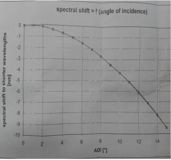
evaluate a transverse displacement of the beam, while changing the wave-length, equal to dx_dλ = 18 µm/nm, at a distance of 15 mm from the grating [6]. The corresponding angular dependence of the wavelength is dλ_dθ = 1.4 nm/mrad. Turning now to interference filters, the transmitted wavelength is given by [6]: λ = λ_⊥ � � � �1−sin2θ n2 ef f (2.1) where λ_⊥is the transmitted wavelength at normal incidence and nef f is

the eﬀective index of refraction for the filter (a tipical value is nef f = 2).

Taking θ = 6◦ and λ_⊥ = 853 nm, leads to |dλ

dθ| = 23 pm/mrad, which is

about 60 times smaller than for the Littrow configuration and demonstrates a substantial reduction of the wavelength sensitivity against mechanical in-stabilities. Finally, it is possible to demonstrate that the transverse dis-placement of the beam, consequently to the light tuning, is about two times smaller than for the previous configuration.

2.3 Our external cavity setup

2.3.1 Assembly of the mechanical components

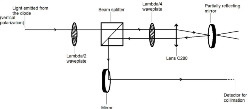
Figure2.1 shows a scheme of the external cavity optical configuration: the light emitted from the diode (DL) is collimated by a first lens (LC) with a short focal length of 3.1 mm. Then the collimated beam is focussed onto a partially reflecting mirror (OC) in a ”cat’s eye” configuration, formed by two lenses L1 and L2, of focal lengths 18.4 mm and 11.0 mm, respectively. The second lens provides a collimated output beam. The mirror is called here out-coupler and, thanks to the 30% reflective coating, provides the feedback into the diode. A piezo-electric transducer (PZT) attached to the mirror, allows to displace it in order to vary the length of the cavity. The optical

(27)

element called FI is the narrow-band interference filter mentioned above, that gives the frequency selectivity.

Figure 2.2: External cavity setup

Figure2.2 and 2.3 represent the various mechanical parts that constitute the external cavity setup. They are split up in three main assemblies labelled (1), (2) and (3). Part (1) is made up by two distinct sections, called (A) and (B) in the drawing. Figure2.3 gives an insight of part (1), and shows the various elements that compose it: our diode laser (T horlabs_{− L785P 090) is} set inside the copper disk (B4), directly in contact with a Peltier (B3) that ensures its termal stability. One first holder, made up by the two parts called

(28)

2.3. OUR EXTERNAL CAVITY SETUP 27

Figure 2.3: Insight of part 1

(B1) and (B2), keeps the diode and the Peltier together and a soft plastic ring (B5) ensures a good mechanical contact between the copper disk and (B2). Part (B) is locked between (A1) and (A2), thanks to the two screws (S5) and (S6) and part (1), as a whole, is fixed to part (2) by means of four screws placed at the edges of holder (A) and labelled (S1), (S2), (S3), (S4) in the figure. Finally, lens C330, that provides a first collimation for the light emitted from the diode, is placed inside the very right cylindrical edge of part (A2) and its position can be fixed by the three screws that we called (S10), (S11) and (S12).

Section (2) consists of three parts: (C) is a solid aluminum base, (D) forms the body of the external cavity, with two holes at its ends in which parts (1) and (3) will be positioned to form the external cavity and (E) is an aluminum holder for the interference filter. Part (E) can be rotated, so that the angle formed with the incident beam can be changed in order to select the right wavelength for the output beam. Its position can be fixed

(29)

through screw (S13).

Finally, part (3) contains the”cat’s eye” scheme. The first lens (C280) focusses the beam on the partially reflecting mirror and both are set into part (F ), while part (G) holds the second lens L2, that provides a collimated output beam. Part (3) can be fixed to part (2) through four screws, labelled (S14), (S15), (S16), and (S17). As far as the optical alignment of the system is concerned, the diode’s holder (B) was carefully positioned inside part (A) and we tried to make it as stable as possible, because even small perturbations in its position could cause a cutting in the shape of the laser beam, when the three main parts were put together.

2.3.2 The aligning procedure

A first collimation was provided by taking part (1) out from the cavity and choosing the right distance for lens (C330). Because the beam shape strongly depends on the position of section (B) inside holder (A), after a first rough choice for the position of (B) (good enough to ensure a non cut shape of the beam), we slightly tightened screws (S5), (S6) and then we did the last fine adjustment by little displacements of part (B) inside part (A), thanks to the three screws (S7), (S8) and (S9). The next step was to align the ”cat’s eye” scheme, with part (3) out from the cavity. We took as reference the beam just collimated by lens (C330) and, using the scheme shown in fig.2.4, we displaced lens (C280) in order to collimate the part of the beam reflected by the out-coupler. Eventually, the whole external cavity was built, and we optimized the collimation of the transmitted part, by means of lens (C220).

The beam axis out of the diode is defined by the metallic holder (B). We used screws (S7), (S8), (S9) and (S10), (S11), (S12) (that lock lens (C330)) for the vertical and horizontal alignment of the beam out of the diode holder (A). The first was performed measuring the heigth of the beam at different distances and we could obtain a vertical displacement of less than 1 mm over about 45 cm distance. If we consider that the cavity length is about 8 cm, it is possible to see a vertical misalignment lower than 0.2 mm between the two points at which light is emitted from the diode and reflected by the mirror. Assuming a good orientation of the mirror (i.e. such that the beam displacement after reflection is slightly affected by the mirror orientation), this implies a displacement lower than 0.4 mm at the diode position, after reflection, and this is sufficient in order to have a good overlap between the diode output and reflected beams for injecting the diode’s active area. For the horizontal alignment we used the filter holder (E) (without the filter in ) and we checked that the beam was symmetrically cut at both sides, when part (E) was rotated. As a consequence we could achieve a lower threshold current for the lasing effect to occur, from 31 mA without the cavity to 27 mA, when the external cavity was in.

(30)

2.3. OUR EXTERNAL CAVITY SETUP 29

Figure 2.4: Scheme of the design we used to align the ”cat’s eye”.

The interference filter is a bandpass filter, formed by a series of dielec-tric coatings on an optical substrate with anti-reflection coated back face. In order to reduce the production costs, optical filters are usually fabricated from larger wafers and then cut into pieces. The filter we choose belongs to a sample of 25 filters with diﬀerent bandpass wavelengths. They are 1 mm thick and have a surface area of 6× 6 mm2_{. We made use of a filter}

having 780.3 nm as nominal wavelength at normal incidence with respect to its surface. Figure2.5 shows the filter transmission curve given by the company datasheet, for a filter transmitting at about 780 nm. The curve refers to an incident beam forming an angle of zero degrees with respect to a unitary vector normal to the surface of the filter. The angle of maximum transmission depends on the wavelength and width of the transmission curve (specified at 0◦ incidence angle). The fullwidth at half maximum (FWHM) of the curve is about 0.12 nm and this is a good compromise in order to pro-vide suﬃcient discrimination for stable single mode lasing with satisfactory

(31)

output power. Indeed, higher finesse can be achieved at the cost of reduced transmission.

Figure 2.5: Typical transmission curve for a filter transmitting at 780 nm. Figure 2.6 describes the angular dependence of the spectral shift to shorter wavelengths for a typical interference filter in our sample. We will describe how interference filters act on wavelength stability in section 2.5.

(32)

2.4. THE FEEDBACK SYSTEM 31

Figure 2.6: Filter spectral shift with respect to the incident angle of the beam.

2.4 The feedback system: temperature and

wave-length stability controls

2.4.1 Sensitivity of the optical feedback for an

interference-filter-stabilized external-cavity diode laser

With optical feedback is meant the amount of light that can reach the active area of the diode after reflection on the partially reflecting mirror that forms one end of the external cavity. The optical feedback can be aﬀected by a misalignment of the external cavity with respect to the beam direction. If we consider a gaussian beam propagating through the cavity, whose direction is defined by the cartesian axis z, we can define as E0 and E2L the electric

fields at the position of the output facet of the diode after emission (z = 0) and after reflection on the out-coupler (z = 2L), respectively (where L is

(33)

the cavity length). The overlap integral of the emitted and reflected electric fields is a quantity that describes the feedback [6]

F = R−1��_�

� �

E∗₀(z = 0)E(z = 2L)dxdy��_�2 (2.2) where the reflectivity of the out-coupler R is a normalization factor. Therefore, the computation of the variation of F quantifies the mechanical and thermal sensitivity of the laser to a misalignment of the external cavity. The integral can be simplified if we evaluate it at the position of the out-coupler (z = L): F = R−1��_� � � E_i∗(z = L)Er(z = L)dxdy � � �2 (2.3)

where Ei is the electric field corresponding to the incident beam, while

Er is that of the reflected one. This simplification is possible because it

turns out that F is independent on the number of lenses inside the cavity [6]. Moreover, every displacement of optical elements can be transformed into two kinds of misalignment sources: tilt or axial displacement of the out-coupler. It turns out that, in the first case, for a small tilt angle [6]:

F = e−(απw0λ )2 (2.4)

while, if the reflective element is displaced along the optical axis: F =�1 +� δλ

πw₀2

�2�−1

(2.5) Here α and δ are respectively the angle formed by the incident and re-flected beam and the displacement of the mirror along the optical axis. w0 is

the waist of the incident beam at the out-coupler position, assuming normal incidence. If we now approximate the series expansion for the variation of F to the second order term:

dF = F��_� α=0+ α �_∂F ∂α ��_� α=0+ 1 2α 2�∂2F ∂α2��_α=0+ O(α 3₎ _(2.6)

and a similar expression for the feedback function with respect to the variable δ, it is possible to observe that the first order terms equal zero, while for the second order ones we have:

�_∂2_F ∂α2��_α=0=− 2π2w₀2 λ2 (2.7) �_∂2_F ∂δ2��_δ=0=− 2λ2 π2_w4 0 (2.8) These expressions show that w0 is the only parameter which determines

(34)

2.4. THE FEEDBACK SYSTEM 33 µm for the waist are typical for a system in which wavelength selection and optical feedback are independent tasks (like in our system in which the first function is fulfilled by an interfernce filter, while the second by a partially reflecting mirror) and this guarantee that only large deformations in both parameters α and δ (of the order of some mrad and tenths of mm, respectively) can decrease the factor F by 10%. On the other hand, a grating-tuned extended cavity laser (in which the previous two operations are carried out by the same diﬀraction grating), is characterized by much greater values for w0, typically of 1 mm magnitude. This makes the system

much more sensitive to external perturbations, and even a tilt of the grating of few hundreds µrad is suﬃcient to reduce F by a 10% factor [6].

The above analysis points out the advantages given by our ”cat’s eye” scheme, as far as the optical feedback is concerned. We will turn now to the electronic device we used for the temperature stability and wavelength control. The diode’s current supply was housed in a metallic box, assem-bled by Alessio Montori at LENS electronic whorkshop. This electronic system can be divided into three main parts: the diode’s current supply, the temperature controller and the driver for the piezo-electric transducer.

2.4.2 Description of the electronic system control

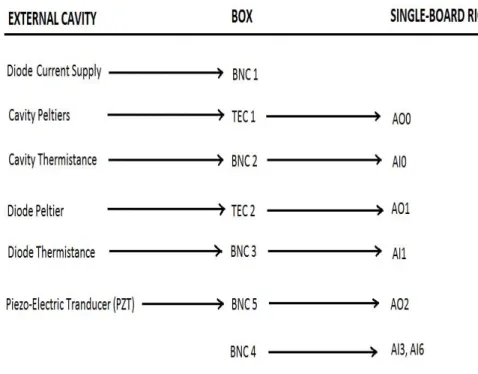
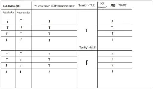
Figure2.7 is a scheme of the connections between the laser system (diode and external cavity), the metallic box containing the electronic components for the power supply and the electronic device that we used for the feedback system, while in fig.2.8 a front view of the metallic box, shows the three main parts mentioned above. On the left side we have the diode’s current supply the diode, and the output signal (BN C 1) is controlled by means of a potentiometer (P ot 1). Its value is monitored on the display and (Switch 1) commutes between current or voltage monitoring. The current is shown in mA units (and the corresponding voltage in mV ), with a resolution of 1 mA and a maximum value of about 200 mA. The middle part is devoted to the temperature feedback: (BN C 2) and (BN C 3) provide input voltage signals, representing the temperature of the external cavity and the diode, respectively. For each temperature stabilization unit, the temperature is converted into a voltage signal by means of a temperature-dependent resistor (thermistor) in a simple voltage divider formed by the thermistor and a stable 10kΩ resistor. The signal, once processed, is then converted into the output current feeding the Peltier cell. The connectors of output currents are labelled as (TEC1) and (TEC2) in figure2.8. The right part is for the piezo-electric tranducer (PZT) control. The voltage delivered to PZT through (BN C 5) is the sum of three contributions: an oﬀset voltage (controlled by means of (P ot 4)), a triangular, square or sinusoidal ramp, and a third one (correction signal) that can be added to the other two through (BN C 4) and whose function is to give the diﬀerence with respect to a reference

(35)

Figure 2.7: Scheme of the connections between the laser system components, the metallic box (whose front face is shown in fig.2.8) and the electronic de-vice we used for the feedback system (fig.2.9). The ”Diode Current Supply” is amplified inside the box without being processed by the sbRIO− 9636 (refer to fig.2.9), while the box input channel named BN C4 is needed for providing a signal to the sbRIO_{− 9636 device for the PZT control and thus} it is not connected to the laser system.

value; the electronic system for the PZT feedback will act in a way to make the error signal (i.e. the difference between the actual and reference signals before they are processed by a controller) equal to zero. While the offset is always present, the other two can be switched on or off using (Switch 2) for the ramp and (Switch 3) for the correction signal. Finally, (P ot 2) and (P ot 3) allow to change the ramp frequency and amplitude, respectively.

The electronic device that we used for the feedback was provided by National Instruments company and consists of two boards: a Single Board RIO (N I sbRIO_{−9636) and a National Instruments RIO Evaluation device.} The lower board is the sbRIO device, whose components are shown in figure 2.10.

The sbRIO is featured by a 512 MB nonvolatile memory and a 256 MB system memory (RAM). It can be supplied with a maximum DC voltage

(36)

Figure 2.8: Front view of the box containing the electronic circuit we used for the diode current supply, the temperature controller and the PZT driver.

of 30 V through the power connector (4), provides a number of digital and analog inputs/outputs and has an internal function generator, supplied with a battery that gives a maximum signal of 3.7 V. Component (8) is a ether-net port through whitch it is possible to interface the board to a Windows OS processor. The upper board is the NI RIO Evaluation device and it is connected to the sbRIO_{− 9636. The connectors J502 and J503 (numbers} (12) and (13) in figure 2.10), provide the pinout for all digital and analog inputs/outputs (I/O) on the Single-Board RIO and they are reproduced on

(37)

Figure 2.9: Picture of the electronic device for the feedback system: the lower board is the N I sbRIO_{− 9636, while the upper board is the NI RIO} Evaluation device and is connected to the first one.

the upper board. The device has 16 multiplexed,±10 V range, single-ended analog input channels, with 16-bit resolution and four analog output chan-nels with the same characteristics. Connector J503 provides analog inputs, outputs and grounds. On the other hand, connector J502 provides the 28 digital I/O. Some component oﬀered by the NI RIO Evaluation board are the six screw terminals for digital I/O [0:3] and two corresponding grounds, as well as six analog inputs ([0:5] plus one ground) and two analog outputs ([0:1] plus ground) screw terminals, as indicated in figure 2.9. Furthermore, the two potentiometers referred to as (P ot A) and (P ot B) in figure 2.9, allow a direct by hand access to the frequency and amplitude of the signal given by the embedded wave function generator. The two cursors (Cur A), (Cur B) allow to choose between three options for the frequency (0_{− 1 Hz;} 0− 10 Hz; 0 − 100 Hz) and shape (square, sinusoidal or triangular) of the

(38)

Figure 2.10: All possible components on the NI sbRIO Device.

signal. The last set of screw terminals (Sig Gen screw terminals) is for the output of the incorporated signal generator.

The two most important components of N IsbRIO− 9636 are the FPGA target (Spartan-6 LX25 type, distributed by Xilinx company) and the 400 MHz processor, labelled (15) and (17) in figure 2.10, respectively. A FPGA (Field Programmable Gate Array) is a chip with software programmable functionalities. It is made up by configurable logic blocks (CLB), that real-ize logic functions thanks to programmable interconnections between them, and input/output blocks (IOB) for data communication. With the

(39)

Lab-VIEW programmable FPGA target it is for example possible to realize logic functions for analog and digital I/O configurations, as well as realize op-erations concerning the LEDs and push buttons annexed to the NI RIO Evaluation device. On the other hand, the processor implements real-time operations and, establishing a communication channel with the FPGA, it is for instance possible to configure the LCD screen of the NI RIO Evalu-ation device for real-time monitoring applicEvalu-ations. In the following we will describe how, exploiting the FPGA, I have implemented the real-time tasks required for the diode’s temperature stability and piezo-electric transducer control.

2.4.3 The temperature control system: the Peltier

The physical components used for keeping the temperature stability of the external cavity and the diode are two Peltier elements with 6.0 A as maxi-mum supply current. One is set between elements (C) and (D) of part (2) in fig.2.2, while the other is located inside the holder (B) of part (1) (it is called (B3) in fig.2.3).

In order to present a short description of the Peltier effect we can consider an apparatus at constant uniform temperature, composed by two different metallic wires A and B that meet at two A/B junctions to form a closed circuit, and a battery that drives current around it. We can threat the system using a linear irreversible thermodynamic approximation, in terms of conjugate forces and fluxes and the related coefficients. According to the constraints imposed on the system, only heat and electrical charge currents will be present, and to first order approximation:

JQ= ∂JQ ∂FQ FQ+ ∂JQ ∂Fq Fq (2.9) Jq= ∂Jq ∂FQ FQ+ ∂Jq ∂Fq Fq (2.10)

Here JQ and Jq are the heat and charge current fluxes, while the

corre-sponding driving forces are:

FQ=−1 T dT dx (2.11) and Fq =− dφ dx (2.12)

where φ is the electrical potential and x measures the distance along the wires. In these relations the vector symbol for the physical quantities involved has been omitted, as we are considering all forces and fluxes to be parallel to each other. If we now define the direct and coupling coeﬃcients

(40)

2.4. THE FEEDBACK SYSTEM 39 LQQ ≡ _∂F∂JQ_Q, Lqq ≡ _∂F∂Jq_q and LQq≡ ∂J_∂FQ_q, LqQ ≡ _∂F∂J_Qq, and take into account

the boundary condition that the system is at constant temperature (which implies dT_dx = 0), we find a relation between the heat and charge currents, which is proportional to the ratio of the coupling (LQq) and direct (Lqq)

coeﬃcients:

JQ =

LQq

Lqq

Jq (2.13)

As these coefficients will have different values for the two metals A and B, therefore heat will accumulate and be emitted at one junction, while it will be absorbed at the other[8]. Thus, exploiting the Peltier effect, it is possible to build up a feedback system for temperature stability.

2.4.4 Temperature control system: the LabVIEW project

We briefly introduced the basic principle behind the implementation of logic functions on a FPGA chip. Here we are going to describe the details for the developement of the FPGA and Real-Time applications for our temperature stabilizing system. N IsbRIO_{− 9636 is a LabVIEW software programmable} device, and we used LabVIEW 2012 version to develop our program. Figure 2.11 shows a sequence of three sketches of the LabVIEW Project Explorer Window, in which diﬀerent targets are progressively expanded.

Let us look for the moment to the first sketch, placed to the left: we can observe a three level hierarchy, in which each level is indicated by a vertical line connecting two or more targets. The highest level refers to the Win-dows OS processor and to the Single-Board RIO device, which are connected through the ethernet port communication channel. The second level of the hierarchy corresponds to the target named ”Chassis(sbRIO_{−9636)”. It} rep-resents the Real-Time microprocessor (Component (17) in fig.2.10) and ev-ery real-time application will run under this target. The third and last level represents the FPGA and under the target ”F P GAT arget(RIO0, sbRIO₋ 9636)” it is possible to find all physical components belonging to the single-board RIO device and connected to the FPGA chip (component (15) in

fig.2.10). Finally, the targets we named as ”Real T ime M icroprocessor 20131125.vi” and ”Display temp setpoint plus buttons 20131125.vi”, placed under the

Real-Time and FPGA targets, respectively, are the two virtual instruments that we programmed on LabVIEW from the Windows OS interface. A virtual instruments represents an application capable to implement logic functionalities on the Single-Board RIO electronic device, as we could see later.

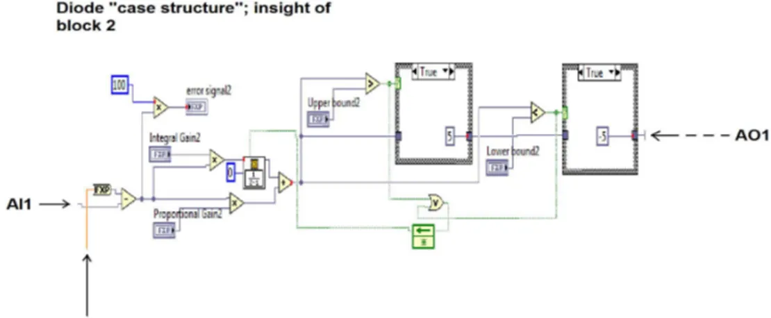
The purpose of our LabVIEW project is to develop a FPGA applica-tion for the configuraapplica-tion of analog inputs and outputs, in order to built a feedback system capable to stabilize the external cavity and diode temper-atures: we used two 10 kΩ thermistors that, depending on the cavity and

(41)

Figure 2.11: LabVIEW Project Explorer Window: three sketches of the same project are displayed, in which diﬀerent targets are progressively ex-panded.

diode temperatures, provide an input voltage signal to the Single-Board RIO. The device then acts to make this signal equal to a certain setpoint value, that fixes the final temperature for the system. The second task of the project is to implement a Real-Time application, to display the current setpoint values for both cavity and diode temperatures, as well as to

(42)

moni-2.4. THE FEEDBACK SYSTEM 41 tor their real time temperatures. Finally, for making this tasks independent from the Windows OS interface, we built a FPGA and a Real-Time stand-alone applications, that allow the FPGA and Real-Time virtual instruments to run automatically on the Single-Board RIO device.

T he F P GA V irtual Instrument

(43)

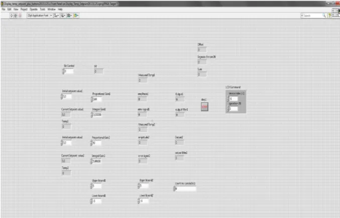
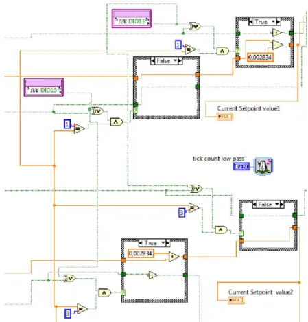
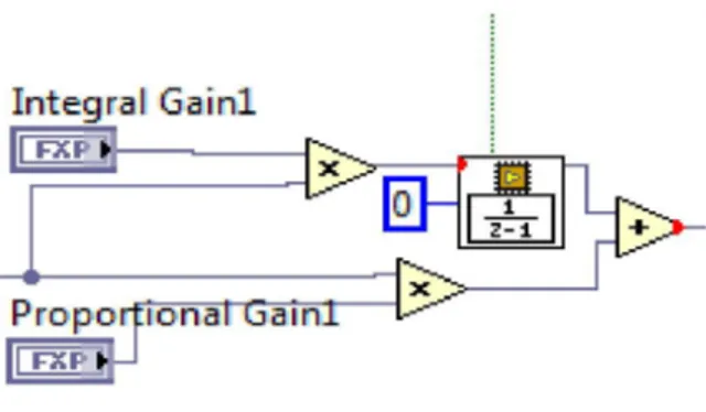
We will now examine the LabVIEW program concerning the FPGA Vir-tual Instrument (FPGA VI). Thanks to the Windows OS interface, a virVir-tual instrument can be viewed into two diﬀerent ways: through the VI Block Di-agram, that shows the LabVIEW functions that realize the logic blocks, or through the VI Front Panel, that provides a direct view of the values of the variables that belong to the VI Block Biagram.

Figure 2.13: FPGA VI Front Panel.