MKL - CT: Multiple kernel learning for censored targets

I..NIVmStTÀDEI.lACALABRIA

--..

".

()C'N1'UIDi~1A lJNlVE!ffiÀ.DEU.!\CALABf~

-==,.

DipartimentD di ELmRONICA, INFORMATICA E SISTEMISTICA

University of Calabria

Department of Electronics, Informatics and Systems

PhD course: Operations Research

Cyc1e XXI

Scientific sector: Operations Research (MA T/09)

MKL - CT: Multiple Kernel Learning for

Censored Targets

Candidate:

Vincenzo Lag~i

.

.

C\fÀrYWwt4'

~

Supe~or:

licJ57conforti

Coordinator of PhD course:

prof. Lucio Grandinetti

t)~

~~clAA-k~~,

Index

Introduction ... 1

1. Analysis of censored data... 3

1.1. Introduction... 3

1.2. Statistical approaches for the analysis of censored data... 5

1.3. Machine learning approaches for the analysis of censored data... 6

1.3.1. Data pre processing approaches ... 7

1.3.2. SVCR: Support Vector Regression for Censored Target ... 8

1.3.3. Survival Regression Tree and Survival Regression Forest... 11

1.4. Features selection and censored data. ... 11

2. Kernel Learning ... 13

2.1. Learning the kernel matrix ... 13

2.2. Kernel Learning with Semi Definite Programming. ... 14

2.3. Hyper Kernels. ... 16

2.4. Multiple Kernel Learning. ... 17

3. Multiple Kernel Learning for Censored Target. ... 21

3.1. Merging Support Vector Machine for Censored Target with Multiple Kernel Learning. ... 21

3.2. CT – MKL: optimization model. ... 23

3.3. CT – MKL: solving algorithm. ... 30

3.3.1. The wrapper algorithm ... 30

3.3.2. The chunking algorithm... 32

3.4. CT – MKL: implementation. ... 34

4. Experimentation... 39

4.1. Experiments Organization. ... 39

4.1.1. Experimentation protocol ... 41

4.1.2. Performance measure ... 43

4.2. Heterogeneous survival data: effect of the interaction among genetic and physiological factors for the ageing process. ... 45

4.2.1. Carolei dataset Description ... 45

4.3. CT – MKL on left, right, double and interval censored data... 50

4.3.1. Fried dataset Description ... 51

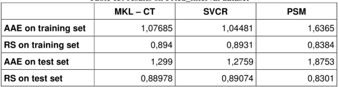
4.3.2. Experiments on Fried datasets ... 52

4.4. CT – MKL applied on real survival datasets. ... 57

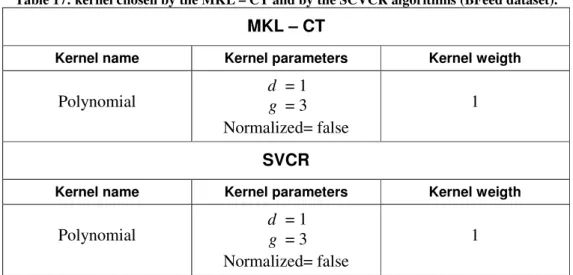
4.4.1. Experiments on Bfeed dataset... 57

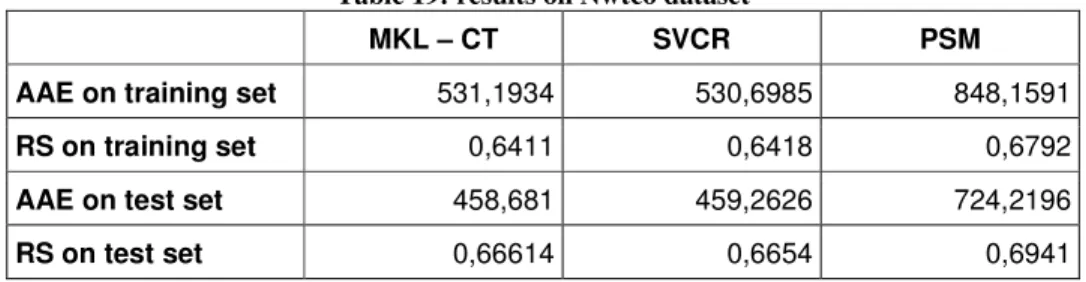
4.4.2. Experiments on Nwtco dataset... 59

4.4.3. Experiments on Pneumon dataset ... 60

4.4.4. Experiments on Std dataset... 62

4.5. Comparison of MKL – CT and SVCR algorithms in terms of time spent during the training phase. ... 63

4.6. Critical discussion of results. ... 64

Introduction

The analysis of censored data is a research stream of statistics science that attracted a great interest in the last decades. The term “censored data” indicates a uncertain measure known only through its upper and a lower bound. In particular, censored data are highly frequent in longitudinal studies, where the data to be collected consist in the times of occurrence of a particular event. Whether such event does not occur before the end of the study, one can only assert that the end of the study represents a lower bound for the actual time – to – event.

Recently, several Support Vector Machine (SVM) models were devised in order to deal with censored data. SVM consist in a class of Mathematical Programming models able to solve classification, regression and data description problems .In particular, the majority of SVM models can be stated and solved as Convex Quadratic Programming problems.

Beside SVM for censored data, in the last years other SVM models were introduced, able to automatically determine the best kernel function for the problem under study. Kernel functions can be thought as parameters of SVM models, that usually are chosen “a priori”. The performances of SVM models almost totally depend by the choice of the kernel function most suitable for the problem under analysis.

Summarizing, the current scientific literature offers both SVM models for dealing with censored data and SVM model able to automatically determine the best kernel to be used. An unique SVM model able to contemporary deal with censored data and to automatically select the best kernel is still missing.

Thus, the present thesis work consists in:

1. formulating the MKL – CT model, i.e. Multiple Kernel Learning for Censored Target. Such model unifies the characteristics of SVM model

for censored data and the features of MKL – SVM models for the automation of kernel selection procedure;

2. adapting MKL solving algorithms to the resolution of MKL – CT model; 3. modifying open source codes in order to solve the optimization problem

underlying the MKL – CT approach;

4. evaluating the effective validity of MKL – CT model through a wide experimentation carried out on simulated and “real world” data

It is worthwhile to underline the heavy role played by Operations Research and Optimization methods in the present thesis. In fact the MKL –CT model consists in a Quadratically Constrained Quadratic Programming model, that can be formulated as a Semi Infinite Linear Programming problem. Meanwhile, the solution of the final MKL – CT model can be obtained by using an “ad hoc” exact solving algorithm, belonging to the class of “exchange methods”.

In synthesis, even if this thesis is mainly oriented to the Machine Learning research field, the methods and models used during this work come from the latest developments of Optimization science.

Chapters are organized as following:

1. the first chapter introduces the main concepts related to censored data, and describes some of the methods used in order to analyze this type of data, including the SVM models for censored target;

2. the second chapter briefly outlines the SVM models able to automatic select the kernel function, with particular regard to MKL methods; 3. MKL – CT model and solving algorithm are deeply described in the

third chapter;

4. last chapter describes the experimentation performed and critically analyzes the obtained results.

1. Analysis of censored data

1.1. Introduction

Statistical modelling of time to event processes is a widely studied research field, with practical applications in many areas, including medicine, bioinformatics, actuarial sciences and reliability analysis.

For examples, numerous medical studies are carried out by registering the individual time – to – event of the subjects belonging to a selected population; the event under study can be the arising of specific symptoms, the development of an infection, or death. The aim of these studies generally is to analyze the effect of some factors (e.g. treatment, age) on the time to occurrence of the studied event.

If the event occurred in all subjects, many methods of regression analysis would be applicable. However, usually at the end of follow-up period some of the individuals have not experienced any event, and thus their actual time – to – event is censored, i.e. we only know that the event was not experienced until the limit of the follow up period. This type of censored data are defined survival data, and requires specific strategies in order to be analyzed; in particular, it is necessary to take in account the partial information provided by the censored times to event.

Survival data are also known as right censored data: the history of some subjects is not known after a certain time point, i.e., on the right side of an imaginary time line.

Other two types of censored data exist: when for some subjects it is only known that the event occurred before a certain time point, the data are defined left censored; when the censored times to event are known to lie between two time points, the data are said to be interval censored.

We can compactly model the three types of censored data using a mathematical formulation:

Let define a dataset D as a set of m tuples <xi,li,ui >, where each x represents i

the ith subject under study. The generic x_i can be indicated as subject, case or instance, and it is composed by n variables (called also attributes, features or

covariates), i.e. =< n> i j i i i i x x x x

x 1, 2,..., ,..., . The values l_i and u_i represent respectively the lower bound and the upper bound of the time to event y_i of the generic ith subject.

Given this formulation, we can easily represent left, right and interval censored cases, as well as the cases with a known time to event:

• left censored cases are characterized by l_i=−∞;

• right censored cases by ui=+∞;

• interval censored are represented allowing ui > ; li

• cases with known time to event have u_i = . l_i

Other formalization could be adopted in order to represented censored data; we chose the above given formulation because it is highly intuitive and it will allow an easier explication of some concepts in the following chapters.

Moreover, it should be noted that the adopted formalization is not able to represent some more complex information, such as time varying variables, presence of multiple events, censored covariates. However, these kind of data (and the respective methods of analysis) will be not considered during the present thesis.

Instead, the main aim of the algorithms and methods presented in the rest of this work can be described with the following proposition:

Proposition 1: Given a dataset D, find a function f :Rn →R able to represent the relationship between the set of variable x and the time to event y , i.e.

) (x f

y= . The time to event y is known only through its lower and upper bound, respectively l and u .

1.2. Statistical approaches for the analysis of censored

data

Over the last decades, censored data analysis received increasing interest by the statistical community. Several parametric and semi parametric algorithms were developed in order to modelling time to event on a set of covariate, even in presence of censored data: one of the first and most notable technique is the semi parametric Cox regression model [1]. More recently, other methodologies were developed, including parametric survival models [2], accelerated failure time models [3], spline based extensions [4], fractional polynomials [5] and Bayesian methods [6].

Among the afore cited techniques, Cox regression and parametric survival models deserve a more detailed explication, for their wide use in the analysis of censored data.

Cox regression models were originally developed for survival data, and in their original form they can deal only with right censored cases. Cox regression lies on the definition of the survival function S

( )

t =Pr(T >t), that is the probability of surviving after the time t. The hazard function, defined as h(t)=−S'

( ) ( )

t S t , express the risk of experiencing the event at time t.

In his famous work [1], Sir Cox proposed to model the hazard function with the following formula: x bT e t h x t h(, )= 0()⋅

where h0(t) is a baseline hazard function, common to all the subjects, and the

terms bTx

e takes in account the influences of a set of covariates x , representing the particular status of each subject.

The points of strength of Cox models are:

1. the estimation procedure of parameters vector b is based on the maximization of the log likelihood and is able to exploit the information carried out by the censored cases;

2. the baseline hazard function must not be estimated in order to calculate the value of the parameters vector b.

On the other hand, Cox models assume that the hazard ratio between two subject will be constant over the time, i.e. the ratio between the hazards of subject A and subject b will remain the same independently by the time. Of course this assumption represent a limitation for the Cox models.

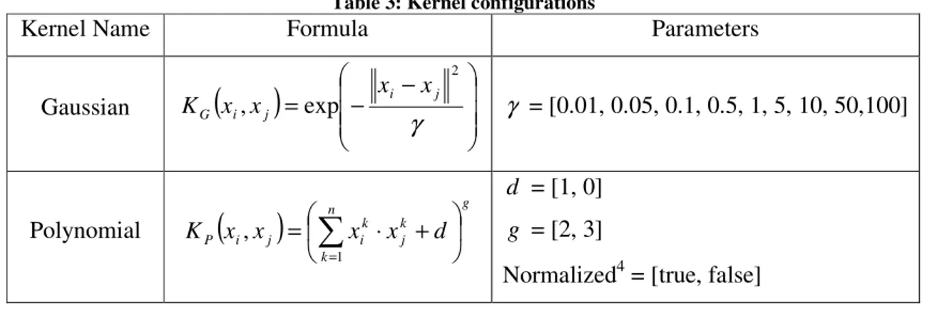
Parametric survival models assume that the survival function of a population can be modelled with a given parametric distribution. Some of the most used distributions are shown in Table 1. Survival functions are unconditional, in the sense that they do not take in account the vector of covariates characterizing the different subjects. Then, survival functions must be turned in conditional models, by replacing one of the free parameters with a (suitably transformed) linear predictor. The linear predictor is simply the inner product of a parameters vector b and the vector x of the covariates under study.

Table 1: Survival distributions for parametric survival models. The cumulative normal distribution φ(z) is defined as

∫

∞ − Ν = z d z γ γ φ( ) ( ;0,1) . Distribution S(t) Weibull exp(−λ⋅tγ) Exponential exp(−λ⋅t) Log – Normal 1−φ(λ⋅ln(t)) Log – Logistic 1 ) 1 ( + ⋅ γ − λ t

1.3. Machine learning approaches for the analysis of

censored data

Various algorithm aimed to deal directly with censored data were developed in the context of the machine learning community.

Generally speaking, Machine Learning algorithms for survival analysis mainly consist in previously existent algorithms specifically modified or re – formulated in order to take in account censored samples. Among the various works present in

for censored data [7], Artificial Neural Networks [8], Survival Ensemble and Survival Random Forest [9], Supervised PCA [10] and SVM like algorithms [11, 12, 13]. Moreover, there exist also some examples of statistical techniques hybridized with machine learning elements, such as Kernel Cox regression model [12] and Kernel accelerated time survival analysis [14].

Even if not limited to the above list, machine learning techniques able to deal with censored data remains relatively few, and moreover free software implementations are very rare. Exceptions are Survival Random Forest and Hierachichal Mixture of Experts (HME) models, both available for the R software in their respective packages “randomSurvivalForest”1 and “hme”2.

The following paragraphs will deeper explain some of the techniques afore mentioned, with particular emphasis on SVCR and Random Survival Forest (RSF). SVCR has been successively used during the experimental tests.

1.3.1. Data pre processing approaches

Several strategies based on data manipulation have been proposed in order to let machine learning algorithms deal with survival/censored datasets. This approaches are mainly concerning on right censored data.

The simplest method considers survival for a fixed time period, and consequently gives a binary classification problem [15]. Censored observations are removed and biases are introduced. It is clear that this approach is rather basic and does not really deal with the problem of censoring.

A second approach is based on multiple replications of each subject [15]. According to this method, each instance x_i is replicated several times, with two more attributes added to each replica:

1. an increasing “time stamp” n+1 i

x ;

2. a class attribute y_class indicating whether the event occurred or not at the

time n+1 i

x

The converted dataset can be processed using the standard algorithm for classification problems. This approach has been widely used in the field of neural network, and several publications testify its effectiveness [16 – 19]. Nevertheless, the replication of the original instances can produce scalability problems, due to the dimensions reached by the converted dataset.

The third approach consists in the imputation of censored outcome using the information carried by the uncensored cases. This method require a hierarchical structure of regression models: one or more models are firstly trained on the basis of the uncensored instances in order to estimate the times to event for the censored cases. Then, the final model is trained utilizing all the cases, using the estimated times to event for the censored cases [20].

1.3.2. SVCR: Support Vector Regression for Censored Target

SVCR represents one of the last attempts of adapting the well known SVM models to the analysis of censored target. Numerous tutorial regarding the standard SVM models are available for the interested readers [21].

Recalling the concepts expressed by Proposition 1, the main idea at the basis of the SVCR models is that the function f(x_i) should respect the following condition:

i i i f x u

l ≤ ( )≤ i₌₁Km

that is, the estimations of times to event y provided by the function f should respect the upper and lower bounds u and l .

Let suppose that the function f consist of a simple linear combination of

variables x , i.e. f(x_i)=wT ⋅x_i+b. Then, condition (1) could be expressed with the following constraints:

0 ≤ − + ⋅ i i T u b x w ∀i∈U 0 ≤ − ⋅ −w x b l T L i∈ ∀ (1) (2) (3)

where U is defined as U =

{

i|u_i <+∞

}

and L=

{

i|l_i >−∞

}

.

Usually real world data do not follow a strict liner trend, as required by constraints (2) and (3); then some slack variables should be added in order to make such constrains generally feasible:

∗ ≤ − + ⋅ _{i i i} T u b x w ζ ∀i∈U i i T i w x b l − ⋅ − ≤ζ ∀i∈L 0 ≥ i ζ , ∗ ≥0 i ζ i∀

Following the regularization theory, that is one of the main pillar of SVM methods, the weights w can be uniquely determined by imposing the minimization of w norm [22]. Then, the final primal optimization model is the following:       + +

∑

∗

∑

∗ i i i i b w C w ζ ζ ζ ζ 2 , , , 2 1 min ∗ ≤ − + ⋅ i i i T _{x b u} w ζ ∀i∈U i i T i w x b l − ⋅ − ≤ζ ∀i∈L 0 ≥ i ζ , ∗ ≥0 i ζ i∀

where C is a user defined parameter.

Model (7) – (8) is the primal form of the SVCR optimization problem. Assigning dual variables α∗ and

α

to constraints (8) and (9), the following dual problem can be easily obtained:

(

₋ ∗

)(

₋ ∗

)

(

)

_{−Λ +Ψ} ∗

∑∑

∗ α α α α α α α α T T i j j i j j i i K x ,x 2 1 min , 0 = − α∗ α T U T L e e 0 , 0≤_{α α}∗ ≤ _i∀ (5) (4) (6) (10) (8) (7) (12) (13) (6) (9) (11) (6) (10)

In constrain (12), vectors e_L and e are defined as: _U

[ ]

   =−∞ = otherwise l if e_{L i} i 1 0

[ ]

   =+∞ = otherwise u if e_{U i} i 1 0

Similarly, vectors Λ and Ψ are defined ad:

   =−∞ = Λ otherwise l l if i i i 0    =+∞ = Ψ otherwise u u if i i i 0

The kernel function K

(

x_i,x_j

)

replaced the scalar product in the objective function (11) in order to allow a non linear decision function.

Model (11) – (13) formally is equivalent to the standard dual Support Vector Regression model [22]. Numerous fast and scalable algorithm have been developed for the solution of this type of quadratic program, as for example the SMO algorithm [23]. The size of the problem is equal to 2⋅n, while the. complexity is in the order of O

( )

n2 .

A few lines should be spend in order to define the elegant properties of this model. Firstly, SVCR is totally non parametric, in the sense that no assumption are made regarding the distribution of the data or about the shape of the survival/hazard function. The absence of assumptions regarding data distribution is a great advantage of SVCR in respect of classical statistical models, as for example Cox regression.

Moreover, SVCR is able to provide estimates of the time to event y for left, right and interval censored data, while other machine learning or statistical methods are ale to deal only with right censored cases.

Finally, SVCR optimization problem can be faced with all the efficient algorithms specifically developed and implemented for solving the standard SVM optimization problem; pre – existent codes for SVM solution can be easily adapted for SVCR particularities.

1.3.3. Survival Regression Tree and Survival Regression Forest.

Survival regression tree have been firstly introduced by M.R. Segal [7] for the analysis of right censored data. The main idea consists in recursively subdividing the dataset D until it is not possible to recognize two groups with significantly different survival functions within the final subsamples.

The algorithm examines singularly each variable, and test whether it is possible to subdivide the sample in two or more subgroups with different survival functions; once tested every variable, the sample is subdivided following the variable that allows the creation of the subsamples most dissimilar. The iteration is repeated on each subsample until any subdivision is possible. A statistical test is usually used in order to assess the diversity of two survival functions.

An evolution of such algorithm is represented by the Random Survival Forest (RSF) algorithm [24]. RSF algorithm merge the Breiman’s Random Forest [25] with the survival regression trees, trying to exploiting the advantages of both methods. Random Forest algorithms construct several decision trees, randomly or pseudo randomly choosing the nodes of each tree. When a new instance is presented to the Random Forest to be evaluated, each tree give an evaluation, and then a voting procedure is used over all the predictions. RSF use this same schema, adding the subdivision rule based on a statistical test for comparing two or more survival functions.

A freeware implementation of RSF algorithm is freely available as a package of the R software

1.4. Features selection and censored data.

methods specifically devised for selecting the most relevant features for classification and regression problems.

However, much less work has been done regarding features selection in presence of censored outcomes. In particular, only few algorithms have been specifically devised in order to directly deal with censored data.

Univariate and wrapper features selection methods can be used also with censored data, choosing the appropriate statistical test (e.g. log rank test) for the univariate selection and a suitable performance function for the wrapper algorithms (for example, the C index [26]).

Beyond univariate and wrapper methods, other features selection algorithms for censored dataset have been developed within the bioinformatics area.

In bioinformatics studies, datasets are usually composed by thousands of variables and relatively few (hundreds) cases. Then an effective selection of the most relevant variables is mandatory. An extensive review of such methods has been written by Bøvelstad et al [27].

2. Kernel Learning

2.1. Learning the kernel matrix

Kernel based methods gained increasing popularity over the last years. One of the main reasons of kernel methods success relies on the so – called “kernel trick”, i.e., the possibility of replacing simple dot products with a more complex, and usually more effective, kernel function.

Kernel functions are not a trick merely useful in order to catch non linear trends present inside data; using the kernel functions, it is possible to embed domain specific knowledge inside general purpose data analysis algorithm, specifying a “similarity measure” able to incorporate the specificity of the problem under analysis. Then, several kernel functions have been devised and successfully experimented in various application field, from genetic sequences analysis to speech recognition [28] [29].

However, kernel methods presents also some drawbacks. The principal issues consists in the need of choosing a suitable kernel function: the performance of any kernel based algorithm is strictly depending by the choice of the similarity function. Generally, machine learning algorithms present several parameters to be set by the user; a reasonable choice of such parameters allow the algorithm to best fit the data. On the other side, unwary parameters setting techniques can easily lead to data over fitting, so time expensive performance estimation techniques, as for example cross validation, must be used in order to provide unbiased estimates of the performance for each tested parameters configuration.

From this point of view, the selection of the most suitable kernel can be seen as part of the parameters setting procedure. Moreover, it should be noted that kernels usually have some own parameters to be set, adding a further level to the parameters setting problem. When the choice of the kernel is enumeratively performed, the kernel selection process can be thought as a discrete optimization problem: given a dataset D, a kernel based algorithm A, a set K of kernel functions, K =

{

K1,K2,K,K_K

}

, and a performance estimation procedure P, find

Recently, new methods have been proposed in order to partially overcome the kernel selection problem, when SVM models are used. Such methods can be comprehensively named as Kernel Learning algorithms, since they attempt to contemporarily learn SVM model variables and the most suitable kernel directly from data.

The advantages of such approach are evident: a direct estimation of the kernel metric allows to avoid time consuming kernel selection procedures. Moreover, from a theoretical point of view, kernel estimation should provide more suitable similarity function compared to the usual selection procedure based on the experimentation of several “a priori” chosen kernels.

On the other hand, Kernel Learning approaches present some disadvantages: the computational effort required in order to train a Kernel Learning based SVM is usually far away more consistent than the effort required by the training of a standard SVM model. Moreover, known Kernel Learning algorithms can not learn new similarity functions without the specification of the typology of kernel to be learnt or without an initial set of kernels to be together combined.

Kernel Learning approaches first appeared in 2004, with Lanckriet et al. paper [30], proposing a Kernel Learning approach based on Semi Definite Programming (SDP) [31]. Other approaches have been successively developed by Ong et al. [32] and by Sonnenburg et al. [33], respectively proposing Hyper Kernels and Multiple Kernel Learning (MKL) methods.

The following paragraphs will introduce the main ideas of the afore mentioned approaches, with their respective points of strength and disadvantages. MKL methodology will be widely explained and discussed in the chapter 3, since the main results of the present thesis work are based on MKL techniques.

2.2. Kernel Learning with Semi Definite Programming.

Lanckriet et al. proposed to estimate the kernel matrix as the linear combination of a set K of known kernel functions:

∑

= ⋅ = K k k k K K 1 β (14)

Starting from this simple idea, the authors demonstrated that Kernel Learning can be formulated as an SDP problem. Let recall the standard dual SVM model for classification tasks:

( )

: 0, 0

2

max ⋅_αTe−_αTG K _α C≥_α≥ _αTy=

α

where y represents the labels vector (yi =±1) and G(K) is defined as:

( )

[

G K

]

_ij = y_i⋅y_j⋅K(x_i,x_j)

Merging expression (14) and (15), it is possible to demonstrate that the final model can assume the form:

t r T t ⋅α−µ ⋅ α 2 max ,

( )

K k K G r t T _k k K , 1 1 = ⋅ ≥ α α 0 , 0 ≥ ≥ = α αTy C

that is a SDP model, where r_k =trace

( )

K_k and under the adjunctive constraint 0

≥

µ .

The great advantage of SDP model (16) – (18) is its convexity, ensuring that no local minima might be found. On the other hand, model (16) – (18) has a computational complexity in the order of

(

3

)

m K

O ⋅ , far away superior to the

usual O

( )

m2 complexity of standard SVM models.

Moreover, the authors experimented their model only within the limits of a transduction setting, and they did not provide a version of the model for the induction tasks.

(15)

(16)

(17)

2.3. Hyper Kernels.

The approach developed by Ong et al. is conceptually different from the work of Lanckriet et al., but the final model is again formulated as an SDP problem.

The main idea of the Hyper Kernel approach consists in minimizing the regularized risk with respect to both function f and the kernel function K .

Let recall the standard primal SVM model for classification task:

∑

= + m i i b w w C 1 2 , ₂ 1 min ζ m i b x w y_i⋅( T _{i + )≥1−ζi, ζ ≥0i, =1}K

where yi=±1 represents the label assigned to each case. The term w 2 1

is the

regularization term, ensuring the required properties of robustness and uniqueness

of the function f . The term

∑

= m i i C 1

ζ represents the loss function, that is, the admitted inaccuracy of the function f with respect to the training data.

Recognizing that the function f could assume multiple form, and that the loss function could be generally represented as a function l

(

x_i,y_i,f

)

, then the model (19) – (20) can be rewritten as:

(

)

∑

= ⋅ + m i i i f f C l x y f 1 2 , , 2 1 min

The idea of the Hyper Kernel approach simply consists in adding an adjunctive terms K to model (21), in order to minimize also the regularized risk related to

the choice of the kernel function:

(

)

2 1 1 2 , ₂ , , 1 min f C l x y f C K m i i i K f + ⋅

∑

+ ⋅ = (19) (20) (21) (22)

where C1 is an user defined parameters. The introduction of the term K

require the definition of a Hyper Kernel function, able to provide the dot product of two kernel functions as calculated in some Reproducing Hilbert Space.

Starting from model (22), it is possible to demonstrate that the final model assumes the shape of a SDP model. The final model is convex, and ensure the existence of a unique global minima.

However, also Hyper Kernel approach presents multiple disadvantages. In particular, the SDP models require the definition of more than 2

m variables, where

m is the number of training instance, leading to scalability problems. Moreover, the Hyper Kernel approach does not eliminate the problem of choosing a suitabl kernl problem, because such approach requires an “a priori” definition of a Hyper Kernel function, so the problem of choosing a suitable kernel is only moved to a higher level. Lastly, Ong et al. justified their work as a solution able to effectively deal with the presence of attributes with different variances/scale factors; however, such types of issues can be more easily resolved by using a pre processing step, as normalization or standardization of the variables. So, the practical usefulness of such approach could be questionable.

2.4. Multiple Kernel Learning.

The MKL approach start from the same idea of Kernel Learning with SDP: the kernel function is defined as the linear combination of a set of already known kernel functions, as modelled in the expression (14).

The difference between the two methods consists in the final optimization model used in order to resolve the SVM model once the linear combination of kernel is embedded inside the standard Support Vector Machine model.

In order to develop their model, Sonnenburg et al. started from the classical primal SVM model for classification problem, modifying the regularization term:

∑

∑

= = +         m i i K k k C w 1 2 1 2 1 min ξ (23)

n i b x w y K k i T k i 1 1K 1 = − ≥         +

∑

= ξ 0 ≥ ξ

The dual version of model (23) – (26) can be written as:

γ min K k x x K y y n i i n i n j j i k j i j i ( , ) 1K 2 1 1 1 1 = ≤ −

∑

∑∑

= = = γ α α α C yTα =0, 0≤α≤

It should be noted that a different kernel K has been defined for each _k w . _k Moreover, the left side of inequality (28) is the objective function of a standard SVM model; let assume

( )

∑∑

∑

= = = − = n i i n i n j j i k j i j i k yy K x x S 1 1 1 ) , ( 2 1 α α α α .

Interestingly, the dual version of model (26) – (28) can be written as the following: θ max

( )

|0 , 0 1 = ≤ ≤ ℜ ∈ ∀ ≥ ⋅

∑

= α α α θ α β n T K k k k S C y k k K k k = ≥ ∀

∑

= 0 , 1 1 β β

The model (30) – (32) deserves some adjunctive explications. Firstly, it should be noted that the model is linear with respect to θ and β; however, line (31) potentially defines infinite linear constraints, because it should be considered one

(24) (25) (26) (27) (28) (30) (31) (32) (29)

constraint for each admissible values of the vector _∈ℜn

α . So expressions (30) – (32) define a Semi Infinite Linear Program (SILP) [34] model.

Compared with SDP and Hyper Kernel methods, MKL presents several advantages. In particular, it should be noted that:

1. MKL allows for effective Kernel selection. MKL provides vector β at the end of the optimization process; the β coefficients can be interpreted as the relative importance of each kernel, i.e., kernel functions more influencing on the solution will have a greater weight. Then, MKL can be used as a tool for kernel selection, in the sense that irrelevant kernel will not enter in the solution because their respective β_k will be zero. This particularity is considerably useful during the practical usage of SVM methods. In fact, MKL allows to contemporary experiment several kernels, avoiding the need of singularly test each kernel function. In some sense, with MKL it is possible to pass from an enumerative, discrete search of the best kernel to a search in the continuous space of kernels combination.

2. MKL allows the merge of heterogeneous data. Let re – write the line (24) in the following way:

n i b x w y K k i k T k i ( ) 1 1K 1 = − ≥         + Φ

∑

= ξ

where Φ is a projection among the attributes of _k x_i, i.e. each Φ _k selected a different subset of variables. Model (30) – (32) is not modified by this change; however, with such modification each kernel is applied only to a subset of dataset attributes. Let suppose that data under study are composed both by clinical and genetic information; in such a case, projections Φ will subdivide the two typologies of data, allowing the _k contemporary experimentation of different kernels on clinical and genetic data. Under this respect, the coefficient β indicate the relative importance of each attributes subset, allowing an interpretation of the

respective attributes subset, and conversely a very small β value will indicate a irrelevant set of attributes.

3. Effective and scalable algorithm have been developed for the solution of model (30) – (32), and efficient implementation of such methods are public available. This point will be largely discussed in the next chapter.

For sake of clarity, it should be underlined that properties at point 1) and 2) are common to MKL and SDP approach, while the Hyper Kernel approach seems not able to perform kernel selection or features relevance analysis.

3. Multiple Kernel Learning for Censored Target.

3.1. Merging Support Vector Machine for Censored Target

with Multiple Kernel Learning.

In previous chapters two important research areas were introduced and discussed: the analysis of censored data and the Multiple Kernel Learning techniques.

Both research areas address relevant problems: the analysis of censored data allows a complete utilization of the information/knowledge hidden in censored/truncated dataset; on the other hand, MKL methods greatly improve the already effective and efficient kernel based methods.

In particular, it is worth while to remind that MKL can be used both for automatic kernel selection and for the effective analysis of heterogeneous data (see chapter 2).

However, the current literature does not report any attempt to merge this two distinct fields: that is, there is not any machine learning technique able to analyze censored data exploiting the advantages of MKL techniques. Let call this hypothetic technique “CT – MKL”.

It cold be stated that maybe there is not the need of creating a technique able to merge MKL and censored data analysis. Instead, it is easy to demonstrate that several “real world” problems could be faced in a much more effective way by an hypothetic CT – MKL technique.

Let have a practical example in order to better explain the need of creating a bridge between censored data analysis and MKL.

In the last decades, genetics studies focused on discovering the causes of complex phenotypes: questions like “which are the genetics characteristics responsible of mental skills?” or “which is the role of genetic predisposition in the process of ageing?” have been largely debated among biology and bioinformatics community.

However, the genetic component influencing the development of complex phenotypes rarely is preponderant with respect to other factors, like for example the characteristics of the ambient where the subjects under study grew and live, the alimentary diet, education, and so on.

Usually, in order to have a global picture of the causes of a particular complex phenotype, heterogeneous data must be collected, registering both genetics and not genetics information. Then all the information should be together examined, in order to take in account the possible interactions among the various factors.

Moreover, some complex phenotypes can be represented as an event occurring during the time; the most clear example is life duration, also known as life expectation. Usually, studies carried out on expectation of life must face the problem of censored data, due to subjects early dropping out from the study.

Synthesizing, the study of interactions among genetics characteristics, not genetics factors and life expectations is a typical problem that could gain great advantages from a technique able to merge MKL and censored data analysis; in fact, the presence of various factors suggest the use of a technique able to deal with heterogeneous data, like MKL; on the other side, the occurrence of censored cases need the application of a technique able to deal with censored data.

Moreover, it should be reminded that MKL can be used as an automatic kernel selection procedure; then, each kernel based methods able to deal with censored data could obtain advantages by MKL techniques, at least in terms of time savings during the parameters optimization phase.

Once explained that it is necessary to create a CT – MKL technique, it must be decided how to realize such ideas. A very straightforward solution would be merging MKL techniques with one of the SVM models able to deal with censored data. As pointed out in the brief literature review given in Chapter 1, SVCR presents several advantages with respect to other SVM implementation for censored data, i.e. the possibility of deal with right, left and interval censored data, and the possibility of using highly efficient optimization algorithms.

Then, the most natural choice in order to create a CT – MKL algorithm seems to be the fusion between the SVCR model and MKL techniques.

The objective is obtaining a model with the advantages of both SVCR and MKL techniques, in particular:

1. the ability of dealing with right, left and interval censored data; 2. the possibility of effectively treating heterogeneous data; 3. the ability of performing automatic kernels selection;

4. fast and effective algorithm for the solution of the underlying optimization problem.

The following paragraphs will introduce the CT – MKL model in detail, together with the optimization algorithm and the implementation strategies adopted in order to realize the software code.

3.2. CT – MKL: optimization model.

In this paragraph we will derive the optimization model of CT – MKL technique. Let recall the primal SVCR model as given in paragraph 1.3.2:

      + +

∑

∑

∈ ∈ ∗ ∗ U i i L i i b w C w ζ ζ ζ ζ 2 , , , 2 1 min ∗ ≤ − + ⋅ i i i T u b x w ζ ∀i∈U i i T i w x b l − ⋅ − ≤ζ ∀i∈L L i i≥ 0∀ ∈ ζ , _i∗≥ ∀i∈U 0 ζ

With respect to model (34) – (37), we introduce a slightly modification, by setting up a further user defined parameter ε ; the modified model have the following form:

(35) (34)

(37) (36)

      + +

∑

∑

∈ ∈ ∗ ∗ U i i L i i b w C w ζ ζ ζ ζ 2 , , , 2 1 min

(

₊

)

_≤ ∗ − + ⋅ i i i T u b x w ε ζ ∀i∈U

(

)

i i T i w x b l −ε − ⋅ − ≤ζ ∀i∈L L i i≥ 0∀ ∈ ζ , _ζi∗≥₀∀i∈U

ε introduction produces two different effects. Firstly, model (38) – (41) is more easily resolvable, because ε relaxes the constraints (39) and (40).

Secondly, the introduction of ε allows the use of the so – called “ε insensitive loss function”, i.e. the estimations f(x) of times to event y are required to be comprised in the interval

[

l−ε;u+ε

]

. In other world, high values of ε will provide a function f(x) able to better reproduce the general trends of the data, while low ε values will generate a regression function more faithful to the training data.

Once redefined the primal model of SVCR, let merge the MKL model (23) – (26) with model (38) – (41):       + +        

∑

∑

∑

∈ ∈ ∗ = ∗ U i i L i i K k k b w C w ζ ζ ζ ζ 2 1 , , , 2 1 min

( )

(

_⋅Φ

)

_{+ −}

(

₊

)

_≤ ∗

∑

i i k i k T k x b u w ε ζ ∀i∈U

(

)

(

( )

)

i k i k T k i w x b l −ε −

∑

⋅Φ − ≤ζ ∀i∈L L i i≥ 0∀ ∈ ζ , _i∗≥ ∀i∈U 0 ζ

Note that w_k can be written as w_k =β_k⋅w'_k , under the further constraints

∑

= = K k k 1 1

β and β_k ≥ 0∀k . For sake of simplicity, thereafter x_ik will be used instead of Φ_k

( )

x_i ; moreover, index k will range from 1 to K , unless otherwise

(39) (38) (41) (40) (43) (42) (44) (45)

specified. In their paper [35], Bach et al. derived a dual version of problem (42) – (45) by treating the primal model as a Second Order Cone Programming (SOCP) optimization problem.

Let define the following cone constraint:Cone_k =

{

(w_k,t_k)∈ℜK+1| w_k ≤t_k

}

; problem (42) – (45) can be now written as:

      + +

∑

∑

∈ ∈ ∗ ∗ U i i L i i b w C ζ ζ δ ζ ζ 2 , , , 2 1 min

(

_⋅

)

_{+ −}

(

₊

)

_≤ ∗

∑

i i k ik T k x b u w ε ζ ∀i∈U

(

)

(

)

i k ik T k i w x b l −ε −

∑

⋅ − ≤ζ ∀i∈L

∑

≤ k k t δ

(

w_k,t_k

)

∈Cone_k ∀k 0 ≥ i ζ , ∗ ≥0 i ζ i∀ Note that

∑

≤

∑

≤δ k k k k t

w , then model (46) – (51) and model (42) – (45) are

equivalent. Taking in account that constraint (50) is self dual, the Lagrangian function of problem (46) – (51) can be written as:

(

)

(

)

+      − + − + ⋅ ⋅ +       + + =

∑

∑

∑

∑

∈ ∗ ∗ ∈ ∈ ∗ U i i i k ik T k i U i i L i i w x b u C L δ2 ζ ζ α ε ζ 2 1

(

)

(

)

− − +      − − ⋅ − − ⋅ +

∑

∑

∑

∑

∈ ∗ ∗ ∈ ∈ iU i i L i i i L i i k ik T k i w x b B B l ε ζ ζ ζ α

(

)

∑

∑

− ⋅ + ⋅      − + k k k k T k k k w t t δ λ µ γ L i i≥ 0∀ ∈ α , _i∗≥ ∀i∈U 0 α 0 ≥ γ

(

λk,µk

)

∈Conek (47) (46) (48) (49) (50) (51) (52) (54) (53) (55)

Let derive the Lagrangian function (52) with respect to variables δ , t , b , ζ , ∗ ζ , w : γ δ γ δ δ = − = ⇒ = ∂ ∂ 0 L k t L k k k ∀ = ⇒ = − = ∂ ∂ µ γ µ γ 0

∑

∑

∈ ∈ ∗_{− =} = ∂ ∂ U i i L i i b L 0 α α L i B C B C L i i i i i ∈ ∀ − = ⇒ = − − = ∂ ∂ α α ζ 0 U i B C B C L i i i i i ∈ ∀ − = ⇒ = − − = ∂ ∂ ∗ ∗ ∗ ∗ ∗ α α ζ 0

(

)

x k w L k m i ik i i − − = ∀ = ∂ ∂

_∑

= ∗ 0 1 λ α α

Replacing expressions (56) – (61) in model (46) – (51), we obtain:

(

)

∑

(

)

∑

∈ ∈ ∗ − ⋅ + + ⋅ − − L i i i U i i i u ε α l ε α γ2 2 1 min k k k ≤µ ∀ λ k k =γ ∀ µ

(

)

x k m i ik i i k =

∑

− ⋅ ∀ = ∗ 1 α α λ

∑

∑

∈ ∈ ∗_{− =} U i i L i i α 0 α m i C i i, 1K 0≤_{α α}∗≤ =

Model (62) – (67) can be further simplified by unifying constraints (63) – (65): (56) (57) (58) (59) (61) (60) (62) (63) (64) (65) (66) (67)

(

)

∑

(

)

∑

∈ ∈ ∗_{⋅ + + ⋅ −} − − L i i i U i i i u ε α l ε α γ2 2 1 min

(

)

x k m i ik i i − ⋅ ≤ ∀

∑

= ∗ _{α γ} α 1

∑

∑

∈ ∈ ∗_{− =} U i i L i i α 0 α m i C i i, 1K 0≤_{α α}∗≤ = We can substitute 2

γ with γ and transport part of the objective function in the constraints (65): γ min

(

)

x

(

u

)

(

l

)

k L i i i U i i i m i ik i i − ⋅ +

∑

⋅ + −

∑

⋅ − ≤ ∀

∑

∈ ∈ ∗ = ∗ γ ε α ε α α α 2 1

∑

∑

∈ ∈ ∗_{− =} U i i L i i α 0 α m i C i i, 1K 0≤α α∗≤ =

Now, let apply the “kernel trick” to model (72) – (75):

γ min

(

) (

)

K

(

x x

)

(

u

)

(

l

)

k L i i i U i i i m i m j jk ik k j j i i − ⋅ − ⋅ +

∑

⋅ + −

∑

⋅ − ≤ ∀

∑∑

∈ ∈ ∗ = = ∗ ∗ _{α α α α ε α ε γ} α 1 1 ,

∑

∑

∈ ∈ ∗_{− =} U i i L i i α 0 α m i C i i, 1K 0≤α α∗≤ =

In order to simplify the notation, thereafter constraints (77) will be rewritten as:

k S_k(α,α∗₎≤_γ ∀ (68) (69) (70) (71) (72) (73) (74) (75) (76) (77) (78) (79) (80)

After the last transformation, it is easy to recognize that model (76) – (79) could be formulated as a min – max problem; in fact the model try to minimize γ, while

γ is greater then the maximum of S_k(α,α∗).

In order to exploit the underlying min – max nature of model (76) – (79), let’s derive its dual version:

(

)

(

)

∑

⋅ − + = ∗ k k k S L γ β α,α γ

where β_k ≥ 0 ∀k. Setting the derivative of (81) to zero, it is possible to obtain the following min – max problem:

(

)

∑

_⋅ ∗ ∗ k k k S α α β α α β min , max , 1 =

∑

k k β k k ≥ 0 ∀ β

with the adjunctive constraints

∑

∑

∈ ∈ ∗ = − U i i L i i α 0 α and _0≤αi,αi∗_≤C i₌₁Km_.

Model (82) – (84) need to be further transformed in order to be solved; interesting, this model can be easily transformed in a Semi Infinite Linear Program (SILP): θ max 1 =

∑

k k β k k ≥ 0 ∀ β

(

α α

)

θ β ⋅ ≥

∑

∗ k k k S ,       = ≤ ≤ = − ℜ ∈ ∀ ∗ ∈ ∈ ∗ ∗

∑

∑

m i C and _{i i} U i i L i i n _K 1 , 0 0 | ,α α α α α α (81) (82) (83) (84) (86) (87) (85) (88)

It should be noted that problem (85) – (88) is linear with respect to variables θ

and β . Unfortunately, infinite linear constraints should considered in order to find a solution; in fact there is a linear constraints for each possible configuration of variables _{α α}∗

, respecting the constraints

(

)

      = ≤ ≤ = − = Ω ∗ ∈ ∈ ∗ ∗

∑

∑

m i C and _{i i} U i i L i i i i,α | α α 0 0 α,α 1K α

It must be noted that model (85) – (88) is formally equivalent to the model obtained by Sonnenburg et al. [33]. Using the results reported in [33], we can state that:

Proposition 2: model (85) – (88) has a solution because the corresponding primal (38) – (41) is feasible and bounded [36]. Note that problem (38) – (41) is a convex quadratic problem with an unique finite minimum, provided that

i l

u_i ≥ _i ∀ and moreover that elements of vectors u and l are finite.

Proposition 3: there is no duality gap because the cone M defined as

(

)

(

)

[

]

      = ≤ ≤ = − = ∗ ∈ ∈ ∗ ∗ ∗

∑

∑

m i C and S S cone M _{i i} U i i L i i K K K_{, , | 0 0 , 1} , , 1α α α α α α α α is a closed set [36] [34].

Regarding the Proposition 3, it must be noted that Sonnenburg et al. stated that the cone M is closed when the ε – insensitive loss function is used. The loss function used in model (38) – (41) and the ε – insensitive loss function produce formally equivalent dual SVM model, i.e. formally equivalent

(

_α,α∗

)

k

S . Thus,

the closeness of cone M for the ε – insensitive loss function implies the closeness of cone M for model (85) – (88).

3.3. CT – MKL: solving algorithm.

SILP problems can be effectively solved by using “exchange methods” algorithms. Such class of algorithms are known to converge [34] even if the convergence rates are not known. In the particular case of CT – MKL model, the adoption of exchange methods leads to a simple solution strategy, that can be synthesized as:

1. solve problem (85) – (88) considering a limited set of constraints (“restricted master problem” solution);

2. update the set of constraints adding a new, yet unsatisfied constraint. Stop if not unsatisfied constraints exists.

The principal issues of this strategy is the generation of the new constraint(s). Depending on adopted constraints generation procedure, two solving algorithms can be defined, the “wrapper algorithm” and the “chunking algorithm”, both proposed in [33].

3.3.1. The wrapper algorithm

The wrapper algorithm is the simplest implementation of the solution strategy based on the exchange methods. Model (85) – (88) is subdivided into an inner and an outer sub problem. The two sub problems are alternatively resolved, using the output of the first sub problem as input for the second one, and vice versa.

In particular, the “restricted master problem” constitutes the outer loop. During the outer loop, model (85) – (88) is resolved as a simple linear program, by using the commercial solver CPLEX. Once determined the optimal β∗ and θ∗, they can be used in the inner loop in order to check the existence of a unsatisfied constraint.

The determination of an unsatisfied constraint can be easily performed; constraint (88) becomes, with β fixed to _β∗_:

(

) (

)

(

)

∑

(

)

∑

(

)

∑∑

∈ ∈ ∗ = = ∗ ∗_{− ⋅ − ⋅ + ⋅ + − ⋅ −} = L i i i U i i i m i m j j i j j i i α α α K x x α u ε α l ε α ν 1 1 , min m i C and _{i i} U i i L i i − =0 0≤ , ≤ =1K ∗ ∈ ∈ ∗

∑

α

∑

α α α where

(

)

=

∑

⋅

(

)

k jk ik k k j i x K x x x

K , β , . Model (90) – (91) is the dual version of SVCR model, and then it is easily resolvable with any decomposition technique specifically developed for SVM models.

Once obtained the optimal value ν∗, a violated constraint can be found if

∗ ∗ _<θ

ν , and then the unsatisfied constraint can be added to the restricted master problem. The pseudocode of the algorithm is reported below; ε_MKL is a user defined convergence criterion, while ν and Ω were defined in lines (89) – (90).

A further consideration about the wrapper algorithm. When the optimum is reached, _St _=θt_{. For practical reason, it is not efficient to stop the algorithm only}

(90) (91) initialization k K S0=1, 1=−∞, _k1= 1 ∀ β θ main loop: K , 2 , 1 = t for ν α α∈Ω =argmin t

( )

t k t k k t k t k t _{S whereS S} S =

∑

β ⋅ = α break then S if _{t MKL} t ε θ ≤ − 1

(

)

k S r t k r k k k k k t t _K , 2 , 1 , 0 , 1 : max arg , 1 1 = ≥ ⋅ ∀ ≥ = =

∑

∑

+ + _{θ θ β β β θ} β for end

when the equality hold; the parameter ε_MKL allows the main loop to break when

t

S and θt are “sufficiently” similar.

3.3.2. The chunking algorithm

Even if the wrapper algorithm is very easy to implement, there is the possibility of defining a more complex algorithm, i.e. the chunking algorithm, that is theoretically much faster.

The wrapper algorithm optimizes the α variables at each iteration, even if the

β variables are not yet optimal, and this procedure is unnecessary costly.

The idea of the chunking algorithm is to improveβ variables immediately after the improvement of α variables. In other word, the main loop of chunking algorithm cyclically repeats two steps:

1. slightly improve the values of α variables. If the solution is optimal, stop.

2. slightly improve the values of β variables using the new α found at step one. Go back to step one.

In some sense, the chunking algorithm optimize both sets of variables a step at the time. In order to implement the chunking algorithm, we need (a) an algorithm able to iteratively optimize the α variables, and (b) an efficient procedure able to recomputed β once the new αvalues are available.

Luckily, the state of the art algorithms for the solution of SVM models (SVMLight, LibSVM) are based on iterative decomposition techniques [37] [38], and so precondition (a) is easily satisfied. Regarding precondition (b), the new values of β variables can be easily computed using the linear program already used in the wrapper algorithm.

So, let suppose that a Decomposition Technique DT is used in order to resolve the SVM models; DT iteratively optimizes the α variables through a finite sequence of iterations. Given DT, the pseudo code of chunking algorithm can be described as below. Symbols ν and Ω were defined in lines (89) – (90).

Evidently, the chunking algorithm is rather similar to the wrapper algorithm; the main difference consists in the use of intermediate α values. Moreover, optimality is directly checked on problem ν

α∈Ω

min , and then the termination of the

algorithm depends by the optimality conditions of the used DT.

Finally, it is worthwhile to note that chunking algorithm is extremely modular, as well as the wrapper algorithm. In fact, both the chunking and the wrapper algorithm are composed by a first algorithm (DT), that iteratively optimize the SVM model, and by a second algorithm (e.g. the well known simplex method)

initialization k K S0 =1, 1=−∞, _k1= 1 ∀ β θ main loop: K , 2 , 1 = t for

1) Check optimality condition for the problem ν

α∈Ω

min ; if optimal, then stop.

2) Execute one DT iteration on problem ν

α∈Ω

min ; let t

α be the results of this single iteration. 3)

( )

t k t k k t k t k t S S where S S =

∑

β ⋅ = α 4) _{t MKL} t S if ε θ ≥ − 1

(

βt+1,θt+1

)

₌argmaxθ t r S k k r k k k k k =1, ≥0∀ ,

∑

⋅ ≥ =1,2,K

∑

β β β θ else t t θ θ +1 = if end for end

The modularity of the wrapper/chunking algorithm allows a very easy and fast extension of MKL algorithm to different SVM models. For example, once implemented the MKL version of SVM classification model, it is sufficient to substitute the DT procedure with another decomposition technique in order to obtain the MKL version of SVM regression model, the MKL version of One class SVM models, and so on.

3.4. CT – MKL: implementation.

MKL version of SVM model for classification and regression are fully implemented within the open source software suite SHOGUN3.

SHOGUN is a learning toolbox mainly focused on kernel methods and especially on large scale Support Vector Machine models. It is written in C++ programming language, meantime providing interfaces for Matlab, Python, Octave and R.

The main feature of the SHOGUN toolbox consists in the implementation of Multiple Kernel Learning algorithms, i.e. SHOGUN allows the user to train SVM classification or regression models using the MKL chunking algorithm (see Algorithm 2: chunking algorithm). In particular, the toolbox employs SVMLight as DT, and the commercial software CPLEX as linear solver.

As stated in paragraph 3.3.2, the chunking algorithm can be easily adapted in order to solve new SVM models, like SVCR. In fact, it is sufficient to utilize a DT able to solve the new SVM model. So, in order to implement the CT – MKL algorithm, it is sufficient to modify the SVMLight code contained in the SHOGUN toolbox, allowing SVMLight to optimize SVCR models.

So, let focus on the modifications performed on SVMLight code in order to solve the SVCR optimization problem.

SVMLight is able to deal with either classification and regression SVM models. Actually, SVMLight inner operation relies on the optimize_convergence function; both classification and regression models are optimized by this function, after their specification in a standard primal form.