Norbury John - Elementary Mechanics and Thermodynamics.pdf (1,1 MB)

(1)

ELEMENTARY

MECHANICS & THERMODYNAMICS

Professor John W. Norbury

Physics Department

University of Wisconsin-Milwaukee P.O. Box 413

Milwaukee, WI 53201 November 20, 2000

(2)

(3)

The reason for writing this book was due to the fact that modern intro-ductory textbooks (not only in physics, but also mathematics, psychology, chemistry) are simply not useful to either students or instructors. The typ-ical freshman textbook in physics, and other fields, is over 1000 pages long, with maybe 40 chapters and over 100 problems per chapter. This is overkill! A typical semester is 15 weeks long, giving 30 weeks at best for a year long course. At the fastest possible rate, we can ”cover” only one chapter per week. For a year long course that is 30 chapters at best. Thus ten chapters of the typical book are left out! 1500 pages divided by 30 weeks is about 50 pages per week. The typical text is quite densed mathematics and physics and it’s simply impossible for a student to read all of this in the detail re-quired. Also with 100 problems per chapter, it’s not possible for a student to do 100 problems each week. Thus it is impossible for a student to fully read and do all the problems in the standard introductory books. Thus these books are not useful to students or instructors teaching the typical course!

In defense of the typical introductory textbook, I will say that their content is usually excellent and very well writtten. They are certainly very fine reference books, but I believe they are poor text books. Now I know what publishers and authors say of these books. Students and instructors are supposed to only cover a selection of the material. The books are written so that an instructor can pick and choose the topics that are deemed best for the course, and the same goes for the problems. However I object to this. At the end of the typical course, students and instructors are left with a feeling of incompleteness, having usually covered only about half of the book and only about ten percent of the problems. I want a textbook that is self contained. As an instructor, I want to be able to comfortably cover one short chapter each week, and to have each student read the entire chapter and do every problem. I want to say to the students at the beginning of the course that they should read the entire book from cover to cover and do every problem. If they have done that, they will have a good knowledge of introductory physics.

This is why I have written this book. Actually it is based on the in-troductory physics textbook by Halliday, Resnick and Walker [Fundamental

of Physics, 5th ed., by Halliday, Resnick and Walker, (Wiley, New York,

1997)], which is an outstanding introductory physics reference book. I had been using that book in my course, but could not cover it all due to the reasons listed above.

(9)

CONTENTS 9

Availability of this eBook

At the moment this book is freely available on the world wide web and can be downloaded as a pdf file. The book is still in progress and will be updated and improved from time to time.

(10)

INTRODUCTION - What is Physics?

A good way to define physics is to use what philosophers call an ostensive definition, i.e. a way of defining something by pointing out examples.

Physics studies the following general topics, such as: Motion (this semester)

Thermodynamics (this semester) Electricity and Magnetism Optics and Lasers

Relativity

Quantum mechanics

Astronomy, Astrophysics and Cosmology Nuclear Physics

Condensed Matter Physics Atoms and Molecules Biophysics

Solids, Liquids, Gases Electronics

Geophysics Acoustics

Elementary particles Materials science

Thus physics is a very fundamental science which explores nature from the scale of the tiniest particles to the behaviour of the universe and many things in between. Most of the other sciences such as biology, chemistry, geology, medicine rely heavily on techniques and ideas from physics. For example, many of the diagnostic instruments used in medicine (MRI, x-ray) were developed by physicists. All fields of technology and engineering are very strongly based on physics principles. Much of the electronics and com-puter industry is based on physics principles. Much of the communication today occurs via fiber optical cables which were developed from studies in physics. Also the World Wide Web was invented at the famous physics laboratory called the European Center for Nuclear Research (CERN). Thus anyone who plans to work in any sort of technical area needs to know the basics of physics. This is what an introductory physics course is all about, namely getting to know the basic principles upon which most of our modern technological society is based.

(11)

Chapter 1

MOTION ALONG A

STRAIGHT LINE

SUGGESTED HOME EXPERIMENT:

Design a simple experiment which shows that objects of different weight fall at the same rate if the effect of air resistance is eliminated.

THEMES:

1. DRIVING YOUR CAR. 2. DROPPING AN OBJECT.

(12)

INTRODUCTION:

There are two themes we will deal with in this chapter. They concern DRIVING YOUR CAR and DROPPING AN OBJECT.

When you drive you car and go on a journey there are several things you are interested in. Typically these are distance travelled and the speed with which you travel. Often you want to know how long a journey will take if you drive at a certain speed over a certain distance. Also you are often interested in the acceleration of your car, especially for a very short journey such as a little speed race with you and your friend. You want to be able to accelerate quickly. In this chapter we will spend a lot of time studying the concepts of distance, speed and acceleration.

LECTURE DEMONSTRATION:

1) Drop a ball and hold at different heights; it goes faster at bottom if released from different heights

2) Drop a ball and a pen (different weights - weigh on balance and show they are different weight); both hit the ground at the same time

Another item of interest is what happens when an object is dropped from a certain height. If you drop a ball you know it starts off with zero speed and ends up hitting the ground with a large speed. Actually, if you think about it, that’s a pretty amazing phenomenom. WHY did the speed of the ball increase ? You might say gravity. But what’s that ? The speed of the ball increased, and therefore gravity provided an acceleration. But how ? Why ? When ?

We shall address all of these deep questions in this chapter.

1.1 Motion

Read.

1.2 Position and Displacement

In 1-dimension, positions are measured along the x-axis with respect to some

origin. It is up to us to define where to put the origin, because the x-axis is

(13)

1.2. POSITION AND DISPLACEMENT 13

Example Chicago is 100 miles south of Milwaukee and Glendale

is 10 miles north of Milwaukee.

A. If we define the origin of the x-axis to be at Glendale what is the position of someone in Chicago, Milwaukee and Glendale ? B. If we define the origin of x-axis to be at Milwaukee, what is the position of someone in Chicago, Milwaukee and Glendale ?

Solution A. For someone in Chicago, x = 110 miles.

For someone in Milwaukee, x = 10 miles. For someone in Glendale, x = 0 miles. B. For someone in Chicago, x = 100 miles. For someone in Milwaukee, x = 0 miles. For someone in Glendale, x =−10 miles.

Displacement is defined as a change in position. Specifically,

∆x≡ x2− x1 (1.1)

Note: We always write ∆anything≡ anthing2−anything1where anything2

is the final value and anything1 is the initial value. Sometimes you will

instead see it written as ∆anything ≡ anthingf − anythingi where

sub-scripts f and i are used for the final and initial values instead of the 2 and 1 subscripts.

Example What is the displacement for someone driving from

Milwaukee to Chicago ? What is the distance ?

Solution With the origin at Milwaukee, then the initial position

is x1 = 0 miles and the final position is x2 = 100 miles, so that

∆x = x2− x1 = 100 miles. You get the same answer with the

origin defined at Gendale. Try it. The distance is also 100 miles.

(14)

Example What is the displacement for someone driving from

Milwaukee to Chicago and back ? What is the distance ?

Solution With the origin at Milwaukee, then the initial position

is x1 = 0 miles and the final position is also x2 = 0 miles, so

that ∆x = x2− x1 = 0 miles. Thus there is no displacement if

the beginning and end points are the same. You get the same answer with the origin defined at Gendale. Try it.

The distance is 200 miles.

Note that the distance is what the odometer on your car reads. The odometer does not read displacement (except if displacment and distance are the same, as is the case for a one way straight line journey).

Do Checkpoint 1 [from Halliday].

1.3 Average Velocity and Average Speed

Average velocity is defined as the ratio of displacement divided by the

corre-sponding time interval. ¯ v≡ ∆x ∆t = x2− x1 t2− t1 (1.2) whereas average speed is just the total distance divided by the time interval,

¯

s≡ total distance

(15)

1.3. AVERAGE VELOCITY AND AVERAGE SPEED 15

Example What is the average velocity and averge speed for

someone driving from Milwaukee to Chicago who takes 2 hours for the journey ?

Solution ∆x = 100 miles and ∆t = 2 hours, giving ¯v = 100 miles_{2 hours} = 50miles_hour ≡ 50 miles per hour ≡ 50 mph.

Note that the unit miles_hour has been re-written as miles per hour. This is standard. We can always write any fraction a_b as a per b. The word per just means divide.

The average speed is the same as average velocity in this case because the total distance is the same as the displacement. Thus ¯

s = 50 mph.

Example What is the average velocity and averge speed for

someone driving from Milwaukee to Chicago and back to Mil-waukee who takes 4 hours for the journey ?

Solution ∆x = 0 miles and ∆t = 2 hours, giving ¯v = 0 !

However the total distance is 200 miles completed in 4 hours giving ¯s = 200 miles_{4 hours} = 50 mph again.

(16)

A very important thing to understand is how to read graphs of position and time and graphs of velocity and time, and how to interpret such graphs.

It is very important to understand how the average velocity is obtained from a position-time graph. See Fig. 2-4 in Halliday.

LECTURE DEMONSTRATION: 1) Air track glider standing still

2) Air track glider moving at constant speed. Let’s plot an x, t and v, t graph for

1) Object standing still, 2) Object at constant speed.

Note that the v, t graph is the slope of the x, t graph.

t x t v t t x t v t (A) (B)

FIGURE 2.1 Position - time and Velocity - time graphs for A) object standing still and B) object moving at constant speed.

Careully study Sample Problems 2-1, 2-2, Checkpoint 2 and Sample Problem 2-3. [from Halliday]

(17)

1.4. INSTANTANEOUS VELOCITY AND SPEED 17

1.4 Instantaneous Velocity and Speed

When you drive to Chicago with an average velocity of 50 mph you probably don’t drive at this velocity the whole way. Sometimes you might pass a truck and drive at 70 mph and when you get stuck in the traffic jams you might only drive at 20 mph.

Now when the police use their radar gun and clock you at 70 mph, you might legitimately protest to the officer that your average velocity for the whole trip was only 50 mph and therefore you don’t deserve a speeding ticket. However, as we all know police officers don’t care about average ve-locity or average speed. They only care about your speed at the instant that you pass them. Thus let’s introduce the concept of instantaneous velocity and instantaneous speed.

What is an instant ? It is nothing more than an extremely short time interval. The way to describe this mathematically is to say that an instant is when the time interval ∆t approaches zero, or the limit of ∆t as ∆t→ 0 (approaches zero). We denote such a tiny time interval as dt instead of ∆t. The corresponding distance that we travel over that tiny time interval will also be tiny and we denote that as dx instead of ∆x.

Thus instantaneous velocity or just velocity is defined as

v = lim ∆t_→0 ∆x ∆t = dx dt (1.4)

Now such a fraction of one tiny dx divided by a tiny dt has a special name. It is called the derivative of x with respect to t.

The instantaneous speed or just speed is defined as simply the magnitude of the instantaneous veloctiy or magnitude of velocity.

(18)

1.5 Acceleration

We have seen that velocity tells us how quickly position changes.

Accelera-tion tells us how much velocity changes. The average acceleraAccelera-tion is defined

as ¯ a = v2− v1 t2− t1 = ∆v ∆t

and the instantaneous acceleration or just acceleration is defined as

a = dv dt

Now because v = dx_dt we can write a = _dtdv = _dtd

³

dx dt

´

which is often written instead as _dtd ³dx_dt´ ≡ d_dt22x, that is the second derivative of position with

respect to time.

Example When driving your car, what is your average

acceler-ation if you are able to reach 20 mph from rest in 5 seconds ?

Solution v2= 20 mph v1 = 0 t2= 5 seconds t1 = 0 ¯ a = 20 mph− 0 5 sec− 0 =

20 miles per hour 5 seconds = 4 miles

hour seconds = 4 mph per sec = 4 miles

hour ₃₆₀₀1 hour = 14, 400 miles per hour

(19)

1.5. ACCELERATION 19 LECTURE DEMONSTRATION (previous demo continued):

1) Air track glider standing still

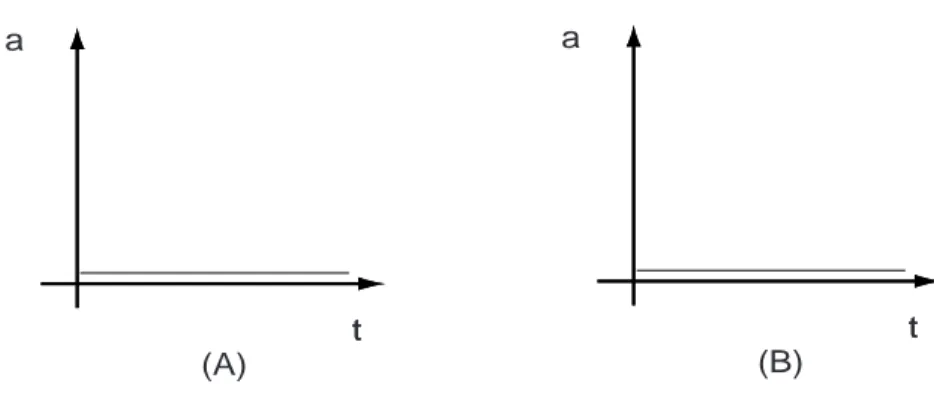
2) Air track glider moving at constant speed. Now let’s also plot an a, t graph for

1) Object standing still, 2) Object at constant speed.

Note that the the a, t graph is the slope of the v, t graph.

t a t (A) t a t (B)

(20)

1.6 Constant Acceleration: A Special Case

Velocity describes changing position and acceleration describes changing ve-locity. A quantity called jerk describes changing acceleration. However, very often the acceleration is constant, and we don’t consider jerk. When driving your car the acceleration is usually constant when you speed up or slow down or put on the brakes. (When you slow down or put on the brakes the acceleration is constant but negative and is called deceleration.) When you drop an object and it falls to the ground it also has a constant acceleration. When the acceleration is constant, then we can derive 5 very handy equations that will tell us everything about the motion. Let’s derive them and then study some examples.

We are going to use the following symbols:

t1 ≡ 0 t2 ≡ t x1 ≡ x0 x2 ≡ x v1 ≡ v0 v2 ≡ v

and acceleration a is a constant and so a1 = a2= a. Thus now

∆t = t2− t1 = t− 0 = t

∆x = x2− x1= x− x0

∆v = v2− v1 = v− v0

∆a = a2− a1= a− a = 0

(∆a must be zero because we are only considering constant a.)

Also, because acceleration is constant then average acceleration is always the same as instantaneous acceleration

¯

a = a

Now use the definition of average acceleration ¯ a = a = ∆v ∆t = v− v0 t− 0 = v− v0 t Thus at = v− v0 or

(21)

1.6. CONSTANT ACCELERATION: A SPECIAL CASE 21

v = v0+ at

(1.5) which is the first of our constant acceleration equations. If you plot this on a v, t graph, then it is a straight line for a = constant. In that case the average velocity is

¯

v = 1

2(v + v0) From the definition of average velocity

¯ v = ∆x ∆t = x− x0 t we have x− x0 t = 1 2(v + v0) = 1 2(v0+ at + v0) giving x− x0 = v0t + 1 2at 2 (1.6) which is the second of our constant acceleration equations. To get the other three constant acceleration equations, we just combine the first two.

(22)

Example Prove that v2= v2₀+ 2a(x− x0)

Solution Obviously t has been eliminated. From (1.5)

t = v− v0 a

Substituting into (1.6) gives

x− x0 = v0 µ v− v0 a ¶ + 1 2a µ v− v0 a ¶2 a(x− x0) = v0v− v02+ 1 2(v 2_{− 2vv} 0+ v20) = v2− v₀2 or v2= v2₀+ 2a(x− x0)

Example Prove that x− x0 = 1₂(v0+ v)t

Solution Obviously a has been eliminated. From (1.5)

a = v− v0 t

Substituting into (1.6) gives

x− x0 = v0t + 1 2 µ_v_{− v} 0 t ¶ t2 = v0t + 1 2(vt− v0t) = 1 2(v0+ v)t

Exercise Prove that x− x0= vt−1₂at2

(23)

1.7. ANOTHER LOOK AT CONSTANT ACCELERATION 23

1.7 Another Look at Constant Acceleration

(This section is only for students who have studied integral calculus.) The constant acceleration equations can be derived from integral calculus as follows.

For constant acceleration a6= a(x), a 6= a(t)

a = dv dt Z t2 t1 a dt = Z _dv dtdt a Z _t₂ t1 dt = Z _v₂ v1 dv a(t2− t1) = v2− v1 a(t− 0) = v − v0 v = v0+ at v = dx dt Z v dt = Z _dx dtdt

v changes ... cannot take outside integral

actually v(t) = v0+ at Z _t₂ t1 (v0+ at)dt = Z _x₂ x1 dx · v0t + 1 2at 2 ¸t2 t1 = x2− x1 = v0(t2− t1) + 1 2a(t2− t1) 2_{= x}_{− x} 0 = v0(t− 0) + 1 2a(t− 0) 2 = v0t + 1 2at 2 _{... x − x} 0= v0t +1₂at2 a = dv dt = dv dx dx dt = v dv dx

(24)

Z x2 x1 a dx = Z vdv dxdx a Z _x₂ x1 dx = Z _v₂ v1 v dv a(x2− x1) = ·₁ 2v 2 ¸v2 v1 = 1 2 ³ v₂2− v2₁´ a(x− x0) = 1 2 ³ v2− v2₀´ v2= v2₀+ 2a(x− x0)

One can now get the other equations using algebra.

1.8 Free-Fall Acceleration

If we neglect air resistance, then all falling objects have same acceleration

a =−g = −9.8 m/sec2

(g = 9.8 m/sec2).

LECTURE DEMONSTRATION: 1) Feather and penny in vacuum tube

2) Drop a cup filled with water which has a hole in the bottom. Water leaks out if the cup is held stationary. Water does not leak out if the cup is dropped.

(25)

1.8. FREE-FALL ACCELERATION 25

Carefully study Sample Problems 2-9, 2-10, 2-11. [from Halliday]

Example I drop a ball from a height H, with what speed does

it hit the ground ? Check that the units are correct.

Solution v2= v₀2+ 2a(x− x0) v0 = 0 a = −g = −9.8 m/sec2 x0 = 0 x = H v2 = 0− 2 × g (0 − −H) v =p2gH Check units:

The units of g are m sec−2 and H is in m. Thus√2gH has units of √m sec−2 m =√m2 _sec−2 _{= m sec}−1_{. which is the correct}

(26)

HISTORICAL NOTE

The constant acceleration equations were first discovered by Galileo Galilei (1564 - 1642). Galileo is widely regarded as the “father of modern science” because he was really the first person who went out and actually did expreiments to arrive at facts about nature, rather than relying solely on philosophical argument. Galileo wrote two famous books entitled Dialogues

concerning Two New Sciences [Macmillan, New York, 1933; QC 123.G13]

and Dialogue concerning the Two Chief World Systems [QB 41.G1356]. In Two New Sciences we find the following [Pg. 173]:

“THEOREM I, PROPOSITION I : The time in which any space is traversed by a body starting from rest and uniformly accel-erated is equal to the time in which that same space would be traversed by the same body moving at a unifrom speed whose value is the mean of the highest speed and the speed just before acceleration began.”

In other words this is Galileo’s statement of our equation

x− x0 =

1

2(v0+ v)t (1.7) We also find [Pg. 174]:

“THEOREM II, PROPOSITION II : The spaces described by a falling body from rest with a uniformly accelerated motion are to each other as the squares of the time intervals employed in traversing these distances.”

This is Galileo’s statement of

x− x0 = v0t + 1 2at 2_{= vt}₋1 2at 2 _(1.8)

Galileo was able to test this equation with the simple device shown in Figure 2.3. By the way, Galileo also invented the astronomical telescope !

(27)

1.8. FREE-FALL ACCELERATION 27

moveable fret wires

FIGURE 2.3 Galileo’s apparatus for verifying the constant acceleration equations.

[from “From Quarks to the Cosmos” Leon M. Lederman and David N. Schramm (Scientific American Library, New York, 1989) QB43.2.L43

(28)

1.9 Problems

1. The following functions give the position as a function of time: i) x = A

ii) x = Bt iii) x = Ct2 iv) x = D cos ωt

v) x = E sin ωt

where A, B, C, D, E, ω are constants. A) What are the units for A, B, C, D, E, ω?

B) Write down the velocity and acceleration equations as a function of time. Indicate for what functions the acceleration is constant.

C) Sketch graphs of x, v, a as a function of time.

2. The figures below show position-time graphs. Sketch the correspond-ing velocity-time and acceleration-time graphs.

t x t x t x

3. If you drop an object from a height H above the ground, work out a formula for the speed with which the object hits the ground.

4. A car is travelling at constant speed v1 and passes a second car moving

at speed v2. The instant it passes, the driver of the second car decides

to try to catch up to the first car, by stepping on the gas pedal and moving at acceleration a. Derive a formula for how long it takes to

(29)

1.9. PROBLEMS 29 catch up. (The first car travels at constant speed v1 and does not

accelerate.)

5. If you start your car from rest and accelerate to 30mph in 10 seconds, what is your acceleration in mph per sec and in miles per hour2 ? 6. If you throw a ball up vertically at speed V , with what speed does it

return to the ground ? Prove your answer using the constant acceler-ation equacceler-ations, and neglect air resistance.

(30)

(31)

Chapter 2

VECTORS

(32)

2.1 Vectors and Scalars

When we considered 1-dimensional motion in the last chapter we only had two directions to worry about, namely motion to the Right or motion to the Left and we indicated direction with a + or − sign. We found that the following quantities had a direction (i.e. could take a + or − sign):

displacement, velocity and acceleration. Quantities that don’t have a sign

were distance, speed and magnitude of acceleration.

Now in 2 and 3 dimensions we need more than a + or − sign. That’s where vectors come in.

Vectors are quantities with both magnitude and direction. Scalars are quantities with magnitude only.

Examples of Vectors are: displacement, velocity, acceleration, force, momentum, electric field

Examples of Scalars are: distance, speed, magnitude of acceler-ation, time, temperature

Before delving into vectors consider the following problem.

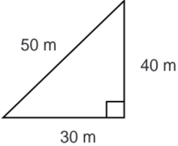
Example Joe and Mary are rowing a boat across a river which

is 40 m wide. They row in a direction perpendicular to the bank. However the river is flowing downstream and by the time they reach the other side, they end up 30 m downstream from their starting point. Over what total distance did the boat travel?

Solution Obviously the way to do this is with the triangle in

Fig. 3.1, and we deduce that the distance is 50 m.

30 m

40 m 50 m

(33)

2.2. ADDING VECTORS: GRAPHICAL METHOD 33

2.2 Adding Vectors: Graphical Method

Another way to think about the previous problem is with vectors, which are little arrows whose orientation specifies direction and whose length specifies magnitude. The displacement along the river is represented as

FIGURE 3.2 Displacement along the river.

with a length of 30 m, denoted as ~A and the displacement across the river,

denoted B,

FIGURE 3.3 Displacement across the river.

with length of 40 m. To re-construct the previous triangle, the vectors are added head-to-tail as in Fig. 3.4.

(34)

The resultant vector, denoted ~C, is obtained by filling in the triangle.

Math-ematically we write ~C = ~A + ~B.

The graphical method of solving our original problem is to take out a ruler and actually measure the length of the resultant vector ~C. You would

find it to be 50 m.

Summary: When adding any two vectors ~A and ~B, we add them head-to-tail.

Students should read the textbook to obtain more details about using the graphical method.

2.3 Vectors and Their Components

The graphical method requires the use of a ruler and protractor for measur-ing the lengths of vectors and their angles. Thus there is always the problem of inaccuracy in making these measurements. It’s better to use analytical methods which rely on pure calculation. To learn this we must learn about components. To do this we need trigonometry.

2.3.1 Review of Trigonometry

Lines are made by connecting two points. Triangles are made by connecting three points. Of all the vast number of different possible triangles, the subject of trigonometry has to do with only a certain, special type of triangle and that is a right-angled triangle, i.e. a triangle where one of the angles is 90◦. Let’s draw one:

Hypotenuse

(35)

2.3. VECTORS AND THEIR COMPONENTS 35 The side opposite the right angle is always called the Hypotenuse. Consider one of the other angles, say θ.

Hypotenuse

Adjacent Opposite

θ

FIGURE 3.6 Right-angled triangle showing sides Opposite and Adjacent

to the angle θ.

The side adjacent to θ is called Adjacent and the side opposite θ is called Opposite. Now consider the other angle α. The Opposite and Adjacent sides are switched because the angle is different.

Hypotenuse

Opposite Adjacent

α

FIGURE 3.7 Right-angled triangle showing sides Opposite and Adjacent

to the angle α.

Let’s label Hypotenuse as H, Opposite as O and Adjacent as A. Pythago-ras’ theorem states

(36)

This is true no matter how the Opposite and Adjacent sides are labelled, i.e. if Opposite and Adjacent are interchanged, it doesn’t matter for Pythagoras’ theorem.

Often we are interested in dividing one side by another. Some possible combinations are _HO, _HA, O_A. These special ratios are given special names. _HO is called Sine. A_H is called Cosine. O_A is called Tangent. Remember them by writing SOH, CAH, TOA.

Example Using the previous triangle for the river problem,

write down Sine θ, Cosine θ, Tangent θ Sine α, Cosine α, Tan-gent α Solution Sine θ = O H = 40m 50m = 4 5 = 0.8 Cosine θ = A H = 30m 50m = 3 5 = 0.6 Tangent θ = O A = 40m 30m = 4 3 = 1.33 Sine α = O H = 30m 50m = 3 5 = 0.6 Cosine α = A H = 40m 50m = 4 5 = 0.8 Tangent α = O A = 30m 40m = 3 4 = 0.75 30 m 40 m 50 m α θ

(37)

2.3. VECTORS AND THEIR COMPONENTS 37 Now whenever the Sine of an angle is 0.8 the angle is always 53.1◦. Thus

θ = 53.1◦. Again whenever Tangent of an angle is 0.75 the angle is always 36.9◦. So if we have calculated any of the ratios, Sine, Cosine or Tangent then we always know what the corresponding angle is.

2.3.2 Components of Vectors

An arbitrary vector has both x and y components. These are like shadows on the x and y areas, as shown in Figure 3.9.

x

y

A

_x

A

_y

_A

FIGURE 3.9 Components, Ax and Ay, of vector ~A.

The components are denoted Ax and Ay and are obtained by dropping a

perpendicular line from the vector to the x and y axes. That’s why we consider trigonometry and right-angled triangles!

A physical understanding of components can be obtained. Pull a cart with a rope at some angle to the ground, as shown in Fig. 3.11. The cart will move with a certain acceleration, determined not by the force ~F , but by the component Fx in the x direction. If you change the angle, the acceleration

(38)

LECTURE DEMONSTRATION of Fig. 3.10:

F

_x

FIGURE 3.10 Pulling a cart with a force ~F .

Let’s re-draw Figure 3.10, writing ~A instead of ~F as follows:

A

_x

A

_y

θ

α

(39)

2.4. UNIT VECTORS 39 Let’s denote the magnitude or length of ~A simply as A. Thus Pythagoras’

theorem gives A2 = A2_x+ A2_y and also tan θ = Ay Ax and tan α = Ax Ay (Also sin θ = Ay A, cos θ = Ax A, sin α = Ax A, cos α = Ay A)

Thus if we have the components, Axand Ay we can always get the

mag-nitude and direction of the vector, namely A and θ (or α). Similarly if we

start with A and θ (or α) we can always find Ax and Ay.

do Sample Problem 3-3 in Lecture

2.4 Unit Vectors

A vector is completely specified by writing down magnitude and direction (i.e. A and θ) x and y components (Ax and Ay).

There’s another very useful and compact way to write vectors and that is by using unit vectors. The unit vector ˆi is defined to always have a length of 1 and to always lie in the positive x direction, as in Fig. 3.12. (The symbol

∧ is used to denote these unit vectors.)

x

y

i

(40)

Similarly the unit vector ˆj is defined to always have a length of 1 also but

to lie entirely in the positive y direction.

x

y

j

FIGURE 3.13 Unit vector ˆj.

The unit vector ˆk lies in the psoitive z direction.

x

y

k

z

FIGURE 3.14 Unit vector ˆk.

Thus any arbitrary vector ~A is now written as ~

A = Axˆi + Ayˆj + Azkˆ

(41)

2.5. ADDING VECTORS BY COMPONENTS 41

2.5 Adding Vectors by Components

Finally we will now see the use of components and unit vectors. Remember

how we discussed adding vectors graphically using a ruler and protractor. A better method is with the use of components, because then we can get our answers by pure calculation.

In Fig. 3.16 we have shown two vectors ~A and ~B added to form ~C, but

we have also indicated all the components.

Ax

Cx

Ay

Bx

By

Cy

B

C

A

x

y

FIGURE 3.15 Adding vectors by components.

By carefully looking at the figure you can see that

Cx = Ax+ Bx

Cy = Ay+ By

(42)

Now let’s back-track for a minute. When we write

~

C = ~A + ~B

you should say, “Wait a minute! What does the + sign mean?” We are used to adding numbers such as 5 = 3 + 2, but in the above equation ~A, ~B and

~

C are not numbers. They are these strange arrow-like objects called vectors

which are “add” by putting head-to-tail. We should really write

~

C = ~A⊕ ~B

where⊕ is a new type of “addition”, totally unlike adding numbers. However

Ax, Bx, Ay, By, Cx, Cy are ordinary numbers and the + sign we used

above does denote ordinary addition. Thus ~C = ~A ⊕ ~B actually means Cx = Ax + Bx and Cy = Ay + By. The statement ~C = ~A⊕ ~B is really

shorthand for two ordinary addition statements. Whenever anyone writes something like ~D = ~F + ~E it actually means two things, namely Dx = Fx+Ex

and Dy = Fy+ Ey.

All of this is much more obvious with the use of unit vectors. Write

~

A = Axî + Ayˆj and ~B = Bxî + Byˆj and ~C = Cxî + Cyˆj. Now

~

C = ~A + ~B

is simply

Cxî + Cyˆj = Axî + Ayˆj + Bxî + Byˆj

= (Ax+ Bx)ˆi + (Ay+ By)ˆj

and equating coefficients of ˆi and ˆj gives Cx = Ax+ Bx

and

(43)

2.6. VECTORS AND THE LAWS OF PHYSICS 43

Example Do the original river problem using components. Solution

~

A = 30ˆi B = 40ˆ~ j ~

C = A + ~~ B

Cxî + Cyˆj = Axî + Ayˆj + Bxî + Byˆj

Ay = 0 Bx= 0 Cxˆi + Cyˆj = 30ˆi + 40ˆj Cx = 30 Cy = 40 or Cx = Ax+ Bx= 30 + 0 = 30 Cy = Ay+ By = 0 + 40 = 40 C2 = C_x2+ C_y2 = 302+ 402 = 900 + 1600 = 2500 ... C = 50

carefully study Sample Problems 3-4, 3-5

2.6 Vectors and the Laws of Physics

2.7 Multiplying Vectors

2.7.1 The Scalar Product (often called dot product)

We know how to add vectors. Now let’s learn how to multiply them. When we add vectors we always get a new vector, namely ~c = ~a+~b. When we multiply vectors we get either a scalar or vector. There are two types of vector multiplication called scalar products or vector product. (Sometimes also called dot product or cross product).

The scalar product is defined as

~a·~b ≡ ab cos φ (2.1) where a and b are the magnitude of ~a and ~b respectively and φ is the angle between ~a and ~b. The whole quantity ~a·~b = ab cos φ is a scalar, i.e. it has magnitude only. As shown in Fig. 3-19 of Halliday the scalar product is the

(44)

product of the magnitude of one vector times the component of the other vector along the first vector.

Based on our definition (2.1) we can work out the scalar products of all of the unit vectors.

Example Evaluate î· î Solution î· î = ii cos φ

but i is the magnitude of ˆi which is 1, and the angle φ is 0◦. Thus

ˆi_{· i = 1}

Example Evaluate ˆi· ˆj Solution ˆi· ˆj = ij cos 90◦ = 0

Thus we have î·î = ˆj · ˆj = ˆk · ˆk = 1 and î· ˆj = î· ˆk = ˆj · ˆk = ˆj ·î = ˆk ·î = ˆ

k· ˆj = 0. (see Problem 38)

Now any vector can be written in terms of unit vectors as ~a = axˆi+ayˆj +

azk and ~b = bˆ xˆi + byˆj + bzˆk. Thus the scalar product of any two arbitrary

vectors is

~a·~b = ab cos φ

= (axˆi + ayˆj + azk)ˆ · (bxˆi + byˆj + bzk)ˆ

= axbx+ ayby+ azbz

Thus we have a new formula for scalar product, namely

~a·~b = axbx+ ayby+ azbz (2.2)

(see Problem 46) which has been derived from the original definition (2.1) using unit vectors.

What’s the good of all this? Well for one thing it’s now easy to figure out the angle between vectors, as the next example shows.

(45)

2.7. MULTIPLYING VECTORS 45

2.7.2 The Vector Product

In making up the definition of vector product we have to define its magnitude

and direction. The symbol for vector product is ~a×~b. Given that the result

is a vector let’s write ~c≡ ~a ×~b. The magnitude is defined as

c = ab sin φ

and the direction is defined to follow the right hand rule. (~c = thumb, ~a = forefinger, ~b = middle finger.)

(Do a few examples finding direction of cross product)

Example Evaluate ˆi× ˆj

Solution |ˆi × ˆj| = ij sin 90◦ = 1 direction same as ˆk Thus ˆi× ˆj = ˆk Example Evaluate ˆk× ˆk Solution |ˆk × ˆk| = kk sin 0 = 0 Thus ˆk× ˆk = 0 Thus we have

î_{× ˆj = ˆk} ˆ_j_{× ˆk = î} ˆ_k_{× î = ˆj} ˆ

j× î = −ˆk ˆk × ˆj = −î î × ˆk = −ˆj

and

ˆi_{× ˆi = ˆj × ˆj = ˆk × ˆk = 0}

(see Problem 39) Thus the vector product of any two arbitrary vectors is

~a×~b = (axˆi + ayˆj + azk)ˆ × (bxˆi + byˆj + bzˆk)

which gives a new formula for vector product, namely

~a×~b = (aybz− azby)ˆi + (azbx− axbz)ˆj

+(axby− aybx)ˆk

(46)

2.8 Problems

1. Calculate the angle between the vectors ~r = ˆi + 2ˆj and ~t = ˆj− ˆk.

2. Evaluate (~r + 2~t ). ~f where ~r = ˆi + 2ˆj and ~t = ˆj− ˆk and ~f = ˆi − ˆj.

3. Two vectors are defined as ~u = ˆj + ˆk and ~v = ˆi + ˆj. Evaluate:

A) ~u + ~v

B) ~u− ~v

C) ~u.~v

(47)

Chapter 3

MOTION IN 2 & 3

DIMENSIONS

SUGGESTED HOME EXPERIMENT:

Design a simple experiment which shows that the range of a projectile depends upon the angle at which it is launched. Have your experiment show that the maximum range is achieved when the launch angle is 45o.

THEMES:

1. FOOTBALL.

(48)

3.1 Moving in Two or Three Dimensions

In this chapter we will go over everything we did in Chapter 2 concerning motion, except that now the entire discussion will use the formation of vectors.

3.2 Position and Displacement

In Chapter 2 we used the coordinate x alone to denote position. However for 3-dimensions position is generally described with the position vector

~

r = xˆi + yˆj + zˆk.

Now in Chapter 2, displacement was defined as a change in position, namely displacement = ∆x = x2− x1. In 3-dimensions, displacement is defined as

the change in position vector,

displacement = ∆~r = ~r2− ~r1

= ∆xˆi + ∆yˆj + ∆zˆk

= (x2− x1)ˆi + (y2− y1)ˆj + (z2− z1)ˆk

Thus displacement is a vector.

Sample Problem 4-1

3.3 Velocity and Average Velocity

In 1-dimension, the average velocity was defined as displacement divided by time interval or ¯v≡ ∆x_∆t = x2−x1

t2−t1 . Similarly, in 3-dimensions average velocity

is defined as ¯ ~v ≡ ∆~r ∆t = ~r2− ~r1 t2− t1 = ∆xî + ∆yˆj + ∆zˆk ∆t = ∆x ∆tî + ∆y ∆tˆj + ∆z ∆tkˆ = v¯xî + ¯vyˆj + ¯vzˆk

(49)

3.4. ACCELERATION AND AVERAGE ACCELERATION 49 For 1-dimension, the instantaneous velocity, or just velocity, was defined as

v≡ dx_dt. In 3-dimensions we define velocity as

~ v ≡ d~r dt = d dt(xî + yˆj + zˆk) = dx dtî + dy dtˆj + dz dtkˆ = vxî + vyˆj + vzˆk

Thus velocity is a vector.

Point to note: The instantaneous velocity of a particle is always tangent

to the path of the particle. (carefully read about this in Halliday, pg. 55)

3.4 Acceleration and Average Acceleration

Again we follow the definitions made for 1-dimension. In 3-dimensions, the average acceleration is defined as

¯ ~a≡ ∆~v ∆t = ~ v2− ~v1 t2− t1

and acceleration (instantaneous acceleration) is defined as

~a = d~v dt

Constant Acceleration Equations

In 1-dimension, our basic definitions were ¯ v = ∆x ∆t v = dx dt ¯ a = ∆v ∆t a = dv dt

(50)

We found that if the acceleration is constant, then from these equations we can prove that

v = vo+ at v2 = v_o2+ 2a(x− xo) x− xo = vo+ v 2 t x− xo = vot + 1 2at 2 = vt−1 2at 2

which are known as the 5 constant acceleration equations. In 3-dimensions we had ¯ ~v≡ ∆~r ∆t or ¯ vxˆi + ¯vyˆj + ¯vzˆk = ∆x ∆tˆi + ∆y ∆tˆj + ∆z ∆t ˆ k or ¯ vx = ∆x ∆t, ¯vy+ ∆y ∆t, v¯z = ∆z ∆t

These 3 equations are the meaning of the first vector equation ¯~v ≡ ∆~_∆tr. Similarly ~ v≡ d~r dt or vx = dx dt, vy = dy dt, vz = dz dt Similarly ¯ ~a≡ ∆~v ∆t or ¯ ax = ∆x ∆t, ¯ay = ∆y ∆t, a¯z = ∆z ∆t and ~a≡ d~v dt or ax= dvx dt , ay = dvy dt , az= dvz dt

So we see that in 3-dimensions the equations are the same as in 1-dimension except that we have 3 sets of them; one for each 1-dimension. Thus

(51)

3.5. PROJECTILE MOTION 51 if the 3-dimensional acceleration vector ~a is now constant, then ax, ay and

az must all be constant. Thus we will have 3 sets of constant acceleration

equations, namely vx = vox+ axt v_x2 = v2_ox+ 2ax(x− xo) x− xo = vox+ vx 2 t x− xo = voxt + 1 2axt 2 = vxt− 1 2axt 2 and vy = voy + ayt v_y2 = v_oy2 + 2ay(y− yo) y− yo = voy+ vy 2 t y− yo = voyt + 1 2ayt 2 = vyt− 1 2ayt 2 and vz = voz+ azt v_z2 = v2_oz+ 2az(z− zo) z− zo = voz+ vz 2 t z− zo = vozt + 1 2azt 2 = vzt− 1 2azt 2

These 3 sets of constant acceleration equations are easy to remember. They are the same as the old ones in 1-dimension except now they have subscripts for x, y, z.

3.5 Projectile Motion

(52)

3.6 Projectile Motion Analyzed

Most motion in 3-dimensions actually only occurs in 2-dimensions. The classic example is kicking a football off the ground. It follows a 2-dimensional curve, as shown in Fig. 4.1. Thus we can ignore all motion in the z direction and just analyze the x and y directions. Also we shall ignore air resistance.

v

₀

v

₀

_x

v

₀

_y

range, R

θ

(53)

3.6. PROJECTILE MOTION ANALYZED 53

Example A football is kicked off the ground with an initial

ve-locity of ~vo at an angle θ to the ground. Write down the x

constant acceleration equation in simplified form. (Ignore air re-sistance)

Solution The x direction is easiest to deal with, because there is

no acceleration in the x direction after the ball has been kicked,

i.e. ax = 0. Thus the constant acceleration equations in the x

direction become vx = vox v2_x = v_ox2 x− xo = vox+ vx 2 t = voxt = vxt x− xo = voxt = vxt (3.1)

The first equation (vx = vox) makes perfect sense because if

ax = 0 then the speed in the x direction is constant, which

means vx = vox. The second equation just says the same thing.

If vx = vox then of course also vx2 = vox2 . In the third equation

we also use vx = vox to get vox₂+vx = vox+v₂ ox = vox or vox₂+vx = vx+vx

2 = vx. The fourth and fifth equations are also consistent

with vx = vox, and simply say that distance = speed × time

when the acceleration is 0.

Now, what is voxin terms of vo ≡ |~vo| and θ? Well, from Fig. 4.1

we see that vox = vocos θ and voy = vosin θ. Thus (3.1) becomes

(54)

Example What is the form of the y-direction constant

acceler-ation equacceler-ations from the previous example ?

Solution Can we also simplify the constant acceleration

equa-tions for the y direction? No. In the y direction the acceleration is constant ay =−g but not zero. Thus the y direction equations

don’t simplify at all, except that we know that the value of ay is

−g or −9.8 m/sec2_.

Also we can write voy = vosin θ. Thus the equations for the y

direction are vy = vosin θ− gt v2_y = (vosin θ)2− 2g(y − yo) y− yo = vosin θ + vy 2 t y− yo = vosin θ t− 1 2gt 2

An important thing to notice is that t never gets an x, y or z subscript. This is because t is the same for all 3 components, i.e. t = tx = ty = tz.

(You should do some thinking about this.) LECTURE DEMONSTRATIONS

1) Drop an object: it accerates in y direction. Air track: no acceleration in x direction.

2) Push 2 objects off table at same time. One falls in vertical path and the other on parabolic trajectory but both hit ground at same time. 3) Monkey shoot.

(55)

Example The total horizontal distance (called the Range) that a

football will travel when kicked, depends upon the initial speed and angle that it leaves the ground. Derive a formula for the Range, and show that the maximum Range occurs for θ = 45◦. (Ignore air resistance and the spin of the football.)

Solution The Range, R is just

R = x− xo = voxt

= vocos θ t

Given vo and θ we could calculate the range if we had t. We

get this the y direction equation. From the previous example we had

y− yo = vosin θ t−

1 2gt

2

But for this example, we have y− yo= 0. Thus

0 = vosin θ t− 1 2gt 2 0 = vosin θ − 1 2gt ⇒ t = 2vosin θ g

Substituting into our Range formula above gives

R = vocos θ t = 2v 2 osin θ cos θ g = v 2 osin 2θ g

using the formula sin 2θ = 2 sin θ cos θ. Now R will be largest when sin 2θ is largest which occurs when 2θ = 90o. Thus θ = 45o.

(56)

COMPUTER SIMULATION (Interactive Physics): Air Drop.

H=200 m

R=400 m

origin

FIGURE 4.2 Air Drop.

Example A rescue plane wants to drop supplies to isolated

mountain climbers on a rocky ridge a distance H below. The plane is travelling horizontally at a speed of vox. The plane

releases supplies a horizontal distance of R in advance of the mountain climbers. Derive a formula in terms of H, v0x,R and

g, for the vertical velocity (up or down) that the supplies should

be given so they land exactly at the climber’s position. If H = 200 m, v0x = 250 km/hr and R = 400m, calculate a numerical

(57)

Solution Let’s put the origin at the plane. See Fig. 4.2. The

initial speed of supplies when released is vox = +250 km/hour

x− xo = R− 0 = R

ay = −g

y− yo = 0− H = −H (note the minus sign !)

We want to find the initial vertical velocity of the supplies, namely voy. We can get this from

y− yo = voyt + 1 2ayt 2₌_−H = voyt− 1 2gt 2 or voy = −H t + 1 2gt and we get t from the x direction, namely

x− xo = voxt = R ⇒ t = R vox giving voy = −H vox R + 1 2g R vox

which is the formula we seek. Let’s now put in numbers: = −200 m× 250 km hour −1 400 m +1 29.8 m sec2 × 400 km 250 km hour−1 = −125 km hour + 7.84 m2hour sec2_km = −125 1000 m 60× 60 sec + 7.85 m2× 60 × 60 sec sec2_{1000 m} = −34.722 m/sec + 28.22 m/sec = −6.5 m/sec

Thus the supplies must be thrown in the down direction (not up) at 6.5 m/sec.

(58)

3.7 Uniform Circular Motion

In today’s world of satellites and spacecraft circular motion is very important to understand because many satellites have circular orbits. Also circular motion is a classic example where we have a definite non-zero acceleration even though the speed of a satellite is constant. This occurs because the direction of velocity is constantly changing for the satellite even though the magnitude of velocity (i.e. speed) is constant. This is shown in Fig. 4-19 of Halliday. The word “uniform” means that speed is constant.

In circular motion, there is a well defined radius which we will call r. Also the time it takes for the satellite to complete 1 orbit is called the period

T . If the speed is constant then it is given by v = ∆s

∆t = 2πr

T (3.2)

Here I have written ∆s_∆t instead of ∆x_∆t or ∆y_∆t because ∆s is the total distance

around the circle which is a mixture of x and y. 2πr_T is just the distance of 1 orbit (circumference) divided by the time of 1 orbit (period).

What about the acceleration? Well that’s just a = ∆v_∆t but how do we work it out? Look at Figure 4.3, where the displacement and velocity vectors are drawn for a satellite at two different positions P1 and P2.

= r

₂

- r

₁

∆

v = v

2 - v

1 ∆

r

₂

r

₁

v

₂

v

₁

v

1 v

₂

∆θ

∆

s

P

₁

P

₁

(59)

3.7. UNIFORM CIRCULAR MOTION 59 Now angle ∆θ is defined as (with|~r1| = |~r2| ≡ r)

∆θ ≡ ∆s

r = v∆t

r (3.3)

The velocity vectors can be re-drawn as in the bottom part of the figure. The triangle is similar to the top triangle in that the angle ∆θ is the same. Also the speed v is constant, meaning that

|~v2| = |~v1| ≡ v. (3.4)

Writing ∆v≡ |∆~v| the bottom figure also gives ∆θ = ∆v

v (3.5)

Now the magnitude of acceleration is

a = ∆v

∆t (3.6)

Combining the above two equations for ∆θ gives ∆v_∆t = v_r2, i.e.

a≡ ∆v

∆t =

v2

r (3.7)

This is a very important equation. Whenever we have uniform circular

motion we always know the actual value of acceleration if we know v and

r. We have worked out the magnitude of the acceleration. What about its

direction? I will show you a VIDEO in class (Mechanical Universe video #9 showing vectors for circular motion) which will clearly show that the direction of acceleration is always towards the center of the circle. For this reason it is called centripetal acceleration.

One final thing. When you drive your car around in a circle then you, as the driver, feel as though you are getting pushed against the door. In reality it is the car that is being accelerated around in the circle, and because of your inertia, the car pushes on you. This “acceleration” that you feel is the same as the car’s acceleration. The “acceleration” you feel is called the centrifugal acceleration. The same idea occurs when you spin-dry clothes in a washing machine.

(60)

Example Future spacecraft will be made to spin in order to

pro-vide artificial gravity for the astronauts. Suppose the spacecraft is a cylinder of L in length. Derive a formula for the rotation period would it need to spin in order to simulate the gravity on Earth. If L = 1 km what is the numerical value foe the period ?

Solution The centifugal acceleration is a and we want it to equal

g. Thus g = v 2 r = (2πr/T )2 r = 4π2_r T2 Thus T2= 4π 2_r g giving T = 2π s L g

which is the formula we seek. Putting in numbers:

T = 2π r 1000 m 9.8 m sec−2 = 2π√102.04 sec−2 = 2π× 10.1 sec = 63.5 sec i.e. about once every minute!

Example The Moon is 1/4 million miles from Earth. How fast

does the Moon travel in its orbit ?

Solution The period of the Moon is 1 month. Thus

v = 2πr T = 2π× 250, 000 miles 30× 24 hours = 2, 182 mph i.e. about 2000 mph!

(61)

3.8. PROBLEMS 61

3.8 Problems

1. A) A projectile is fired with an initial speed vo at an angle θ with

respect to the horizontal. Neglect air resistance and derive a formula for the horizontal range R, of the projectile. (Your formula should make no explicit reference to time, t). At what angle is the range a maximum ?

B) If v0 = 30 km/hour and θ = 15o calculate the numerical value of

R.

2. A projectile is fired with an initial speed vo at an angle θ with respect

to the horizontal. Neglect air resistance and derive a formula for the maximum height H, that the projectile reaches. (Your formula should make no explicit reference to time, t).

3. A) If a bulls-eye target is at a horizontal distance R away, derive an expression for the height L, which is the vertical distance above the bulls-eye that one needs to aim a rifle in order to hit the bulls-eye. Assume the bullet leaves the rifle with speed v0.

B) How much bigger is L compared to the projectile height H ? Note: In this problem use previous results found for the range R and height H, namely R = v 2 0sin 2θ g

=

2v2 0sin θ cos θ g and H = v2 0sin 2_θ 2g .

4. Normally if you wish to hit a bulls-eye some distance away you need to aim a certain distance above it, in order to account for the downward motion of the projectile. If a bulls-eye target is at a horizontal distance

D away and if you instead aim an arrow directly at the bulls-eye (i.e.

directly horiziontally), by what (downward) vertical distance would you miss the bulls-eye ?

5. Prove that the trajectory of a projectile is a parabola (neglect air resistance). Hint: the general form of a parabola is given by y =

ax2+ bx + c.

6. Even though the Earth is spinning and we all experience a centrifugal acceleration, we are not flung off the Earth due to the gravitational force. In order for us to be flung off, the Earth would have to be spinning a lot faster.

A) Derive a formula for the new rotational time of the Earth, such that a person on the equator would be flung off into space. (Take the radius of Earth to be R).

(62)

B) Using R = 6.4 million km, calculate a numerical anser to part A) and compare it to the actual rotation time of the Earth today.

7. A staellite is in a circular orbit around a planet of mass M and radius

R at an altitude of H. Derive a formula for the additional speed that

the satellite must acquire to completely escape from the planet. Check that your answer has the correct units.

8. A mass m is attached to the end of a spring with spring constant k on a frictionless horizontal surface. The mass moves in circular motion of radius R and period T . Due to the centrifugal force, the spring stretches by a certain amount x from its equilibrium position. Derive a formula for x in terms of k, R and T . Check that x has the correct units.

9. A cannon ball is fired horizontally at a speed v0 from the edge of the

top of a cliff of height H. Derive a formula for the horizontal distance (i.e. the range) that the cannon ball travels. Check that your answer has the correct units.

10. A skier starts from rest at the top of a frictionless ski slope of height

H and inclined at an angle θ to the horizontal. At the bottom of

the slope the surface changes to horizontal and has a coefficient of kinetic friction µkbetween the horizontal surface and the skis. Derive

a formula for the distance d that the skier travels on the horizontal surface before coming to a stop. (Assume that there is a constant deceleration on the horizontal surface). Check that your answer has the correct units.

11. A stone is thrown from the top of a building upward at an angle θ to the horizontal and with an initial speed of v0as shown in the figure. If

the height of the building is H, derive a formula for the time it takes the stone to hit the ground below.

(63)

3.8. PROBLEMS 63

θ

vo

(64)

Norbury John - Elementary Mechanics and Thermodynamics.pdf (1,1 MB)

ELEMENTARY

MECHANICS & THERMODYNAMICS

Professor John W. Norbury

Contents

PREFACE

INTRODUCTION - What is Physics?

Chapter 1

MOTION ALONG A

STRAIGHT LINE

1.1

Motion

1.2

Position and Displacement

1.3

Average Velocity and Average Speed

1.4

Instantaneous Velocity and Speed

1.5

Acceleration

1.6

Constant Acceleration: A Special Case

1.7

Another Look at Constant Acceleration

1.8

Free-Fall Acceleration

HISTORICAL NOTE

moveable fret wires

1.9

Problems

Chapter 2

VECTORS

2.1

Vectors and Scalars

2.2

Adding Vectors: Graphical Method

2.3

Vectors and Their Components

x

y

A

x

A

y

A

F

F

x

A

A

x

A

y

θ

α

2.4

Unit Vectors

x

y

i

x

y

j

x

y

k

z

2.5

Adding Vectors by Components

Ax

Cx

Ay

Bx

By

Cy

B

C

A

x

y

_x

_y

_A

_x

_x

_y

₀

₀

_x

₀

_y

₂

₁

₂

₁

₂

₁

₂

₁