2021-01-20T14:52:00Z
Acceptance in OA@INAF
Anomalous Microwave Emission in HII Regions: Is it Really Anomalous? The Case
of RCW 49
Title
Paladini, R.; INGALLINERA, Adriano; Agliozzo, C.; Tibbs, C.T.; Noriega-Crespo,
A.; et al.
Authors
10.1088/0004-637X/813/1/24
DOI
http://hdl.handle.net/20.500.12386/29880
Handle
THE ASTROPHYSICAL JOURNAL
Journal
813
ANOMALOUS MICROWAVE EMISSION IN H
IIREGIONS: IS IT REALLY ANOMALOUS? THE CASE OF
RCW 49
Roberta Paladini1, Adriano Ingallinera2, Claudia Agliozzo2,3, Christopher T. Tibbs4, Alberto Noriega-Crespo5, Grazia Umana2, Clive Dickinson6, and Corrado Trigilio2
1
Infrared Processing Analysis Center, California Institute of Technology, 770 South Wilson Ave., Pasadena, CA 91125, USA 2
Osservatorio Astrofisico di Catania, Via S. Sofia 78, I-95123 Catania Italy 3
Departamento de Ciencias Fisicas, Universidad Andres Bello, Avda. Republica 252, Santiago 8320000, Chile 4
Scientific Support Office, Directorate of Science and Robotic Exploration,European Space Research and Technology Centre (ESA/ESTEC), Keplerlaan 1, 2201 AZ, Noordwijk, The Netherlands
5
Space Telescope Science Institute, 3700 San Martin Drive, Baltimore, MD 21218, USA 6
Jodrell Bank Centre for Astrophysics, Alan Turing Building, School of Physics & Astronomy, The University of Manchester, Oxford Road, Manchester M13 9PL, UK
Received 2015 April 4; accepted 2015 September 11; published 2015 October 22
ABSTRACT
The detection of an excess of emission at microwave frequencies with respect to the predicted free–free emission has been reported for several Galactic HIIregions. Here, we investigate the case of RCW 49, for which the Cosmic
Background Imager tentatively (∼3σ) detected Anomalous Microwave Emission (AME) at 31 GHz on angular scales of 7′. Using the Australia Telescope Compact Array, we carried out a multi-frequency (5, 19, and 34 GHz) continuum study of the region, complemented by observations of the H109α radio recombination line. The analysis shows that:(1) the spatial correlation between the microwave and IR emission persists on angular scales from 3 4 to 0 4, although the degree of the correlation slightly decreases at higher frequencies and on smaller angular scales;(2) the spectral indices between 1.4 and 5 GHz are globally in agreement with optically thin free– free emission, however, ∼30% of these are positive and much greater than −0.1, consistent with a stellar wind scenario; and(3) no major evidence for inverted free–free radiation is found, indicating that this is likely not the cause of the Anomalous Emission in RCW 49. Although our results cannot rule out the spinning dust hypothesis to explain the tentative detection of AME in RCW 49, they emphasize the complexity of astronomical sources that are very well known and studied, such as HIIregions, and suggest that, at least in these objects, the reported excess of
emission might be ascribed to alternative mechanisms such as stellar winds and shocks. Key words: dust, extinction– HIIregions– radio continuum: ISM – radio lines: ISM
1. INTRODUCTION
Studies in recent years have brought direct evidence that an additional component of emission is present both in the diffuse Interstellar Medium (ISM; e.g., Davies et al. 2006) and in
individual sources on or close to the Galactic Plane (e.g., Planck Collaboration XX 2011; Planck Collaboration Int. XV 2014). This component manifests itself in the microwave
regime (10–60 GHz) and is often denoted with the term anomalous, as it appears to be closely correlated with infrared (IR) data, therefore suggesting a possible association with dust, despite exhibiting a pronounced excess with respect to the predicted thermal vibrational dust emission at these frequen-cies. Draine & Lazarian(1998) have proposed that very small
rotating dust grains (Polycyclic Aromatic Hydrocarbons, i.e., PAHs, or Very Small Grains, i.e., VSGs) are responsible for the observed microwave excess.
The Cosmic Background Imager (hereafter CBI, Padin et al.2002), observing the sky at 31 GHz and with a synthetic
beam of ∼6 8, detected anomalous microwave emission (AME) at a 3.3σ level in the HIIregion RCW 49 (Dickinson
et al.2007). The prediction of free–free emission for the source
was based on a power-law fit of continuum data in the range 2.7–15 GHz, providing an expected 31 GHz flux of 99.6 ± 13.4 Jy, i.e., much lower than the flux measured by CBI of 146.5± 5.2 Jy. Signatures of AME were also reported by CBI for RCW 175 which, with a 14.3σ detection (Dickinson et al.
2009; Tibbs et al. 2012; Battistelli et al. 2015), represents to
date the best example of microwave excess emission in an HII
region, as well as for six other southern HIIregions, and by the
Very Small Array (VSA) in nine HII regions in the northern
hemisphere(Todorovic et al.2010).7Despite these claims for a detection, the observational scenario appears far from clear: a sample of 16 HII regions observed by Scaife et al. (2008)
showed no statistically significant excess, and the original claim of an AME detection in the HIIregion LPH+201.6+1.6
(Finkbeiner et al. 2002) was later revised by CBI (Dickinson
et al.2006) and VSA measurements (Scaife et al.2007).
In general, the possibility of detecting AME in HIIregions is
very intriguing from a theoretical point of view. On one side, HII regions are ideal candidates to harbor this emission, as
processes common to this type of environment, such as plasma drag and photoelectric effect, can generate enough angular momentum to spin the grains and induce detectable microwave radiation. However, significant dust grain depletion is expected to occur in HII regions as a consequence of the intense
radiation pressure and stellar winds(Inoue2002; Draine2011).
Even more importantly, embedded optically thick Ultra Compact HII (UCHII) regions could mimic, in this case, an
excess at microwave frequencies. In fact UCHII regions are
characterized by high emission meaures (i.e., 109–10pc cm−6) and by self-absorbed free–free emission at frequencies up to several GHz. This self-absorbed free–free could potentially generate the observed rising spectrum attributed to AME.
The Astrophysical Journal,813:24(12pp), 2015 November 1 doi:10.1088/0004-637X/813/1/24
© 2015. The American Astronomical Society. All rights reserved.
7 For a comprehensive summary of AME observations in H
II regions, we refer the reader to Dickinson(2013).
Motivated by this complex scenario, in 2008 we requested Australia Telescope Compact Array (ATCA) high-resolution observations of RCW 49. The goal of the observations was to follow-up on the original CBI detection, in order to shed light on the nature of the reported microwave excess.
RCW 49, located at(R.A., decl.) = (10h24m14 6,−57°46′ 58″), is the most luminous and massive HII region of the
southern Galaxy(e.g., Paladini et al.2003), with a bolometric
luminosity of 1.4× 10⁷Leand a stellar mass of∼3 × 10⁴Me (Vacca et al. 1996). The source has an estimated age of
2–3 Myr (Piatti et al. 1998), while its distance remains
uncertain, with different authors suggesting a distance any-where between 2.3 (e.g., Brand & Blitz 1993) and 6–7 kpc
(e.g., Benaglia et al. 2013). RCW 49 extends for ∼2° and is
characterized by a very complex morphology. At its center is the Westerlund 2 (Wd2, Westerlund 1960) compact cluster,
comprising a dozen OB stars. An additional set of about 30 new OB star candidates is found in and around Wd2. Beyond the cluster core there are three more massive stars, i.e., a star of spectral type O4 or O5 (Rauw et al. 2007), a binary Wolf–
Rayet star, WR20a, which is the most massive binary system in the Galaxy with a well-determined mass (Rauw et al. 2005),
and another Wolf–Rayet star, WR20b (van der Hucht 2001),
situated several arcminutes away.
RCW 49 has been extensively investigated at both radio and IR wavelengths. In the radio continuum, data are available at 408 MHz(73 cm, Shaver & Goss1970b), 2.7 GHz (11 cm, Day
et al. 1972), 5 GHz (6 cm, Caswell & Haynes 1987), 8.7 GHz
(3.4 cm, McGee et al. 1975) and 14.7 GHz (2 cm, McGee &
Newton 1981). All these observations are characterized by
angular resolutions ranging from 8 2 (at 2.7 GHz) to ∼2′ (e.g 14.7 GHz). The Molonglo Observatory Synthesis Telescope carried out sub-arcmin resolution observations at 0.843 GHz (35.6 cm, Whiteoak et al.1989), and more recently the ATCA
targeted the core of RCW 49 at 1.4 and 2.4 GHz (21 and 12.5 cm, Whiteoak & Uchida1997, hereafter WU97), as well
as at 5.5 and 9.0 GHz (5.4 and 3.3 cm, Benaglia et al. 2013).
These observations span angular resolutions from 10″ to 2″. All these data show that the core of RCW 49 is dominated by a two-shell system, the larger(7 3 in diameter) and more massive of which is located to the east and is centered on the Wd2 cluster, while the second shell(4 1 in diameter), located to the west, surrounds WR20B.
At shorter wavelengths, RCW 49 has been observed with the Spitzer Telescope by IRAC, as part of the GLIMPSE survey (Benjamin et al. 2003), and by MIPS (PI. J. Houck, pid 63).
These combined observations provide information in five photometric bands, from 3.6 to 24μm (i.e., 3.6, 4.5, 5.6, 8, and 24μm), with a spatial resolution from 2″ to 6″. We note that only partial data exist at 24μm, due to hard saturation in the bright core of the source. A comprehensive analysis of the GLIMPSE data for the region is provided in Whitney et al. (2004). This area of the sky was also covered by the Wide-field
Infrared Survey Explorer (WISE; Wright et al. 2010) all-sky
survey at 3.4, 4.6, 12 and 22μm, with spatial resolution from 6″ to 12″. As in the case of GLIMPSE, severe saturation of the core of RCW 49 occurs at 22μm. Finally, RCW 49 was targeted by dedicated Herschel (Pilbratt et al. 2010) PACS
(70 μm and 160 μm, at 6″ and 12″, respectively) and SPIRE (250 μm, 350 μm, 500 μm, at 18″, 25″ and 35″, respectively) Cycle 2 Open Time parallel mode observations (PI. R. Paladini). The analysis of these Herschel data will be the
subject of a forthcoming publication(R. Paladini et al. 2015, in preparation).
Noticeably, the brightest emission, at both radio and IR wavelengths, is found in correspondence of the ridge located between the two shells(see Figure1).
The paper is organized as follows. In Section2we describe the new ATCA continuum and radio recombination line(RRL) observations of the core of RCW 49. In Section3we provide details on the data reduction. In Section4we analyze this new data set. Finally, we discuss our results in Section 5, and present the conclusions in Section6.
2. ATCA OBSERVATIONS
With the ATCA multi-frequency high-resolution observa-tions, we intended to achieve three main objectives:
(1) search for a spatial correlation of the radio continuum emission with dust emission, and study its dependence on frequency;(2) generate a spectral index map to investigate the nature of the physical mechanism responsible for the observed microwave excess; and(3) verify the possibility that the AME deteted by the CBI experiment is due to optically thick free– free emission associated with UCHIIregions. For (1) and (2)
we needed continuum data, while point(3) can be addressed by means of RRL observations.
To this end, we requested observing time at four different frequencies(5, 18/19, 22, and 34 GHz) and in different array configurations (750-m/1.5-km, 1.5-km/EW 352 and EW 352). At 5 GHz, we observed simultaneously the continuum and the H109α line, whose rest-frame frequency is 5.0089 GHz. Table1 provides a summary of the observations. Due to bad weather conditions, the 22 GHz data are of poor quality. Therefore, these data were not included in our analysis and are omitted in Tables2and 3.
The CBI observations covered an area which extends 7 8 × 5 6 and is centered on (R.A., decl.) = (10h24m20s, −57°44′57″). This area corresponds to the west shell, comprising the WR20b cluster and the ridge (see Figure 1).
The ATCA observations were designed to overlap with the CBI observations. The 18/19 and 34 GHz observations were carried out in mosaic mode (with 49 pointings at 19 GHz and 63 pointings at 34 GHz), and using a 128 MHz bandwidth, to allow an adequate sampling of the continuum emission. The area mapped at 18/19 GHz covers the same field of view of the 5 GHz data while, due to partially adverse weather conditions during the observational campaign, the area mapped at 34 GHz covers only the region of the ridge and its immediate surroundings. To observe the H109α line, we used a 16 MHz bandwith with 512 channels, which provides a spectral channel resolution of 1.875 km s−1.
3. DATA REDUCTION
In this section we describe the generation of the 5, 19, and 34 GHz maps displayed in Figures2–4, and the extraction of the H109α line shown in Figure5.
3.1. Radio Continuum Data
The MIRIAD software (Sault et al. 1995)8 was used to perform the standard calibration steps, which include: (1) flagging corrupted data, spikes and baselines; (2) performing
8
bandpass calibration;(3) removing bad channels; (4) improving bandpass solutions; (5) determining time-based antenna gains by interpolation between scans taken on the phase calibrator; and(6) flux-density bootstrapping. A complete list of bandpass,
flux, and phase calibration sources is provided in Table2. In total, no more than 3%–5% of the data were flagged.
At 5 GHz, in order to achieve the best uv-coverage, as well as the best signal-to-noise ratio, we concatenated the data sets obtained in the 750 B and 1.5 C configurations. We also concatenated the 18 and 19 GHz data sets, as we do not expect any significant changes in the spectral index between these two frequencies. Hereafter we will only discuss results on the combined,final images.
The imaging process was carried out with CASA9v3.3. For all frequencies, with the exception of 5 GHz, we used a Briggs
Figure 1. 31 GHz CBI contours overlaid on a composite three-color image of RCW 49: IRAC 3.6 μm (blue) and 8 μm (green) from the GLIMPSE survey, PACS 160μm (red) from the Herschel OT2 program “Unveiling the mysterious case of RCW 49: a powerful HIIregion with associated Anomalous Microwave Emission” (PI.: R. Paladini). The IRAC 3.6 μm band shows the stellar content of the region, including the bright WR20b and Westerlund 2 cluster. The 8 μm band is dominated by the 7.7μm PAH feature, and it highlights the Photo Dissociation Region (PDR) associated with RCW 49. Finally, the PACS 160 μm data indicate the presence of cold dust, both in the PDR and in its surroundings.
Table 1 Observations Summary
Observation Date ATCA Configuration Central Wavelength Central Frequency Bandwidth Integration Time
(cm) (GHz) (MHz) (hr) 2008 Dec 14–15 750 B 5.99 5.0089 16 10.9 2009 Jan 23–24 1.5 C 5.99 5.0089 16 10.4 2009 Jan 25 EW 352 1.35 22.2350a 8 10.1 2009 Feb 7–8 EW 352 0.87 34.5600 128 10.1 2009 Feb 8–9 EW 352 1.62+ 1.54 18.4960+ 19.5200 128 10.4 Note. a
These data were not used for the analysis. See the text for more details. Table 2 List of Calibrators Calibrator Type 5 GHz 19 GHz 34 GHz Bandpass 1934–638 0537–441 0537–441 Flux 1934–638 1934–638 1934–638 Phase 1036–52 1045–62 1045–62 9 http://casa.nrao.edu 3
weighting, which allows a good match between noise and resolution. The parameter robust was set to zero, to minimize sidelobe contributions from bright sources. At 5 GHz, we used a natural weighting scheme, in order to assign more weight to the shortest spatial frequencies, and achieve a better sensitivity at the largest angular scales. Deconvolution of the dirty images was performed by default with the Clark algorithm. Alternatively, the Högbom algorithm was used when the uv-coverage was too poor for imaging. In addition, a correction for the primary beam was applied. Table3provides the synthetic beams, peakflux densities, and noise of the final maps, shown in Figures2–4.
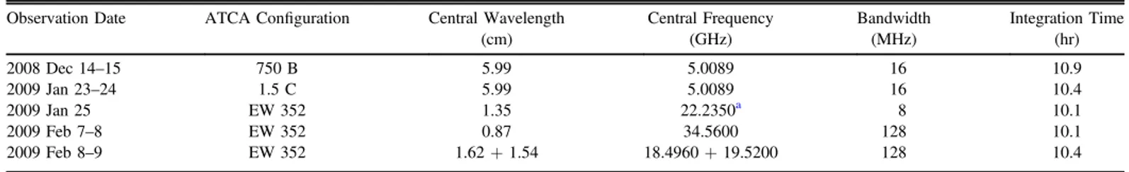
At 5 GHz, the map shows the ridge plus two-shell system already revealed by previous cm observations. However, the east shell is only partially contained in the field of view. The ridge and the west shell are also visible at 19 GHz. At this frequency, the circular shell structure appears almost complete, with the exception of an opening toward the east. Both the 5 and 19 GHz maps present filament-like structures, as well as regions of increased emission along the ridge and on the
southern part of the west shell. These knots are rather compact and their size is typically of the order of 10″. Similar knots also characterize the map at 34 GHz. Noteworthy, the 5 and 19/34 GHz maps reveal morphological differences in correspondence of the ridge. In particular, at 19 and 34 GHz the maps present a few emission features which are either completely absent or only barely visible in the 5 GHz map, despite the fact that the size of these features is compatible with the range of angular scales which the 5 GHz map is sensitive to. For instance, the spur centered at(R.A., decl.) = (10h24m16 2, −57°45′02″), roughly 40″ in size, is quite prominent and diffuse at 19 and 34 GHz, while it is rather faint and filamentary at 5 GHz (see Figures 2–4). Likewise, the feature
at(R.A., decl.) = (10h24m18 0,−57°46′45 05), ∼25″ long, is again bright and extended at 19/34 GHz, but virtually invisible at 5 GHz (see Figures 2–4). Such differences might be
indicative of rising spectral indices or of an additional component of emission at high frequency. At the same time, they could be ascribed, at least in part, to the sensitivity to different angular scales of the individual data sets.
Table 3 ATCA Datasets
Frequency Synthetic Beam Imax rms θmin θmax
(GHz) (arcsec) (mJy beam−1) (mJy beam−1) (arcsec) (arcmin)
5 7.3× 7.3 288.7 4.9 2.7 3.4
19 8.5× 6.1 175.4 1.2 0.7 1.7
34 8.3× 4.2 28.4 1.1 0.4 1
Note. The parameters listed above for the 5 GHz map refer to the original data set, i.e., prior to filtering in the uv-plane (see Section4.2). θminandθmaxindicate,
respectively, the smallest and largest imaged angular scales.
Figure 3. ATCA 19 GHz image of RCW49. The synthetic beam is shown in the bottom right corner. The beam PA is −12°.3. The map units are Jy beam−1.
Figure 4. ATCA 34 GHz image of RCW49. The synthetic beam is shown in the top left corner. The beam PA is 160°.2. The map units are Jy beam−1.
5
3.2. Recombination Line Data
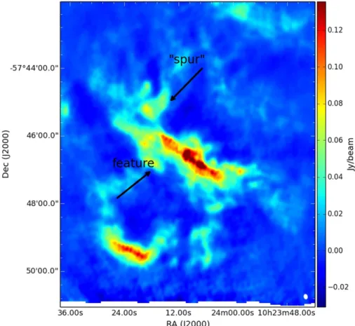
As mentioned in the previous section, the recombination line and continuum observations were performed simultaneously, thus covering the same 7 8× 5 6 area of the sky. The 5 GHz recombination line data set was reduced again using CASA v3.3. The average noise level per channel was estimated to be of the order of ∼2.6 mJy beam−1. Accordingly, line emission was found only at three positions (denoted as “A,” “B,” “C”) located along the ridge(see Figure2). We detected no emission
in the inner part of the west shell.
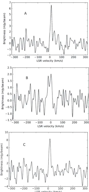
Using the task viewer, we extracted a cumulative spectrum within a box of the same size of the synthetic beam(∼7″) and centered at each position. In our system configuration we had a continuum bandwidth of 13 MHz, which allowed us to estimate the continuum level, TC, byfitting the data, minus the line, with a power-law model. A Gaussian fit was applied to the continuum-subtracted data(see Figure5). Both the continuum
and the linefits were carried out with the MATLAB fitting tool (cftool). The Gaussian fit to the line gives the line peak temperature, TL, central velocity, V, and width to half-intensity, ΔV (see Table4).
We estimated the probability of a false detection. From Table4, the statistical significance of the H109α line is ∼3σ in region A and B, and∼2σ in region C, which corresponds to a probability of a spurious detection in a single velocity channel of, respectively, 1/370 and 1/50. Therefore, the probability that at least one out of N velocity channels has an S/N of 3 (or 2) is given by 1–(1–1/370)N(or 1–(1–1/50)N). Since we apply the positivity condition,10the previous expression becomes 1– (1–1/740)N (or 1–(1–1/100)N). We now consider the number of velocity channels that are effectively used for the detection of the line. First of all, the channels at the edge of bandwidth are discarded, as they are too noisy to provide any useful information. This operation brings the number N of channels from 512 to 400. In addition, we restrict the search of the line to the velocity range +/−30 km s−1, which is the range of velocities compatible with the position of RCW 49 in the l-v diagram (see Figure 2 of Furukawa et al.2009). This further
decreases N from 400 to roughly 40 channels. Following these considerations, wefinally estimate that the probability that the lines in region A and B are spurious is 1–(1–1/740)40∼ 0.05, while for region C is 1–(1–1/100)40∼ 0.33. This calculation shows that our detections, especially in region C, are only marginal.
From the recombination lines, we computed the electron temperature, Te, by applying the 5 GHz specific relation (Caswell & Haynes 1987)
T T V T 10, 150 K. 1 e L C 0.87 ( ) = D -⎛ ⎝ ⎜ ⎞ ⎠ ⎟
The expression above is an approximation of the Shaver et al.(1983) formula (see their Equation (1)), with ν = 5 GHz
and where we assume LTE conditions and that the fraction of ionized He is negligible(ne=nH+).
The emission measure, EM, is defined as
n dl
EM pc cm 2
0 e
2 6 ( )
ò
= ¥ - and it is derived from the 5-GHz continuum measurement. In
fact, in the optically thin regime
TC=Te
(
1-e-tC)
Te Ct K, ( )3Figure 5. Cumulative continuum-subtracted spectra extracted from positions “A” (top panel), “B” (middle panel), and “C” (bottom panel). The spectra have been smooothed using a 10-channel Hanningfilter. The H109α line is centered on the LSR V∼ 0 km s−1.
10
The positivity condition states that an emission line—such as a RRL— always consists in a positive signal, while a noise spike can be both positive or negative.
Table 4
Recombination Line Parameters
Region R.A. Decl. TL TC rms SNR ΔV V Te EM ne
h m s d m s (mJy beam−1) (mJy beam−1) (mJy beam−1) (km s−1) (km s−1) (K) (pc cm−6) (cm−3)
A 10 24 15.1 −57 46 10 6.94 33.24 2.3 3.04 9.2± 2.6 16.0± 1.8 5750± 1960 170± 98 13.0± 3.8 B 10 24 07.0 −57 46 52 4.26 21.80 1.6 2.71 3.1± 1.0 −2.6 ± 5.5 15700± 8430 159± 144 12.6± 5.7 C 10 24 13.6 −57 46 13 8.79 36.90 3.9 2.28 12.4± 2.5 16.0± 1.8 3955± 1110 166± 80 12.9± 3.1 7 The Astrophysical Journal, 813:24 (12pp ), 2015 November 1 Pa ladini et al.
with τC, the optical thickness for the continuum emission, given by T 8.24 10 GHz EM. 4 C 2 e1.35 2.1 · ( ) t = - - ⎜⎛ n ⎟ -⎝ ⎞⎠
From Equation(2), if neis constant, it also follows that
n
l
EM
cm , 5
e -3 ( )
with l as the linear size of the emitting region. Table4provides the derived values of Te, EM and ne by taking l = 1 pc. Uncertainties on these quantities were obtained by propagating the errors on TL, TC, andΔV. We notice a significant spread in Te for the three positions for which line extraction has been performed i.e., from∼4000 K in region “C” to ∼16,000 K in region “B,” indicating large variations in the gas physical conditions along the ridge. The average Teis 8468± 6326 K, which is consistent with the value reported by Caswell & Haynes (1987) of 7300 K. Our cumulative spectra are
characterized by a mean velocity of 9.8 ± 10.7 km s−1 and by a mean velocity width of 8.2 ± 4.7 km s−1, which is is in agreement with the H137β line observations by Benaglia et al. (2013). However, Caswell & Haynes (1987) and Churchwell
et al. (1974) detect line emission for the H109α and the
He109α line, respectively, centered at 0 and −4 ± 1 km s−1 and with a line width of 46 and 50 km s−1. We can ascribe this apparent discrepancy to the presence of several velocity components along the ridge, possibly reminiscent of indepen-dent structures that happened to collide at some point in time, as recently proposed by Furukawa et al.(2009) based on their
NANTEN2 CO(J = 2–1) observations.
The remaining results, concerning the EM and the electron density, will be discussed in Section4.3.
4. ANALYSIS AND DISCUSSION 4.1. Comparison with IR Data
As noted in the Introduction, the currently most accredited interpretation for the excess of emission at microwave frequencies is of electric dipole radiation from spinning PAHs and/or VSGs, which entails that the emission at 20–60 GHz should be always found to spatially correlate with mid-IR emission. Indeed, in their paper, Whiteoak & Uchida (1997, hereafter WU97) remark that the 12/25 μm IRAS and the
ATCA 1.4 GHz data appear to trace common structures, such as the two shells and the ridge, and that moving toward longer wavelengths (i.e., 100 μm), this close correspondence signifi-cantly decreases.
We already mentioned that in the core of RCW 49 the Spitzer MIPS 24μm data and the WISE 22 μm data are fully saturated. However, this is not an issue for our analysis. In fact, as discussed by various authors (e.g., Everett & Churchwell
2010; Paladini et al.2012), in HIIregions the emission around
20μm is likely associated to big grains rather than VSGs, contrary to what typically occurs in the ISM. Therefore, to investigate the possible existence of an IR-microwave correla-tion in RCW 49, we compared the ATCA continuum data at 5, 19, and 34 GHz with the IRAC 8μm observations from the GLIMPSE survey.
The comparison was performed both in the uv-plane and in real space. For this purpose, we used theCASAsimulator tool
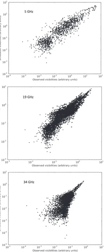
which, at each observed ATCA frequency, allowed us to generate the corresponding visibilities for the IRAC 8μm data set by taking into account the specific configuration of the interferometer. In particular, in order to obtain a perfect correspondence between observed and simulated uv-plane coverage, we used the combined sm.predict and sm. openfromms functions. As described in Section2, the ATCA 5 GHz data set consists of a single pointing. In this case, to perform the simulation, a correction for the ATCA primary beam(∼570″) was applied by multiplying the IRAC 8 μm data with a Guassian profile, centered at the pointing phase center. On the contrary, the ATCA 19 and 34 GHz maps were obtained with a mosaic observing strategy. Therefore, a simulation was performed for each pointing and the correction for the primary beam was applied using a Gaussian mask of 150″ and 80″, respectively. Figure 6 shows the simulated versus observed visibilities at each frequency. In these plots, in order to minimize the correlations in the uv-plane, we binned the u, v cells in 10-minute bins at 5 GHz and 1-minute bins at 19 and 34 GHz, where the difference in bin width reflects the different integration time at the various frequencies. We computed the Pearson correlation coefficient,11ρ, and obtained: ρ8,5= 0.936 ± 0.002, ρ8,19 = 0.848 ± 0.002, ρ8,34 = 0.783 ± 0.009, indicating that the correlation strength slightly weakens as we go from 5 to 19/34 GHz. Note that the correlation errors have been computed from the binned data, in linear scale, taking into account the number of data points (N−1/2) and their standard deviation.
The simulated IRAC 8μm visibilities were then imaged to allow verification of the robustness of the IR—radio correlation in real space. To minimize potential biases arising from the imaging process, we re-created the observed ATCA maps by using the same deconvolution parameters as for the simulated data set. In particular, all the observed maps were re-generated using the same Högbom algorithm and the multiscale cleaning method (Cornwell2008), with three windows of 0, 5, and 15
pixels, which we used for the IRAC simulated maps. The pixel size of all maps was set to 1 2, and to each map the primary beam correction was applied. Figure7illustrates, for the case of the ridge, a morphological comparison between the simulated IRAC 8μm and the observed ATCA 5, 19, and 34 GHz data. At 5 GHz(top panel), both the 8 μm and radio continuum emission peak in the southeast part of the ridge, although clear descrepancies can be noticed between the two emission components. Indeed, radio emissionfills a bubble-like structure located to the northeast of the ridge, for which no 8μm emission is detected. Such differences become even more evident at 19 and especially at 34 GHz (middle and bottom panels): while the 8 μm and microwave emission peaks still spatially coincide toward the east side of the ridge, the west side is characterized, in the cm maps, by a prominent shell-like structure and by a spur with no IR counterpart. These shell-like structure and the spur are the same as discussed in Section3.1.
11
The Pearson correlation coefficient provides an indication of the quality of a least squaresfitting to the data. The coefficient can take values from +1 to −1, where+1 indicates a total positive correlation, 0 indicates no correlation, and −1 indicates a total negative correlation.
4.2. Spectral Index Map
Ideally, we should estimate the amount of microwave excess in the ATCA data by extrapolating the low-frequency observations (5 GHz) to the high-frequencies (19 and
Figure 6. Simulated IRAC 8 μm vs. the real ATCA visibilities. At 5 GHz (top panel), we notice a hint of a possibly residual correlation at high values of the visibilities.
Figure 7. Simulated IRAC 8 μm observations (white contours) overlaid on the observed ATCA data. From top to bottom: 5 GHz(750 B configuration), 19 and 34 GHz(EW 352 configuration).
9
34 GHz) and then by comparing the result with the CBI 31 GHz measurement. Since different interferometer con fig-urations correspond to different amounts offlux loss, a correct approach to this problem would entail filtering the data in the uv-plane to assure that, at each frequency, we are sensitive to emission on the same angular scales. However, given the poor overlap in the visibility plane of the ATCA data set, if we followed this strategy we would remain with virtually no data to analyze.
To circumvent this problem, we considered only low frequency data, and in particular, a combination of our new 5 GHz data and of archival ATCA 1.4 GHz data from WU97. These two data sets are characterized by sufficient overlap in the uv-plane to allow the generation of a reliable spectral index map. To this end, the uv- range of the 1.4 GHz data was truncated to match the shortest uv-coverage of the 5 GHz data (e.g., 1.1 kλ). In addition, since the 5 GHz data still have a denser uv-coverage at short spacings, we truncated these to the same maximum uv-distance of the 1.4 GHz data set(e.g., 20.55 kλ), in order to guarantee a similar shape of the weighting function during the imaging process. It is important to emphasize that this operation does not lead to matched beams at 1.4 and 5 GHz, but simply mitigates the influence of extended structures at 1.4 GHz, and avoids underweighting of the short spacings at 5 GHz. After cleaning, the 1.4 and 5 GHz maps were restored with the same synthetic beam (15″). The maps were then converted in Jy pixel−1units, and pixels below three times the standard deviation computed for each map were discarded. Finally, for each pixel the spectral index (Sν∼ να) was computed using the relation:
S S log log 5 1.4 . 6 5 GHz 1.4 GHz
(
)
( ) ( ) a =Figure 8 shows the spectral index map, and its associated uncertainty map, obtained following the aforementioned steps. The noisy behavior, especially at the edges of the central stucture (the ridge) and of the two shells, likely derives from small differences of the synthetic beams at 1.4 and 5 GHz. Note that emission contribution on specific spatial scales might differ
from pixel to pixel, introducing a bias on the reconsctructed spectral index map that is difficult to quantify.
Although we cannot directly estimate the uncertainty associated with the interpolation of the sampling function, it is commonly accepted that this is a function of the uv-weigths, hence of the noise. Therefore we assume that the error map obtained by considering the average rms is a good representa-tion of the uncertainty of the spectral index map. In particular, we determined the error map in each pixel by propagating Equation(4), i.e., as:
S S 5 GHz 5 GHz 1.4 GHz 1.4 GHz log 5 1.4 , 7 2 2 ( ) ( ) ( ) ( ) ( ) a s s D = + ⎜ ⎟ ⎛ ⎝ ⎜ ⎞ ⎠ ⎟ ⎛ ⎝ ⎜ ⎞ ⎠ ⎟ ⎛ ⎝ ⎞ ⎠
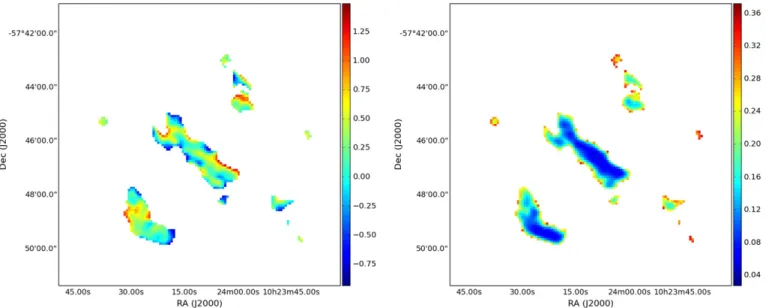
whereσ was evaluated at different positions of the maps and then averaged. We emphasize that the above relation does not take into account modeling errors and/or systematics, which are difficult to quantify. As shown in Figure8, right panel, the uncertainty in the central part of the ridge and in a large part of the southern shell varies between+0.05 and +0.1, while at the edges of the emission regions it increases up to about+0.3.
If we exclude the noisy pixels(i.e., those with an associated uncertainty greater than 0.1), the mean of the spectral index distribution is+0.20 ± +0.22. This is consistent (within 1.5σ) with optically thin free–free emission (α = −0.1), likely due to the ionizing flux from the OB stars in the Wd2 cluster. However, the dispersion around the mean is quite significant. In particular, both the ridge and the west shell are characterized by positive spectral indices. Benaglia et al. (2013) have
recently published two spectral index maps of RCW 49: the first one, derived from the combination of archival ATCA 1.4 and 2.4 GHz data,12covers both the ridge and the shells, while the second, generated from newly obtained 5.5 and 9.0 GHz data, covers only the ridge. The 1.4–2.4 GHz spectral index map is sensitive to angular scales up to several arcmins. The
Figure 8. Left: spectral index map obtained by combining the 5 GHz new observations of the core of RCW 49 with ATCA archival data at 1.4 GHz. The Sν∼ να
convention is used. Right: spectral index error map.
12
5.5–9.0 GHz map is sensitive only up to scales of the order of 100″, that is a smaller scale than the maximum one that our 1.4–5.0 GHz map is sensitive to (∼3 4). The spectral index map obtained from the lower frequency data (their Figure 5)
appears to be fully compatible with optically thin free–free emission. This map also shows a possible contribution from synchrotron emission, especially along the northern side of the ridge and in the west shell. Conversely, the spectral index map associated with the higher frequency data (their Figure 6)
shows positive spectral indices. Indeed a large fraction of the ridge appears to be characterized by spectral indices greater than+0.3, in agreement with our analysis. Interestingly, values of the order of+0.6 are typically associated with stellar winds (e.g., Panagia & Felli 1975) and in general, a global
distribution with rising spectral indices might corroborate the hypothesis, advanced byWU97, that the ridge is the product of the direct collision between the high-velocity winds produced by WR20a and WR20b in the two shells or alternatively, of a collision between the two shells before merging. Remarkably, this collision scenario could also explain the increase of dust temperature along the ridge noted by the same authors.
4.3. No Evidence for Self-absorbed Free–Free Emission As we discussed in Section2, one of the main objectives of the ATCA observations was to assess the presence, in the core of RCW 49, of compact high-density components that could account for an inverted emission spectrum at microwave frequencies. In the Altenhoff et al. (1960) approximation, the
free–free optical thickness, τff, is a function of Te,ν and EM according to: T 0.08235 EM, 8 ff e 1.35 GHz 2.1 ( ) t - n
-where Teis in K,ν in GHz and EM in pc cm−6. For Teof the order of 8000 K, we expect τff > 1 at 31 GHz, which is the frequency of the CBI tentative detection of AME in RCW 49, when EM is greater than∼109pc cm−6. These extremely high emission measures are typical of hyper-compact HII regions
(HCHII), which are also characterized by high electron
densities (ne > 106cm−3) and linear diameters of less than ∼0.05 pc. The very small size of these objects make them good candidates for being responsible for the emission observed by the CBI while remaining virtually undetected in its low-resolution beam. Moreover, the existence of HCHIIs in the core
of RCW 49 would be consistent with a triggering scenario, which is known to be common in Galactic HII regions
(Elmegreen 1998; Deharveng et al. 2005). It is remarkable,
from this point of view, that the GLIMPSE observations of RCW 49 have indeed allowed the identification of some 300 likely young stellar objects (YSOs), representing a new generation of star formation, possibly triggered by the stellar winds and shocks associated with the Wd2 cluster (Whitney et al. 2004). This YSO population is found in six different
regions spread across RCW 49, none of which coincides with the 31-GHz CBI emission peak. The closest region (denoted region“3” by Whitney et al.2004) is situated to the southwest
of the CBI peak, and at a distance of∼2′.
From the analysis of the H109α data set described in Section 3.2, we estimated the emission measure and electron density at three different positions along the ridge. We recall that no line emission was found, above the sensitivity level, at
any other locations, although we should emphasize that the thermal continuum emission also encompasses only ∼1/20th of the 7 8 × 5 6 covered area (roughly 147 beams out of 2950).
Table4shows that the average EM is∼160 pc cm−6, with a corresponding ne of only ∼13 cm−3. These values are indicative of ionized gas denser than in typical ISM conditions, for which 0.03 < ne < 0.08 cm−3 (Haffner et al. 2009), supporting the compressed-by shocks hypothesis formulated byWU97, yet this same gas appears to be much more diffuse than in HCHIIs. From the non-detection of H109α, we can set
lower limits for the electron temperature and emission measure through most of the 5 GHz map. For this purpose, we assume as representative of the non-detection region, Tc ; 60 mJy beam−1andΔV = 8.2 km s−1. The latter is the average value for the H109α line in regions A, B, and C. Setting the detection threshold at 3σ, where σ = 2.6 mJy beam−1, and using Equations (1)–(4), we obtain Te > 9740 K, EM> 376 pc cm−6, and ne> 19.4 cm−3. Therefore our RRL measurements cannot completely rule out the presence of HCHIIs in the core of RCW 49. However, considering that the
spectral index map derived in Section4.2shows no evidence of self-absorbed free–free emission (α ∼ 2), which would certainly characterize such dense condensations of ionized material, we confidently state that it is unlikely that the CBI detection can be attributed to a hidden population of HCIIs.
5. DISCUSSION
The main limitation to keep in mind in interpreting our results is the fact that the ATCA is an interferometer working at arcsec resolution and as such it is subject to significant flux loss on angular scales larger than a few arcmins. In our case, this means that, although the area imaged with the ATCA is 7 8× 5 6, at 5, 19, and 34 GHz, the emission on angular scales larger than 3 4, 1 7, and 1′, respectively, is filtered out. The total 31 GHz flux detected by CBI toward RCW 49 in a 6 8 beam is 146.5± 5.2 Jy. If we integrate the ATCA 5 GHz flux in a similar aperture, we obtain 10.3 Jy which, when extrapolated to 31 GHz using the mean spectral index value (+0.20 ± +0.22) derived in Section4.2, gives 14.82 Jy, that is ∼10% of the CBI observed flux. A similar calculation at 19 and 34 GHz provides, respectively, 31 GHz projected fluxes of 10.18 Jy and 3.11 Jy corresponding to 7% and 2% of the CBI flux. These estimates clearly show that, because at all ATCA frequencies we are losing an important fraction offlux, we have to be careful in generalizing the results of our analysis, especially those regarding the spectral indices. However, it is still possible that, due to the uncertainties inherent to the filtering process in the uv-plane, more than the 30% of the spectral indices are actually positive and not consistent with the canonical value for optically thin free–free emission. In the hypothesis where this rising can be ascribed to a collission between shells or stellar winds, it is hard to imagine that such an energetic phenomenon would affect the emission only on small angular scales. Alternatively, we can speculate that the rising that we observe between 1.4 and 5 GHz is already indicative of AME at these low frequencies. If this was the case, the implication would be that PAHs with a larger size range than typically adopted by spinning dust models (3.5–100 Å, e.g., Ali-Haïmoud et al. 2009) are likely
contributing to the emission. 11
One important thing to notice is that in RCW 49 the location of the CBI peak is offset(∼50″) with respect to the peak of dust emission(see Figure1). This is also the case of RCW 175, for
which Tibbs et al. (2012) have shown, by means of a detailed
modeling analysis of the dust content of the region, that the AME peak does not coincide with the peak of the PAH and VSG spatial distributions, and that such a shift cannot be attributed to instrumental effects, e.g., the CBI pointing error (up to 30″) or its low angular resolution. This finding alone suggests that either the detected AME is not due to spinning dust, or if the origin of the emission is indeed spinning dust, other factors(such as gas ions, etc.) might play a pivotal role in triggering this type of emission, as discussed in Tibbs et al.(2012).
6. CONCLUSIONS
We presented the analysis of ATCA multi-frequency observations (5, 19, and 34 GHz) of a 7 8 × 5 6 region centered on the core of RCW 49, the brightest HIIregion in the
southern hemisphere. At 5 GHz we observed both the continuum and the H109α hydrogen recombination line. Using this new ATCA data set, we investigated the potential correlation between the radio continuum emission at each observed frequency and the 8μm emission, which is dominated by the 7.7μm feature commonly attributed to PAHs. Our analysis shows that, overall, the correlation persists from short (5 GHz) to long wavelengths (34 GHz), and from large (∼3 4) to small(0 4) angular scales. However, we found an indication of a weakening of the correlation going to higher frequencies and to small angular scales. By combining, respectively, new and archival 5 GHz and 1.4 GHz ATCA data, we generated a spectral index map (and its corresponding error map) for the region, encompassing both the ridge and the shells. The spectral index distribution is globally consistent with optically thin free–free emission, although it is characterized by a large dispersion. In particular,∼30%, 20% and 10% of the spectral indices are greater than +0.3, +0.4 and +0.5, respectively, with an average error of less than+0.1. These positive indices are found mostly along the south side of the ridge and of the west shell. This rising of the spectral index distribution might suggest that other mechanisms, other than spinning dust, are responsible for the microwave excess observed by CBI, such as shocks due to a collision event either between the west and east shells or between the stellar winds generated by WR20b and WR20a, as speculated by WU97. Finally, the combined analysis of the spectral index map with the H109α recombina-tion line, marginally detected at three posirecombina-tions along the ridge, appears to suggest that the core of RCW 49 is likely not harboring very compact sources such as HCHIIregions, thus
not supporting an inverted free–free emission scenario as explanation for the CBI 31 GHz excess.
We believe that this study has mostly shown the importance of obtaining high angular resolution observations even for sources which have been studied for more than a century, like HIIregions. These observations are in fact key in revealing the
complexity of physical mechanisms at work in these objects, in particular in very extended and evolved ones such as RCW 49. Without this detailed information it is difficult to interpret
unambiguously the emission seen at relatively low angular resolution at microwave frequencies.
The authors would like to thank the anonymous referee for his/her constructive comments and Dr. Phil Appleton for useful discussions. C.D. acknowledges support from an STFC Consolidated Grant (ST/L000768/1) and an ERC Starting Grant(no. ∼307209).
REFERENCES
Ali-Haïmoud, Y., Hirata, C. M., & Dickinson, C. 2009,MNRAS,395, 1055
Altenhoff, W., Mezger, P. G., Wendker, H., et al. 1960, Veröff Sternwärte Bonn, 59, 48
Battistelli, E. S., Carretti, E., Cruciani, A., et al. 2015,ApJ,801, 111
Benaglia, P., Koribalski, B., Peri, C. S., et al. 2013,A&A,559, 31
Benjamin, R. A., Churchwell, E., Babler, B. L., et al. 2003,PASP,115, 953
Brand, J., & Blitz, L. 1993, A&A,275, 67
Caswell, J. L., & Haynes, R. F. 1987, A&A,171, 261
Churchwell, E., Mezger, P. G., & Huchtmeier, W. 1974, A&A,32, 283
Cornwell, T. J. 2008,ISTSP,2, 793
Davies, R. D., Dickinson, C., Banday, A. J., et al. 2006,MNRAS,370, 1125
Day, G. A., Caswell, J. L., & Cooke, D. J. 1972, AuJPA,25, 1
Deharveng, L., Zavagno, A., & Caplan, J. 2005,A&A,433, 565
Dickinson, C. 2013,AdAst,2013, 4
Dickinson, C., Casassus, S., Pineda, J. L., et al. 2006,ApJ,643, 111
Dickinson, C., Davies, R. D., Allison, J. R., et al. 2009,ApJ,690, 1585
Dickinson, C., Davies, R. D., Bronfman, L., et al. 2007,MNRAS,379, 297
Draine, B. T. 2011,ApJ,732, 100
Draine, B. T., & Lazarian, A. 1998,ApJ,508, 157
Elmegreen, B. G. 1998, in ASP Conf. Ser. 148, Origins, ed. C. E. Woodward, J. M. Shull & H. A. Tronson(San Francisco, CA: ASP),150
Everett, J. E., & Churchwell, E. 2010,ApJ,713, 592
Finkbeiner, D. P., Schlegel, D. J., Frank, C., & Heiles, C. 2002,ApJ,566, 898
Furukawa, N., Dawson, J. R., Ohama, A., et al. 2009,ApJ,696, 115
Haffner, L. M., Dettmar, R., Beckman, J. E., et al. 2009,RvMP,81, 969
Inoue, A. K. 2002,ApJ,570, 688
McGee, R. X., & Newton, L. M. 1981, MNRAS,196, 889
McGee, R. X., Newton, L. M., & Batchelor, R. A. 1975, AuJPh,28, 185
Padin, S., Cartwright, J. K., Mason, B. S., et al. 2002,ApJ, 549, 1 Paladini, R., Burigana, C., Davies, R., et al. 2003,A&A,397, 213
Paladini, R., Umana, G., Veneziani, M., et al. 2012,ApJ,760, 149
Panagia, N., & Felli, M. 1975, A&A,39, 1
Piatti, A. E., Bica, E., & Claria, J. J. 1998, A&AS, 423, 127
Pilbratt, G. L., Riedinger, J. R., Passvogel, T., et al. 2010,A&A,518, 1
Planck Collaboration Int. XV 2014,A&A,564, 45
Planck Collaboration XX 2011,A&A,536, 20
Rauw, G., Crowther, P. A., De Becker, M., et al. 2005,A&A,432, 985
Rauw, G., Manfroid, J., Gosset, E., et al. 2007,A&A,463, 981
Sault, R. J., Teuben, P. J., & Wright, M. C. H. 1995, in ASP Conf. Ser. 77, Astronomical Data Analysis Software and Systems IV, ed. R. Shaw, H. E. Payne & J. J. E. Hayes(San Francisco, CA: ASP),433
Scaife, A. M. M., Green, D. A., Battye, R. A., et al. 2007,MNRAS,377, 69
Scaife, A. M. M., Hurley-Walker, N., Davies, M. L., et al. 2008,MNRAS,
385, 809
Shaver, P. A., & Goss, W. M. 1970a, AuJPA,14, 77
Shaver, P. A., & Goss, W. M. 1970b, AuJPA,14, 133
Shaver, P. A., McGee, R. X., Newton, L. M., et al. 1983,MNRAS,204, 53
Tibbs, C. T., Paladini, R., Compiegne, M., et al. 2012,ApJ,754, 94
Todorovic, M., Davies, R. D., Dickinson, et al. 2010,MNRAS,406, 1629
Vacca, W. D., Garmany, C. D., & Shull, J. M. 1996,ApJ,460, 914
van der Hucht, K. A. 2001,NewAR,45, 135
Westerlund, B. 1960, ArA,2, 419
Whiteoak, J. B. Z., Large, M. I., Cram, L. E., & Piestryzynski, B. 1989, PASAu,8, 176
Whiteoak, J. B. Z., & Uchida, K. I. 1997, A&A,317, 563
Whitney, B. A., Indebetouw, R., & Babler, B. L. 2004,ApJS,154, 315