Introducing communication and networking technologies into lab-on-chip systems

DIPARTIMENTO DIINGEGNERIAELETTRICA, ELETTRONICA ED

INFORMATICA

DOTTORATO DI RICERCA ININGEGNERIAINFORMATICA E DELLE

TELECOMUNICAZIONI

XXVI CICLO

INTRODUCING COMMUNICATION AND NETWORKING TECHNOLOGIES INTO LAB-ON-CHIP SYSTEMS

ING. ELENA DELEO

Coordinatore

Chiar.ma Prof. V. CARCHIOLO

Tutor

CONTENTS

1 Introduction 1

1.1 Microfluidics . . . 3 1.2 Motivation and basic idea . . . 5 1.3 Contributions . . . 6 2 Microfluidic technologies: theory, research tools and state of the

art 9

2.1 Introduction to hydrodynamic microfluidics for non physicists 10 2.2 Droplet generation and manipulation . . . 12 2.3 Microfluidic computing and communications . . . 16 2.4 Computational fluid dynamics and simulation tools . . . 18

3 NLoC concept and architecture 21

3.1 Concept and notation . . . 22 3.2 NLoC functions . . . 25 3.3 System architecture . . . 26

4 Information representation 31

4.1 Approaches . . . 31 4.2 Channel capacity . . . 35 4.3 Channel characterization . . . 44

4.3.1 Characterization of distance between consecutive droplets . . . 47 5 Switching droplets in Hydrodynamically Controlled Networks 53 5.1 Controlling the header droplet . . . 56 5.2 Controlling the payload droplet . . . 59 5.3 Further design guidelines . . . 62

6 Experimentation 65

7 Validation through simulation 71

LIST OF FIGURES

1.1 A microfluidic microreactor (reproduced from [1]). . . 2 2.1 Droplets motion in a bi-phase flow: a) first droplet arrival b)

second droplet arrival c) second droplet transition. . . 10 2.2 Microfluidic device generating droplets by means of a coaxial

geometry (reproduced from [2]). . . 13 2.3 Microfluidic device generating droplets by means of a

T-junction geometry (reproduced from [3]). . . 13 2.4 Microfluidics device generating droplets by means of a

flow-focusing mechanism (reproduced from [3]). . . 14 2.5 Fusion of two droplets forced by a laser beam (reproduced

from [4]). . . 15 3.1 A simple microfluidic device, made of a) a component which

generates droplet; b) a sequence of narrow spires in which droplets are mixed; c)a sequence of wider spires, to introduce a delay which allows reactions happen . . . 23

3.2 Possible NLoC system architectures a) Grid topology, b) Ring topology. . . 27 (a) . . . 27 (b) . . . 27 3.3 Droplet encoding a) Presence/absence of droplets b) Distance

between droplets c) Size of droplets d) Substance composing droplets. . . 29 4.1 Droplet encoding a) Presence/absence of droplets b) Distance

between droplets. . . 37 4.2 Setup for the simulation of the T-Junction. . . 38 4.3 Variance of the error σ_E2divided by the square of the droplets

velocity v2at different boundaries of the T-junction assuming ηr = 3.441. . . 39

4.4 CDDas a function of the variance of the noise, σ_E2, for different

values of ∆ when v = 2mm/s. . . 43 4.5 Probability density functions of time interval between

succes-sive droplets evaluated at boundary 10 for several values of ηr

(in decreasing order). . . 45 4.6 Variance of the error σ_E2divided by the square of the droplets

velocity v2at different boundaries of the T-junction assuming ηr = 3.441. . . 48

4.7 Cumulative distribution function FE(e) of the error E and its

Gaussian approximation assuming ηr= 3.441. . . 48

4.8 Values of ∆/v vs. the ratio ηr. . . 49

4.9 Values of σE/v vs. the ratio ηr. . . 49

4.10 Values of the ratio ∆/σE vs. the ratio between the viscosity

List of Figures v

4.11 Values of the ratio ∆/σE vs. the flowrate of the continuous

phase for two different values of the distance from the

njec-tion point. . . 50

4.12 Values of the ratio ∆/σE vs. the distance from the injection point. . . 50

5.1 Distance-based switching. . . 55

5.2 Equivalent microfluidic and electrical circuits for the MNI represented in Figure 5.1. . . 56

(a) Microfluidic equivalent circuit of the MNI . . . 56

(b) Electrical equivalent circuit of the MNI . . . 56

6.1 Prototype of the HCN addressing device. . . 66

6.2 Experimental results for the case when the payload droplet enters Pipe 1. . . 68

(a) Before the header droplet arrives at B. . . 68

(b) After the payload droplet leaves B. . . 68

6.3 Experimental results for the case when the payload droplet enters Pipe 2. . . 69

(a) Condition before the header droplet arrives at B. . . 69

(b) Condition after the payload droplet leaves B. . . 69

7.1 Configuration considered for simulations. . . 72

7.2 Zoomed view of the connection between the bypass channel and the rest of the circuit. . . 72

7.3 Simulation results for the case in which the payload droplet is addressed to the i-th element E_i(Σ). . . 76

(a) Condition before the header droplet arrives at B. . . 76

7.4 Simulation results for the case in which the payload droplet is addressed to the (i + 1)-th element E_i+1(Σ). . . 77 (a) Condition before the payload droplet arrives at the

point B of the i-th MNI. . . 77 (b) Condition after the payload droplet leaves the point B

of the i-th MNI. . . 77 (c) Condition after the payload droplet leaves the point B

LIST OF TABLES

7.1 Parameters characterizing the geometry illustrated in Figure 7.1. . . 73

ABSTRACT

Microfluidics is a science and a technology which deals with manipulation and control of small volumes of fluids flowing in channels of micro-scale size. It is currently used for Labs-On-a-Chip (LoCs) applications mainly. In this context, recently fluids have been used in the discrete form of droplets or bubbles dispersed into another immiscible fluid. In this case, droplets or bub-bles can be exploited as a means to transport digital information between mi-crofluidic components, with sequences of particles (i.e. droplets or bubbles) representing sequences of binary values. LoCs are today realized through monolithic devices in which samples are processed by passing them through a predetermined sequence of elements connected by fixed and preconfigured microfluidic channels. To increase reusability of LoCs, effectiveness and flex-ibility, networking functionalities can be introduced so that the sequence of elements involved in the processing can be dynamically selected. Accord-ingly, in this thesis we introduce the Networked LoC (NLoC) paradigm that brings networking concepts and solutions in microfluidic systems such as LoCs. More specifically, in this paper the need for the introduction of the NLoC paradigm is motivated, its required functions are identified, a system architecture is proposed, and the related physical level design aspects, such as

channel characterization, information representation and information capacity are investigated; finally a switching device is proposed and studied.

CHAPTER

ONE

INTRODUCTION

In the recent years the use of on-chip technologies for chemical and biomedi-cal environments has increased significantly: it is usually referred to as Labs-on-a-Chip(LoC) technology, meaning that different laboratory functions are executed on a single chip, usually fabricated with or various polymers such as polydimethylsiloxane (PDMS) and polycarbonate or glass, plastic, silicon and small in size (from few mm2 to cm2). Such technology allows LoCs to perform extremely complex operations in devices of small size. As an exam-ple of a LoC component, in Figure 1.1 a scheme of an on-chip microreactor is shown [1]; a microreactor is a small size chip in which several substances (the reagents) are injected and then processed in order to perform a desired chem-ical reaction; the labels A1, A2 and A3 in Figure 1.1 show the inlets through which reagents are introduced in the device. After having been injected in the circuit, such reagents move along a tortuous path: this movement mixes them, thus resulting in a chemical reaction. LoCs can be used in several contexts, they require small amounts of reagents, in the order of few µl to pl, and their

Figure 1.1: A microfluidic microreactor (reproduced from [1]).

cost is low. Regardless of such advantages, their place in the market is still quite limited, mainly due to their lack of flexibility [5] [6].

We argue that an increase in flexibility can be achieved by introducing some basic networking functionalities in LoCs systems.

Before moving on to the next sections, let us take a step back and give a brief overview of microfluidics, the branch of physics on which LoC technologies rely.

1.1. Microfluidics 3

1.1

Microfluidics

Microfluidics is both a science and a technology [7] that deals with the control of small amounts of fluids flowing through micro-channels, with sizes in the order of µm. At such scale, systems exhibit the following features:

• Small size: Microfluidic systems have small size and deal with very small samples. This is in contrast with current chemical analysis/syn-thesis that is often realized over large samples.

• Reversibility and, to some extent, predictability: At macro-scale, flu-ids move in a turbulent way. At micro-scale the flow is laminar due to inertia and pressure. If such fluids are incompressible (i.e. their densi-ties do not vary with time and space), then the system is reversible and controllable.

Applications of microfluidics span over a wide range of domains going from inkjet printheads to DNA chips, from micro-propulsion to micro-thermal tech-nologies.

We are interested in droplets microfluidics which is related to the control of the motion dynamics of droplets into microchannels1. In this scenarios, droplets are dispersed into another fluid, which is immiscible with them. This kind of mixtures are generically named dispersions and droplets are techni-cally called dispersed phase, while the immiscible substance, in which they are immersed, is called continuous phase. Current microfluidic technologies allow control of shape, motion and size of particles dispersed in a continuous phase.

1_{In the following we will usually refer to droplets; however, the same can be applied if} the emulsion is in gaseous state, i.e., in the form of bubbles.

Droplet microfluidics can be applied to biological as well as chemical analysis and synthesis. Indeed, it is straightforward thinking to microfluidic systems as an effective tool to transport samples (for instance by means of droplets), in order to make them interact with appropriate substances in highly controlled conditions, and to realize tasks that are common in chemical anal-ysis, with high resolution, sensitivity and precision. In other words droplet microfluidics can be seen as the basic building block of labs-on-a-chip. Re-cently several approaches have been proposed to control the movements of droplets into microfluidic systems. Examples include pure hydrodynamic ma-nipulation (HM), electrohydrodynamic mama-nipulation (EM), thermocapillary manipulation (TM), magnetic manipulation (MM) and acoustic manipulation (AM), based on the following physical principles:

• in hydrodynamic manipulation, geometries of the channels and hydro-dynamic forces are used to move droplets along a sequence of channels; • by electrohydrodynamic manipulation, conductive droplets are driven

along desired paths by appropriately acting on a grid of electrodes; • in magnetic manipulation, droplets containing magnetic beads are

driven by a magnetic field;

• in thermocapillary manipulation, droplets are driven by a temperature gradient, exploiting the – so called – Marangoni effect;

• in acoustic manipulation, acoustic waves are used to modify internal streaming of a fluid.

AM, MM and TM are very sensitive to noise. EM, instead, is still expen-sive and complex. On the contrary, HM is simple to realize and cost effective.

1.2. Motivation and basic idea 5

So, a significant branch of research focuses on this approach. Recents stud-ies have extended the previous preliminary work on HM in microchannels [8] by introducing the innovative concept of ”bubble logic” [9, 10] which con-sists of steering hydrodynamically the flow of droplets into a network of mi-crochannels by means of other properly timed droplets. These aspects will be described in detail in Chapter 2.3.

1.2

Motivation and basic idea

LoCs integrate several microfluidic elements able to perform specific labora-tory functions in a single chip. Such structure allows LoCs to perform ex-tremely complex operations in devices of small size. Currently, LoCs are re-alized as monolithic devices in which samples are processed by passing them through a predefined and ordered sequence of elements.

On the contrary, the cost of LoCs could be reduced, their reusability in-creased and their effectiveness improved by providing more flexibility. In-deed, if LoCs can select the sequence of elements to be involved in the pro-cessing of a given sample in a programmable and adaptive way, then it is possible to use the same LoC system to perform different tasks (even simul-taneously) and to modify the process, if required.

In traditional microfluidic systems this is not feasible because the output of a given element is statically connected by microfluidic channels to the in-put of another element and therefore the sequence of elements that will be tra-versed by any sample is built in the topology of the LoC device. To overcome this limitation, networking technologies can be integrated in LoC systems. We denote the resulting system as Networked Lab-On-a-Chip (NLoC).

1.3

Contributions

It is intuitive that huge research effort is needed to identify and solve the paramount number of open issues involved by the introduction of the NLoC paradigm. In this thesis we address the main networking issues related to microfluidic networking. Indeed, specific contributions of this thesis are the following:

1. We introduce the NLoC concept, identify the required functions and provide the related design guidelines. To this purpose we will provide the basics of microfluidics using a language and a perspective as close as possible to that of the scientists belonging to the computer and com-munications engineering communities. [11] [12] [13]

2. We propose a system architecture that is in line with the design guide-lines mentioned above. [11] [12] [13]

3. We investigate how to represent information in NLoCs. Different ap-proaches are discussed and the most promising are analyzed and com-pared. [11] [12] [13]

4. We provide a preliminary characterization of microfluidic channels in the perspective of information capacity evaluation. [11] [12] [13] 5. We define a solution for a passive microfluidic switch which can be

used to route droplets in the microfluidic network [14] [15] [16] [17] The rest of this thesis is organized as follows. In Chapter 2 a thorough dis-cussion on the basics of droplet microfluidic technologies which are used in the rest of the paper is provided. In Chapter 3 we introduce the NLoC concept,

1.3. Contributions 7

discuss a few architectural options and compare their advantages and disad-vantages. Information capacity and its representation in such environments will be discussed in Chapter 4. In Chapter 5 the Hydrodynamic Controlled Microfluidic Network(HCN) paradigm is proposed, which is based on a pure hydrodynamic microfluidic switching function. In Chapters 7 and 6 simula-tion and prototype experimental results are presented in order to assess the feasibility of the HCN paradigm. Finally, Chapter 8 provides some conclud-ing remarks.

CHAPTER

TWO

MICROFLUIDIC TECHNOLOGIES: THEORY,

RESEARCH TOOLS AND STATE OF THE ART

In this chapter, we provide an overview of the theoretical background required to understand the physical concepts that are at the base of microfluidic com-puting and communications. Such overview is reported in Section 2.1. Then, in Section 2.2 we provide a brief survey of the most relevant techniques for droplet generation and manipulation in the area of microfluidic technologies. In Section 2.3 we report the most relevant results in the area of microfluidic computing and communications. Finally, in Section 2.4 we describe the most popular research tools utilized in microfluidic research.

1 2 A B 1 2 A B 1 2 A B

Figure 2.1: Droplets motion in a bi-phase flow: a) first droplet arrival b) second droplet arrival c) second droplet transition.

2.1

Introduction to hydrodynamic microfluidics

for non physicists

A thorough introduction to droplet microfluidics can be found in [9,18,19]. In the following, we summarize the aspects that are more relevant to our work.

Consider a micro scale cylindrical pipe of length L and diameter of cross-section D where a fluid flows with average velocity v. The flux Q is the volume of fluid traversing any boundary, i.e. cross-section, of the pipe in a unit of time and can be calculated as

Q= vπR2 (2.1)

where R = D/2 is the pipe radius. The value of the flux Q depends on the pressure difference at the ends of the pipe, ∆P. In fact it can be observed that [9]:

∆P

Q ≈

µ L

D4 (2.2)

2.1. Introduction to hydrodynamic microfluidics for non physicists 11

When we consider a channel in which droplets are introduced, the dy-namic nature of the fluid motion inside the pipe changes in a non-linear and history-dependent way: since the dispersed phase and the continuous phase are immiscible, a droplet inside the pipe acts like an obstacle or a plug in the main flow; this introduces an additional resistance to the flow. This additional resistance can be modeled as an additive pressure drop given by

∆PCa≈

σ RCa

2

3 _(2.3)

where σ is the surface tension between the two phases and Ca= µ v

σ (2.4)

is the Capillary number which is a flow dynamic parameter such that a vari-ation of Ca within a given range guarantees to have a good control over the droplet motion. The dependence on the presence of droplets leads the system to have complex dynamics.

Let us consider now a more complex system, where a bi-phase flow moves through a pipe. Then the pipe divides into two branches, which then merge in a new pipe, as shown in Figure 2.1. The lengths of the two branches differ by little percentage, and the pipes have the same section. Accordingly, the pressure drop between A and B is the same for the two pipes, but the hydrody-namic resistance of the shorter branch (i.e. branch 1) is smaller than the one of the longer branch (i.e. branch 2).

Let R1(nd1) and R2(nd2) be the hydraulic resistances of pipes 1 and 2,

respectively, when there are nd1droplets in branch 1 and nd2droplets in branch

2, that is the resistance of pipe i depends on the presence of ndi droplets inside

it.

A droplet arriving at the T-shaped bifurcation in Figure 2.1, denoted as A, will always follow the branch with the smaller resistance: if the shorter

branch is empty, the droplet will certainly flow through this branch because R₁(0) < R2(0). As an example in Figure 2.1a the first droplet (the white one)

goes into the branch 1 because it is empty and it is the path of least resistance. When a second droplet (the black one) arrives at point A, as shown in Figure 2.1b, the resistance of pipe 1 will be R1(1) > R1(0) because the first droplet

already entered branch 1; if R1(1) > R2(0) then the second droplet arriving at

Awill follow branch 2 as shown in Figure 2.1c, thus increasing its resistance to a greater value R2(1).

Of course if the relationship min_{nd1 : R1(nd1) > R2(0)} ≥ 1 holds, then

more than one droplet is necessary in pipe 1 in order to deviate the successive droplet through pipe 2 when it is assumed to be empty. So the path that a droplet travels between A and B depends on the past history of the channel which introduces complex dynamics [20]. This behavior is relevant in droplet microfluidics, because the geometry of bifurcation A as in Figure 2.1 is the most common way to connect pipes in microfluidic circuits.

2.2

Droplet generation and manipulation

Networked Lab-on-a-Chip require high control over motion, size, distance and interaction between small amount of fluids. In droplet microfluidics sev-eral ways to manipulate droplets have been devised [21]. In this section we provide an overview of the techniques that implement droplet generation and manipulation.

A list of common operations performed on droplets is given below: • Generation of droplet: this is the first step of droplet manipulation:

gen-erating droplets of desired size, distance and shape is a basic require-ment of all microfluidic applications and is related to information

cod-2.2. Droplet generation and manipulation 13

Figure 2.2: Microfluidic device generating droplets by means of a coaxial geometry (reproduced from [2]).

Figure 2.3: Microfluidic device generating droplets by means of a T-junction geometry (reproduced from [3]).

Figure 2.4: Microfluidics device generating droplets by means of a flow-focusing mechanism (reproduced from [3]).

ing in the NLoC system. Several devices exist which implement this task [2]. In Figures 2.2, 2.3 and 2.4 such kind of devices are shown. • Fission: droplets can be split to increase system capacity. In fact, each

droplet can be a vessel for various reagents. Accordingly, droplet fis-sion can help to increase system capacity. However, fisfis-sion of one or more droplets into new droplets may be an undesired event in case of presence or distance encoding: in fact this would lead the receiver to misinterpret a sequence of droplets, thus raising an error in the decod-ing process. This can be controlled by choosdecod-ing the substance com-posing the droplets with an appropriate viscosity, to make them remain cohesive.

• Fusion: it is needed in tasks in which the bubbles/droplets work as microreactors, i.e. they transport chemical/biological reagents within themselves and it is critical that they merge when given conditions

oc-2.2. Droplet generation and manipulation 15

Figure 2.5: Fusion of two droplets forced by a laser beam (reproduced from [4]).

cur. So fusion is related to the payload ”processing” in the NLoC envi-ronment. This can be achieved, for instance, by applying to the flow a temperature gradient by means of a laser beam: as shown in Figure 2.5 a laser beam is capable of blocking the interface between the continuous and the dispersed phase; when the second droplet arrives, the interface of the first droplet pushes on the second droplet until they merge and overcome the pressure given by the laser beam. Similarly to the case of fission, also fusion can cause errors in the decoding process. As pre-viously mentioned, this can be avoided by properly choosing the time interval between consecutive droplets.

• Motion: motion of droplets must be controlled and exploited to make droplets flow through programmed paths. This is currently the most challenging aspect of droplet microfluidics and is strongly related to the internetworking capability of the NLoC.

Motion can be implemented by means of various techniques of manipula-tion, other than the hydrodynamic manipulation which is the one we propose to employ in our NLoC case as discussed in Section 1.1.

2.3

Microfluidic computing and communications

Recently the idea to process and transfer information by means of fluid mo-tion has been proposed [22] [8] [23].

As in the context of conventional computing, also in this case hardware de-vices have been designed which perform simple atomic operations. Thus, a microfluidic device is atomic in the hardware. Prakash et al. [22] realized and tested devices which implement some common logical and timing functions: a) a binary AND-OR gate b) a T flip-flop, c) a droplet synchronizer and d)

2.3. Microfluidic computing and communications 17

an oscillator. The AND-OR gate and the T flip-flop are based on an infor-mation encoding mechanism based on presence/absence coding: a droplet in the channel can be identified with a binary value 1 while no droplets in the channel corresponds to binary value 0. Existence of AND-OR and NOT mi-crofluidic functions is a fundamental issue since it is well known that AND, OR and NOT-gates are a functionally complete operator set, so any binary operation can be implemented through a combination of those gates. A flip-flop can be used as a buffer while the oscillator is capable of making a droplet circulate in a circular pipe with a given periodicity. Finally, the synchronizer is a circuit with two inputs and two outputs. Two droplets, each entering from a different entrance with a certain time displacement, are aligned while they traverse the device, so that they exit at the same time.

Also some solutions for encoding/decoding information through microflu-idic circuits have been proposed in [8]. They typically exploit a cascade of two loops like those illustrated in Figure 2.1. There it is evident that the two loops should exhibit the same topology in order to allow reconstruction of the information at the destination. This approach to information encoding is based on tuning the distance between the droplets entering the loop. This can be achieved by appropriately setting the flow rate of the dispersed phase and continuous phase, thus resulting in a range of frequencies at which droplets are generated.

When a train of equally spaced droplets goes through the loop, the complex dynamics described in Section 2.1 arise. As a result the sequence of droplets at the output of the loop is not equally spaced anymore. However a regularity has been observed in them: there is a pattern of distances between consecu-tive droplets that repeats in time, after a certain number of droplets has passed through the loop. It has also been observed that different patterns at the output of the loop are associated with the frequency at which droplets are generated

at the input. In order to reconstruct the initial information, it is necessary that a twin microfluidic loop is used at destination to properly reconstruct the initial distance between droplets, i.e., information is carried in the distance between droplets. Accordingly, these approaches can be also considered for cryptography.

2.4

Computational fluid dynamics and

simula-tion tools

NLoC system design needs for analysis of the droplets’ motion mechanisms in a microfluidic system. To this purpose, several - often integrated - approaches can be considered:

1. Experimentation in microfluidic devices is often the most simple (and accurate) manner to achieve such goal.

2. When experimental study is not possible or too costly, mathemati-cal models can be used. Usually they consist of partial differential equations (PDE). Unfortunately, the resulting system of equations is extremely complex and, in general, it is not possible to find closed form solutions. Alternatively, in order to identify mathematical models, analogies between microfluidic and electrical circuits can be exploited as proposed in [9, 10, 24–26]. In this case, a pressure drop between two different points of a pipe can be identified with a voltage variation; a volumetric flux can be seen as an electrical current and a fluid resis-tance is the analogous of an electrical resisresis-tance.

3. When the analytical solution to the above equations cannot be found, specific software tools can be used. In fact, several software tools exist

2.4. Computational fluid dynamics and simulation tools 19

that numerically solve PDEs, making use of effective and low resource-consuming algorithms.

In the following we focus on such software tools, that have become ef-fective only when powerful computers have been realized. The types of soft-ware that are most commonly used nowadays for microfluidic computation are given below:

• COMSOL [27]: this is a commercial software with a modular struc-ture. Each package is dedicated to a specific physical branch, including microfluidics. It implements several algorithms and solvers which nu-merically solve PDE for a given physical set-up, by means of the Finite Element Method (FEM).

In its simplest configuration, COMSOL has a very intuitive graphical user interface, including i) a simple CAD interface that can be used to describe the geometry and the physics of the investigated system, ii) a tool for setting the options to be used for the numerical solution of the PDE and iii) several tools for pre- and post-processing of the results. The resulting environment provides a user friendly working experience. COMSOL is a software developed from Matlab: as a consequence, a specific package exists which links COMSOL mathematical results (matrices and files) to Matlab. This makes it possible to realize custom postprocessing operations with Matlab.

Major disadvantages are the following: since it is a commercial soft-ware, the number of simulations that can be executed in parallel is lim-ited by the number of available licenses. Moreover, similarly to other multiphysics simulators, it is resource demanding: the parameter which mostly affects its performance is the amount of RAM installed on the machine. For the configurations we studied, the minimum amount of

RAM needed to perform a fifty-minutes simulation, is 8 GigaBytes. • OpenFOAM [28]: this is an open source software developed by the

SGI corporation [29]. It is designed specifically to solve fluid dynamic problems. Like COMSOL, it implements several algorithms to solve PDEs and provides a large number of solvers, suitable for several com-putational fluid dynamic problems. It supports several external pre- and post-processing tools. This makes it very flexible.

Since it is an open source software, the final users can customize the ex-isting packages or create a new one according to their personal needs. The input data describing the geometry and the physical settings of the problem to be solved are given as a text file. On the one hand, this makes it easier to configure a set of configurations to be solved; on the other hand, the absence of a GUI makes the work of the user more complex.

CHAPTER

THREE

NLOC CONCEPT AND ARCHITECTURE

In this chapter we present a framework for Networked Lab-on-Chip (NLoC). More specifically, we will discuss the minimal set of functions that must be implemented by a NLoC and a system architecture that can support them. For each function we will provide alternative approaches that will be analyzed taking into account the design goals listed below:

• Simplicity: Proposed solutions have to be as simple as possible to guar-antee reduced design costs.

• Reliability: Proposed solutions have to guarantee that the receiving NLoC element is able to recover the information sent by the transmit-ting NLoC element with controllable error probability

• Capacity: Proposed solutions have to support information transfer rates acceptable for the typical applications that will exploit NLoC.

• Flexibility: Proposed solutions have to be usable by the largest possible set of NLoC elements regardless of their specific characteristics and application objectives.

• Energy efficiency: Proposed solutions should minimize energy con-sumption in order to guarantee lower heating and – if battery-powered – longer battery duration.

Accordingly, in the rest of this chapter, we will first provide an overview of the NLoC concept and introduce the required notation in Section 3.1. Then, in Section 3.2 we will discuss the functions that are needed in NLoC systems and finally, in Section 3.3 we will propose an architecture which can support such functions.

3.1

Concept and notation

Current microfluidic systems consist of several specialized elements that are able to perform very specific operations, such as detection of a certain element in a sample or chemical operations over molecules. An example of such a system is the device depicted in Figure 3.1, on which a channel composed of three elements is shown: the first one is for the generation of a sample and of a reagent in form of droplets; the second one is a serpentine with very narrow spires for mixing the two droplets; the third part is a larger serpentine, which serves just as an extension of the channel: this is since an evental reaction needs a certain time to occur, before exiting the device. The circles represent the holes by which liquids are injected and expelled into/out from the chip. Typical microfluidic devices can contain tenths of these kind of elements, thus resulting in much more complex design.

3.1. Concept and notation 23

Droplet generation _Delay

Droplet mixing a)

b)

c)

Figure 3.1: A simple microfluidic device, made of a) a component which generates droplet; b) a sequence of narrow spires in which droplets are mixed; c)a sequence of wider spires, to introduce a delay which allows reactions happen

Now, let us consider a microfluidic system Σ that includes a certain num-ber M of elements denoted as E₁(Σ), E₂(Σ), ...., E_M(Σ), respectively. We denote as f (E_i(Σ)) the function performed by E_i(Σ) and as E(Σ)( f ) the element in Σ performing function f . An application, in its simplest form, requires a se-quence of N functions to be performed. Let Φ denote an application and let

f₁(Φ), f₂(Φ), ..., f_N(Φ)represent the sequence of functions it requires.

Accordingly, samples of application Φ must traverse the sequence of elements E(Σ)( f₁(Φ)), E(Σ)( f₂(Φ)), ..., E(Σ)( f_N(Φ)) where the output of an element should be given as input to another element. Currently, transportation from the output of an element to the input of another is performed:

• by manually moving the sample: this of course makes the system much more sensitive to human errors (spreading samples in the laboratory, damaging devices or equipment); moreover it requires time that could be saved by using an automatic control.

• by deploying appropriate dedicated pipes that connect the sequence of elements that will be traversed by the samples: this can significantly increase the complexity into the design of the device; for instance, in some cases it is necessary to develop devices in which channels are connected in three dimensional directions.

We propose to use networking technologies to perform such operation. More specifically, similarly to what is done in the Networks on Chip (NoC) domain [30], we assume that a networking element – that we call microfluidic network interface(MNI) – is attached to each element E_i(Σ) to perform the operations required for efficient, flexible and reliable exchange of samples with the other elements. We call Networked Lab-on-a-Chip (NLoC) the resulting system. Addressing functionality will be needed to make the MNIs communicate as detailed in the next sections.

3.2. NLoC functions 25

3.2

NLoC functions

The objective of this section is to identify and discuss the minimal set of functions required by NLoC assuming that simplicity is the major design goal. We will begin by focusing on the transmission technique that should be employed. Here two approaches are possible: synchronous and asynchronous transmissions. The first approach requires synchronization among all MNIs and this will affect requirements such as simplicity, reliability, energy; for this reason, asynchronous transmission is to be used in the proposed framework. This, however, requires the definition of a data structure, i.e., the packet. In NLoC – such as in traditional networking environments – the packet is divided into a header which contains information needed for performing networking operations and a payload. The header is a sequence of droplets which encodes the required service and/or the address of the element which should provide such service. Instead the payload may be a droplet containing the sample which is the object of the chemical/biomedical process performed by the LoC or a sequence of droplets encoding information exchanged by the elements of the NLoC.

Important issues to be considered are related to addressing and routing. The latter in particular is closely coupled with the logical topology which will be utilized and the type of interactions that the NLoC should support. In the near future it will be more convenient to concentrate the “intelligence” of the NLoC in a single element. Accordingly, the most appropriate model of interaction is of type request/response in which the central intelligence, which we call microfluidic processing unit (MPU) requests to a given element that an operation is performed on a sample. When such operation is completed, the element will respond by sending back the processed sample along with a report on whether the operation was correctly carried out or not. The MPU

according to the programmed job scheduling, will route the received sample to another element requesting the next operation, if any. It follows that the most appropriate logical topology to impose to the NLoC is a star topology. This simplifies the routing in the MNI significantly. In fact, all packets are generated by the MNI and should be delivered to the central hub (i.e. the intelligence).

Another important advantage of using such approach is that it does not require routing to be performed in the MNIs of the NLoC elements. Rout-ing/switching will be performed by the central hub only. These aspects will be clarified in the following.

Finally, note that the above approach simplifies the medium access con-trol (MAC) which might exploit a polling strategy. Polling however has low efficiency and therefore, we believe that in the future more efficient MAC schemes should be considered.

3.3

System architecture

In this section we will identify an architectural approach which fits with the design guidelines identified in the previous section. Starting from the logical star topology introduced in the previous section, as far as we want to maintain the capability of the NLoC to exchange droplets among LoC elements, the physical implementation of the star topology requires that the switching facil-ities of the system as a whole are concentrated into an MPU. However, use of an hydrodynamic switching matrix at the MPU would result in a prohibitive complexity and cost. So, alternative solutions should be implemented.

In the NoC literature all networking elements – named routers – have the same functionalities and are connected according to a grid topology [30] as

3.3. System architecture 27

(a) (b)

Figure 3.2: Possible NLoC system architectures a) Grid topology, b) Ring topology.

shown in Figure 3.2a. This is not the most convenient solution for NLoCs, at least not at this time, for the following reasons:

• The grid topology requires each network element to be connected to its four neighbors by two directed channels. Realization of the micro-pumps required to operate all channels may cause a dramatic increase in cost and reduce the possibility of downscaling and integrating all the system.

• Hydrodynamic routers are complex systems and therefore replicating them many times could increase the overall complexity of the NLoC and, thus, again the cost.

where MNIs are connected through a ring. A router R, including also the MPU functionalities discussed in the previous section, is connected to the same ring and it is either the destination of the information generated by the MNIs or the source of all packets directed to the MNIs. Accordingly, the logical topology of the NLoC network is a star – as required in Section 3.2 – even if the physical topology is a ring.

Use of a ring topology allows to maintain the operations run by the MNIs extremely simple. In fact, the MNIs simply need to distinguish packets di-rected to them and forward them accordingly. Furthermore, they must per-form a medium access control (which might be extremely simple and based only on polling operated by the router). Finally, they will have to generate packets which will reach the router R.

Comparing the two types of topology, it can be shown that the overall length of the pipes in the grid case is higher than in the ring case. This impacts the energy efficiency since longer pipes require higher pressure to be applied at the ends of the pipes and, therefore, higher energy costs. In fact, note that in the grid topology case, the overall length of the pipes is approximately

l_{Grid≈ 4m(m − 1)} (3.1)

where we assume that the M NLoC elements are located in a m_{× m grid} (ob-viously M = m2). Instead, in the case of ring topology, it can be demonstrated that the overall pipe length is approximately

l_Ring≈ 

(2m2+ 2m_{− 4) if m is even.}

(2m2+ 4m_{− 6) if m is odd.} (3.2) By comparing the overall pipe lengths given in eqs. (3.1) and (3.2) we note that lGrid> lRing for all significant values of m.

3.3. System architecture 29

Finally, observe that in the architecture shown in Figures 3.2 the router R incorporates the MPU functionalities discussed in the previous sections, i.e. it is the element which is able to perform processing [31] and can be programmedin order to implement the logic of complex applications over the NLoC platform. According to the proposed approach, the router R is the only manager of complex tasks. Again this fits with the guidelines provided in Section 3.2. INFORMATION STRING {00101} v· δTb DISPERSED PHASE DROPLET ENCODER CONTINUOUS PHASE BIT STRING _v· δT_c v· 5δTc {00101} BIT STRING DROPLET

ENCODER DISPERSED_PHASE

CONTINUOUS PHASE ∆Tc {00101} BIT STRING DROPLET ENCODER INFORMATION STRING CONTINUOUS PHASE DISPERSED PHASE ∆Tc {00101} BIT STRING DROPLET

ENCODER DISPERSEDPHASE

CONTINUOUS

PHASE INFORMATIONSTRING

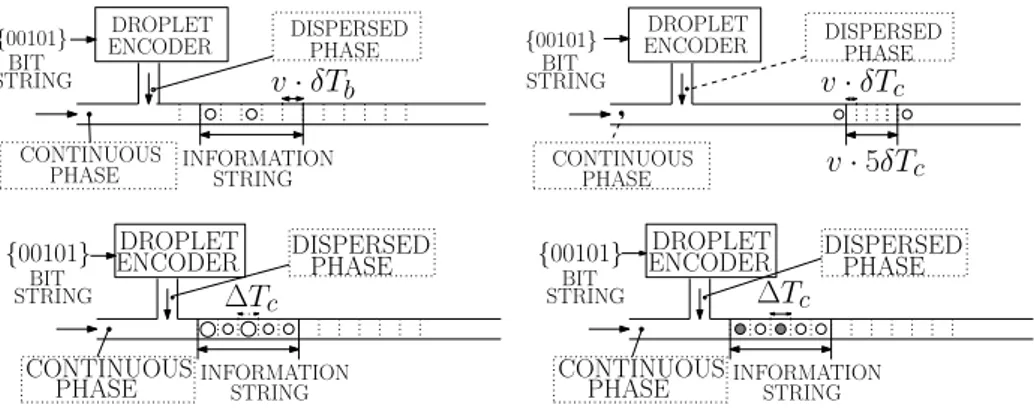
Figure 3.3: Droplet encoding a) Presence/absence of droplets b) Distance between droplets c) Size of droplets d) Substance composing droplets.

CHAPTER

FOUR

INFORMATION REPRESENTATION

In the previous chapters we discussed about the system topology to be con-sidered in an NLoC. However to let the system properly work, we should be able to address the different LoC elements. Accordingly, we need to encode at least the information related to the address of the various elements without disregarding in any case the possibility to encode other information.

So, in this chapter we investigate on the droplet information encoding in microfluidic systems. More specifically, first we will describe different ap-proaches that can be used to represent information. Then, the most promising of such approaches will be analyzed and compared.

4.1

Approaches

It is possible to encode information using different methodologies as dis-cussed in the following:

• Presence/absence of droplets: This is the most obvious way of encod-ing information. Suppose that a strencod-ing of nbbits, {b1, b2, ..., bnb} must

be encoded. Suppose that the string is transmitted at time t0. The

en-coder divides the interval (t0,t0+ nb· ∆Tb) in nb time slots of duration

∆Tbeach and generates a new droplet during the i-th slot if bi= 1, while

does not generate any new droplet if bi= 0. For example, in Figure 4.1a

we show the behavior of the encoder when we assume that the string to be transmitted is_{{00101}. Note that the receiver must implement the} appropriate set of functionalities required to decode the information re-ceived through a train of droplets. If such methodology is employed, errors occur if different droplets belonging to the same train suffer dif-ferent delays in the microfluidic channel and the receiver misinterprets the time slot where a certain droplet is located. Obviously, the larger is ∆Tb, the lower is the probability that errors occur; however, large values

of ∆Tb cause low information rates. The selection of the most

conve-nient value of ∆Tb requires availability of detailed channel models and

knowledge of the interactions between the channel and the operations performed by the receiver. However these models are not available so far and therefore, call for basic research in the area of microfluidic sys-tem characterization and modeling.

• Distance between consecutive droplets: In this case several infor-mation bits are encoded in the distance between consecutive droplets. More specifically the string _{b1, b2, ..., bnb} is mapped to an integer

value X . Then the encoder generates two droplets: one is transmit-ted immediately, the other after a time interval equal to X_{· ∆T}c.1 As an

1_{Observe that as compared to the case when information is coded in the} presence/ab-sence of droplets, in this case ∆Tc< ∆Tbbecause ∆Tbis lowerbounded by the need to avoid

4.1. Approaches 33

example, in Figure 4.1b we show the behavior of the encoder assuming that the string to be transmitted is_{{00101} again, and that the value of} X corresponding to such string is X = 5. Also in this case errors oc-cur if the two droplets are subject to different delay and therefore the receiver achieves a wrong estimation of X . Obviously, in this case the larger is ∆Tc, the lower the probability that estimation of X is erroneous;

however, large values of ∆Tc cause low information rate. Accordingly,

as discussed in case of information encoding based on the presence/ab-sence of droplets, appropriate channel models are required.

• Size of the droplets: In this case coding exploits the capability of gen-erating (and then distinguishing) droplets with different size. As an example, we can consider the case in which droplets can be generated and distinguished based on two different sizes. Small droplets are used to represent ’0’s whereas large droplets are used to represent ’1’s. Such methodology can be considered as a generalization of the “Presence/ab-sence of droplets” methodology (in that case the size of small droplets was zero, i.e., absence of the droplet). In Figure 3.3c, we show the behavior of the encoder when the string to be represented is the usual one, i.e.,_{{00101}. It follows that errors can occur due to the same} rea-soning discussed above. Furthermore, while traversing the microfluidic channel, droplets will be subject to deformations which may also cause errors at the receiver. Obviously the probability of such errors decreases when the difference in the size of the droplets increases.

Finally, note that the information rate can be increased by considering several droplet sizes to encode symbols representing several bits. As an example, we can encode symbols representing two bits by generating

droplets with four different sizes. This increase in the encoding rate is however masked by larger probability of errors because distinguishing between several droplet sizes may be an operation more prone to errors. • Substance composing the droplets: Information is encoded in the sub-stance composing the droplets. Implementation of transmitters which perform such encoding policy is very simple, because different pumps are used, which is a clear advantage. At the receiver, solutions are re-quired which are able to distinguish droplets made of different sub-stances which involves significant complexity. In Figure 3.3d, we show the behavior of the encoder when the string to be represented is again {00101}. In this case errors are caused by wrong processing operations on the droplets at the receiver. Observe that the probability of such errors decreases as the difference in the physical parameters and char-acteristics of the substances utilized to encode bits increases. However, as such difference increases, the behavior of the corresponding droplets in the microfluidic channel becomes much different and sometimes un-predictable.

Accurate regulation of the droplet size at the transmitter or analysis of the substances composing the droplets at the receiver are extremely complex and costly operations with current technologies; so it can be expected that the first generation of NLoCs will employ information encoding schemes based on the presence/absence of droplets or on the distance between consecutive droplets. Furthermore, choice between these two encoding schemes impacts on the design of the microfluidic network devices and, consequently, on the manufacturing process and cost. In fact, presence/absence of droplets en-coding requests a strict droplet synchronization as compared to the distance encoding; so we believe that in the next future the best way to encode

infor-4.2. Channel capacity 35

mation is to use the distance DEncbetween consecutive droplets.

Nevertheless, since microfluidic computing devices have been already de-signed which use the presence/absence of droplets (e.g., [22]), in the follow-ing we will compare their channel capacity with what can be obtained by using droplet distance encoding and characterize the propagation for some physical set-ups.

The transmission capacity for an encoding scheme using the presence/ab-sence of droplets is given by:

C_PA= v/∆ (4.1)

where v is the velocity of the droplets (in m/s) and ∆ is the distance (in m) between two consecutive droplets. It can be shown that in case of distance encoding the capacity CDD can be approximated using the relationship

be-tween the mutual information and the entropy (conditioned or not) [32] as C_DD= v S/2 + ∆log2  S √ 2πeσE  (4.2) where e is the Napier’s constant, σE is the standard deviation of the error and

∆ is again the variable representing distance between consecutive droplets. This is an equation in the parameter S: the latter is the maximum value within which distance between consecutive droplets can be choosen in such a way that they do not interact. Let Smax be the value of S which maximizes eq.

(4.2).

4.2

Channel capacity

The encoding of information in droplet microfluidic systems can be per-formed in different ways. Some possible mechanisms are presence/absence

of droplets, distance between consecutive droplets, size of droplets, substance composing droplets. However, accurate regulation of the droplet size at the transmitter or analysis of the substances composing the droplets at the receiver are extremely complex and costly operations with current technologies. Thus, the first generation of HCNs will likely employ information encoding schemes based either on the presence/absence of droplets or on the distance between consecutive droplets.

To this purpose, in Figure 4.1 we show how a string of bits, for example ”00101”, can be encoded in HCNs. More specifically, in Figure 4.1(a) pres-ence/absence encoding is illustrated: a bit ”1” is encoded into presence of a droplet and a bit “0” is encoded into absence of a droplet. In Figure 4.1(b), instead, the bit string is converted into a number, e.g., the string 00101 = 5, and the droplet encoder generates two droplets which are distant 5δ from each other, where δ represents the granularity supported by the HCN and depends on the noise introduced by the microfluidic channel and the precision of the receiver. Observe that, the choice between these two encoding schemes im-pacts on the design of the microfluidic network devices and, consequently, on the manufacturing process and cost. In fact, encoding based on the pres-ence/absence of droplets requires a strict droplet synchronization as compared to distance encoding; accordingly for worth of simplicity, in this paper we will focus on the case of information encoded in the distance DEnc between

con-secutive droplets. In the rest of this section, we will calculate the maximum information rate, CDD, that can flow through a microfluidic channel. To this

purpose, we will exploit two experimental evidences we have observed in our tests:

1. Experimental evidence 1: droplets interact with each others when their distance is below a given threshold ∆ which depends on a large

4.2. Channel capacity 37

number of physical factors. Such interactions usually result in droplets coalescence (i.e. fusion) which may cause errors. If the distance be-tween droplets is higher than ∆, droplets do not interact with each other [33].

2. Experimental evidence 2: given two consecutive droplets, their dis-tance at the receiver, DDec, is different from their distance at the

transmitter, DEnc. The difference between the above distances, E =

D_{Dec− DEnc}, can be regarded as an additive noise in the proposed sys-tem. In Section 4.3 we will show that E can be modeled as a Gaussian random variable characterized by an average value 0 and a variance σ_E2 (see Figure 4.7). Moreover such noise does not depend on the observed point in the micro-channel as illustrated in Figure 4.6.

Figure 4.1: Droplet encoding a) Presence/absence of droplets b) Distance between droplets.

The maximum information rate, CDD, can be written as:

C_DD = max TS  C_S T_S  , (4.3)

Figure 4.2: Setup for the simulation of the T-Junction.

where CS represents the capacity for each channel use when the average time

interval between two consecutive channel uses is equal to TS. As a

conse-quence of Experimental evidence 1, the average time interval between two channel uses must be larger than ∆/v to avoid coalescence, where v is the av-erage velocity of droplets moving in the microfluidic channel. Accordingly, we write TSas

T_S= ∆ + S

v , (4.4)

where S is a positive value. Therefore, (4.3) can be rewritten as follows C_DD= max

TS

v_·CS

∆ + S. (4.5)

In the following, we will first demonstrate that CScan be calculated as:

C_S= log₂   eS  2πeσ_E2  , (4.6)

4.2. Channel capacity 39

1

1.5

2

2.5

0

1

2

3

x 10

distance from J [mm]

σ

E

2

[s

2

]

Figure 4.3: Variance of the error σ_E2 divided by the square of the droplets velocity v2at different boundaries of the T-junction assuming ηr = 3.441.

where σ_E2is the variance of the noise E as mentioned above. Then, we will use (4.6) to demonstrate that CDD is given by:

C_DD= _ v 2πeσ_E2log 2 e−W ( ∆ √ 2πeσ 2_E ) , (4.7)

where W (_{·) is the Lambert W function and is defined through the inverse} relationship

z= W (z)eW(z). (4.8)

Let us start by proving (4.6). First, note that the average time interval between two channel uses is equal to the average time interval between the generation of two consecutive droplets. This can be calculated as the average distance between two consecutive generated droplets, E_{DEnc}, divided by

the average velocity v. Accordingly, we can calculate T_Sas

TS=

E_{DEnc}

v . (4.9)

To avoid coalescence, the distance between droplets set by the transmitter, DEnc, must be larger than ∆. Accordingly, we write DEncas:

D_Enc= ∆ + X , (4.10)

where X represents a positive random variable with average value equal to S, i.e. ηX = S.

It follows that the capacity CScan be written as a function of the mutual

in-formation between the distance of two consecutive droplets at the transmitter and at the receiver, i.e. I(DDec, DEnc). More specifically, CSis given by [32]:

4.2. Channel capacity 41

aas

C_S = max_fX(x):ηX=SI(D_Dec, D_Enc) =

= max_fX(x):ηX=S[h(D_Dec)_{− h(DDec|DEnc})] = = max_fX(x):ηX=S[h(D_Dec)₋

−h(DEnc+ E|DEnc)] =

= max_fX(x):ηX=S[h(D_Dec)_{− h(E|DEnc})],

(4.11)

where h(_{·) is the differential entropy. By assuming that the noise E is} indepen-dent of the distance between the droplets, it follows that h(E_|DEnc) = h(E).

Furthermore, given that the noise E is Gaussian, its differential entropy is given by

h(E) = log₂(√2πeσE). (4.12)

It follows that (4.11) can be rewritten as C_S= max

fX(x):ηX=S

[h(DDec)]− log2(

√

2πeσE). (4.13)

Given that the error is Gaussian with average value equal to 0, the aver-age value of the distance between two droplets at the transmitter and at the receiver is the same. Moreover, if we suppose that the probability that such distance is lower than ∆ is negligible as in [34], we observe that max_fX(x):ηX=S[h(DDec)] is equal to the entropy of an exponential variable (i.e.

the one which maximizes the differential entropy) with average equal to S, that is max fX(x):ηX=S [h(DDec)] = 1_{− log(1/S)} log(2) = log2(e· S). (4.14) By replacing (4.14) in (4.13) we obtain

C_S = log₂(e_{· S) − log2}(√2πeσE) =

= log₂  e_·S √ 2πeσ2 E  , (4.15)

which proves (4.6).

Eq. (4.6) can be used to demonstrate (4.7). To this purpose, let us plug (4.6) in (4.5). Accordingly, we obtain: C_DD= max S>0 v_{· log2}  eS √ 2πeσ_E2  ∆ + S . (4.16)

In order to find the maximum value required in (4.16) we need to evaluate the derivative of log2  eS √ 2πeσ 2_E 

∆+S with respect to S. Then, we must find the

values of S for which such derivative is equal to 0. Accordingly, we have to calculate the values of S such that

∆ + S− S log  √ eS √ 2πσE  = 0_⇒ S  log  √ eS √ 2πσE  − loge= ∆_⇒ Slog  S √ 2πeσE  = ∆⇒ S √ 2πeσE log  S √ 2πeσE  = _√ ∆ 2πeσE. (4.17) By denoting B =log√ S 2πeσE  it follows that BeB=_√ ∆ 2πeσE . (4.18) Therefore B=  log√ S 2πeσE  = W  ∆ √ 2πeσE  , (4.19)

where W (_{·) is the above mentioned Lamber W function. Accordingly, there} is only one value of S which satisfies (4.17), that is

S∗=√2πeσEeW(∆/( √

4.2. Channel capacity 43 1 2 3 4 5 x 10−10 0 10 20 30 40 σ E 2 [m2] C DD [bits/s] ∆=100 µm ∆=300 µm ∆=600 µm ∆=1000 µm

Figure 4.4: CDD as a function of the variance of the noise, σ_E2, for different

values of ∆ when v = 2mm/s.

It is possible to prove that the second derivative of

log2  eS √ 2πeσ 2_E  ∆+S with respect

to S is lower than 0 when S = S∗. So S∗ is the searched maximum value. Finally, by plugging (4.20) in (4.16) we obtain the expression in (4.7) which concludes our demonstration.

In Figure 4.4 we show the impact of the variance of the noise, σ_E2, and the threshold ∆ on the capacity CDD. As expected,

• an increase in σ_E2 decreases system performance in terms of maximum information rate.

• an increase in ∆, that is the minimum droplets’ distance to avoid coa-lescence, results in a decrease in CDD.

∆ σE > e √ 2πe ln 2 e1/ ln 2 2 = 16.4772 (4.21)

In [12] and [13] we have evaluated the value of the ratio ∆/σE as a

func-tion of several design parameters, such as

• ηr, representing the ratio between the viscosity of the continuous phase

ηc and the viscosity of the dispersed phase ηc, i.e. ηr = ηc/ηd. The

corresponding curve is represented in Figure 4.10. In particular, it has been choosen ηc= 6.71· 10−3Pa· s and ηd∈ [1.95 · 10−3, 6.71· 10−3]

Pa_{· s.}

• QC, that is the flowrate at which the continuous phase is injected into

the pipe. To this purpose we represent two curves in Figure 4.11: one was obtained when the distance from the injection point is d = 0.6 mm and the other when d = 2.7 mm.

4.3

Channel characterization

In this section we characterize the noise statistics in the microfluidic channel relevant to information encoding/decoding for different values of the viscosity of the fluids. To this goal, we have run a large set of simulations aimed at the characterization of how droplets flow in microfluidic channels. We have used the OpenFOAM simulator [28] to investigate the standard microfluidic configuration shown in Figure 4.2 and usually denoted as T-junction.

In this configuration there are two inlets (where fluids enter the system), In₁ and In2, and an outlet O. The continuous phase, that is the fluid which

carries the droplets, enters from inlet In1 while the dispersed phase, i.e., the

fluid which composes the droplets, enters from In2. Sections of all Pipes are

0.1_{×0.05 mm}2in size. We assume that the viscosity of the dispersed phase is 6.71_·10−3Pa_{· sec, whereas the viscosity of the continuous phase can assume} a value in the range [1.75_{· 10}−3, 7.8_{· 10}−3] Pa_{· sec.}

4.3. Channel characterization 45 0 0.05 0.1 0.15 0.2 0 0.010.020.030.040.05 δ [sec] η_r = 0.86026 0 0.05 0.1 0.15 0.2 0 0.010.020.030.040.05 δ [sec] η_r = 1.147 0 0.05 0.1 0.15 0.2 0 0.010.020.030.040.05 δ [sec] η_r = 1.7205 0 0.05 0.1 0.15 0.2 0 0.010.020.030.040.05 δ [sec] η_r = 2.294 0 0.05 0.1 0.15 0.2 0 0.010.020.030.040.05 δ [sec] η_r = 3.1282 0 0.05 0.1 0.15 0.2 0 0.010.020.030.040.05 δ [sec] η_r = 3.441 0 0.05 0.1 0.15 0.2 0 0.010.020.030.040.05 δ [sec] η_r = 3.8234

Figure 4.5: Probability density functions of time interval between successive droplets evaluated at boundary 10 for several values of ηr (in decreasing

The dispersed phase entering from inlet In2 forms droplets at the

inter-section point junction J at a constant rate. These droplets will be transported by the continuous phase throughout the channel to the outlet O. The distance between the point J and the outlet O is equal to 2.7 mm. We considered 19 observation points (called boundaries) equally spaced along the branch J_−O. In our experiments we measured the interarrival time between pairs of consec-utive droplets at such boundaries, for different values of the ratio ηr between

the viscosities of the dispersed and continuous phases.

For example, in Figure 4.5 we show the probability density functions of the interarrival time between consecutive droplets at boundary 10, for dif-ferent values of the ratio ηr between the viscosity of the dispersed and the

continuous phase. In Figure 4.5 we observe that the variance of the droplet inter-arrival time increases as the viscosity of the continuous phase increases and, thus, ηr decreases.

This is because when the viscosities of the two fluids differ, they tend to exhibit resistance in motion which leads to a larger variance in the inter-arrival time between consecutive droplets.

As discussed in Section 4.3, the performance of the encoding scheme de-pends on the values of both ∆ and the variance of the error. As far as ∆ is concerned, this does not depend on the boundary where we observe the flux of droplets. On the contrary, we would expect that the variance increases as the distance between the considered boundary and the intersection point J increases, as in traditional communication systems where the signal quality decreases as it propagates through the channel.

Accordingly, in Figure 4.6 we show the value of the variance of the error E observed at different distances from the intersection J. Variations of the values reported in figure, which has been obtained by considering 100 ob-servations, are due to a large number of factors such as pressure fluctuations

4.3. Channel characterization 47

(which occur especially in the proximity of the junction) and imperfections and roughness in the microfluidic channel (which are modeled in OpenFoam through appropriate setting of simulation parameters). Deep investigation of the above phenomena is the subject of current chemical and physical research, see for example [35, 36], and is beyond the scope of this paper. Here we note however that, surprisingly, the variance does not increase in a noticeable way as the distance from the intersection J increases.

This means that, in microfluidic communication channels, the quality of the signal does not decrease as the distance between the sender and the re-ceiver increases. In Figure 4.7, we represent the cumulative distribution func-tion of the error E measured at the intersecfunc-tion distant 1.4 mm from J. Let us notice that the cumulative distribution function of E, FE(e), obtained in our

simulations fits perfectly the cumulative distribution function of a Gaussian random variable. This is expected given that E derives from the interactions between a huge number of particles.

In Figure 4.8, we show the value of ∆/v vs. the ratio ηr. In this figure we

observe that the value of ∆/v increases as the above ratio ηr increases and,

thus, the information capacity of the encoding scheme is expected to worsen. Finally, in Figure 4.9 we show the value of the standard deviation of the error (i.e. the noise), σE, divided by the velocity v, versus the ratio ηr. When

the ratio ηrincreases, σE/v decreases and therefore, the information capacity

increases.

4.3.1

Characterization of distance between consecutive

droplets

In the next chapter we present an example of design of a reliable pure hydro-dynamic switch able to manage the information about the destination address

1 1.5 2 2.5 0 1 2 3x 10 −7 distance from J [mm] σ E 2 [s 2 ]

Figure 4.6: Variance of the error σ_E2 divided by the square of the droplets velocity v2at different boundaries of the T-junction assuming ηr= 3.441. −2 0 2 x 10−4 0 0.2 0.4 0.6 0.8 1 ∆_E [s] F( ∆ E ) [1] Gaussian approximation Experimental results

Figure 4.7: Cumulative distribution function FE(e) of the

error E and its Gaussian approximation assuming ηr =

4.3. Channel characterization 49 1 1.5 2 2.5 3 3.5 0.01 0.011 0.012 0.013 0.014 η_r [1] ∆ [s]

Figure 4.8: Values of ∆/v vs. the ratio ηr.

1 1.5 2 2.5 3 3.5 0 0.5 1 1.5 2x 10 −3 η_r [1] σ E [s]

0 10 20 30 40 50 60 1 1.5 2 2.5 3 3.5 ∆/σ E [1] η_r [1] 0 10 20 30 40 50 60 1 1.5 2 2.5 3 3.5 ∆/σ E [1] η_r [1] convenience regions border

Figure 4.10: Values of the ratio ∆/σE vs.

the ratio between the viscosity of the con-tinuous and dispersed phases.

0 10 20 30 40 50 60 250 260 270 280 290 300 ∆/σ E [1] Q_C [mm3/s] d = 0.6 mm 0 10 20 30 40 50 60 250 260 270 280 290 300 ∆/σ E [1] Q_C [mm3/s] d = 2.7 mm 0 10 20 30 40 50 60 250 260 270 280 290 300 ∆/σ E [1] Q_C [mm3/s] convenience regions border

Figure 4.11: Values of the ratio ∆/σE vs.

the flowrate of the continuous phase for two different values of the distance from the njection point.

0 10 20 30 40 50 60 1 1.2 1.4 1.6 1.8 2 2.2 2.4 2.6 ∆/σ E [1] d [mm] 0 10 20 30 40 50 60 1 1.2 1.4 1.6 1.8 2 2.2 2.4 2.6 ∆/σ E [1] d [mm] convenience regions border

4.3. Channel characterization 51

encoded as distance between droplets. This switch is the MNI illustrated in Figure 3.2b and its purpose is to forward the droplets containing the samples towards the microfluidic element attached to it or let them continue to flow towards the next MNI in the ring.

In this context, it is useful to statistically characterize the distance between droplets, DDec, at the receiving MNI.

By assumption that the noise E is additive and independent on the dis-tance between droplets at the transmitter2, DEnc, thus we can calculate the

probability density function of DDec, that is, fDDec(x) as given below:

f_DDec(x) = ( f_DEnc⋆ f_E)(x), (4.22)

where fDEnc(x) represents the probability density function of the distance

be-tween the droplets at the transmitter, fE(x) represents the probability density

function of the noise, and ’⋆’ represents the convolution product. By recalling that the noise is Gaussian, thus

fE(t) = 1  2πσ_E2 e− t2 2σ 2_{E (4.23)}

and assuming that DEnc is uniformly distributed in the interval [∆, ∆ + Xmax]

(which guarantees a bound on the transmission delay), i.e.,

f_Enc(t) = 

1/Xmax ∆≤ t ≤ ∆ + Xmax

0 otherwise (4.24)

2_{This assumption is justified by the fact that, by assuming that such droplets distance is} higher than ∆, as stated in experimental evidence1, droplets do not interact with each others.

we obtain f_DDec(x) =  +∞ −∞ f_Enc(t) f_E(_{−t + x)dt =} 1 2_{· X}max· ·  erf x_√− ∆ 2σE  − erf x− ∆ − X√ max 2σE  . (4.25)