Reactive and dynamic local search for Max-Clique, does the complexity pay off?

DEPARTMENT OF INFORMATION AND COMMUNICATION TECHNOLOGY 38050 Povo — Trento (Italy), Via Sommarive 14

http://dit.unitn.it/

REACTIVE AND DYNAMIC LOCAL SEARCH FOR MAX-CLIQUE,

DOES THE COMPLEXITY PAY OFF?

Roberto Battiti and Franco Mascia

April 2006

Reactive and dynamic local search for

Max-Clique, does the complexity pay off?

Roberto Battiti and Franco Mascia

Dept. of Computer Science and Telecommunications

University of Trento, Via Sommarive, 14 - 38050 Povo (Trento) - Italy

e-mail of the corresponding author: mascia@dit.unitn.it

April 2006

Abstract

This paper presents some preliminary results of an ongoing investigation about how different algorithmic building blocks contribute to solving the Maximum Clique problem. In detail, we consider greedy constructions, plateau searches, and more complex schemes based on dynamic penalties and/or prohibitions, in particular the recently proposed technique of Dynamic Local Search and the previously proposed Reactive Local Search. The experimental results consider both the empirical hardness, measured by the iterations needed to reach empirical maxima, and the CPU time per iteration.

1

Reactive search and maximum clique

Reactive Search, see [6] for a recent presentation and [4, 5] for seminal papers, advocates the use of machine learning to automate the parameter tuning process and make it an integral and fully documented part of the algorithm. Learning is performed on-line, and therefore task-dependent and local properties of the configuration space can be used. In this way a single algorithmic framework maintains the flexibility to deal with related problems through an internal feedback loop that considers the previous history of the search, see also [13] for a recent work summarizing the state-of-the-art of self-tuning based on instance characteristics, and [8] for a proposal for learning domain-specific backtracking-based algorithms.

The Maximum Clique problem in graphs (MC for short) is a paradigmatic combinatorial optimization problem with relevant applications [15], including information retrieval, computer vision, and social network analysis. Recent interest includes computational biochemistry, bio-informatics and genomics, see for example [14, 9]. The problem is NP-hard and strong negative results have been shown about its approximability [11], making it an ideal testbed for search heuristics.

LetG = (V, E) be an undirected graph, V = {1, 2, . . . , n} its vertex set, E ⊆ V × V its edge set, and G(S) = (S, E ∩ S × S) the subgraph induced by S, where

S is a subset of V . A graph G = (V, E) is complete if all its vertices are pairwise

adjacent, i.e. ∀i, j ∈ V, (i, j) ∈ E. A clique K is a subset of V such that G(K) is

complete. The Maximum Clique problem asks for a clique of maximum cardinality. A Reactive Local Search (RLS) algorithm for the solution of the Maximum-Clique problem is proposed in [3, 7]. RLS is based on local search complemented by a feedback (history-sensitive) scheme to determine the amount of diversification. The reaction acts on the single parameter that decides the temporary prohibition of selected moves in the neighborhood. The performance obtained in computational tests appears to be significantly better with respect to all algorithms tested at the the second DIMACS implementation challenge.

Recently, the authors of [16] proposed a stochastic local search algorithm (DLS-MC), based on a clique expansion phase followed by plateau search after a maximal clique is encountered. Diversification is based on vertex penalties which are dynamically adjusted during the search and on a strict prohibition mechanism to avoid the same vertex being moved multiple times during a plateau search. The DLS-MC scheme is actually a slight simplification of the Deep Adaptive Greedy Search of [10]: vertex penalties are used throughout the entire search, a ”forgetting” mechanism decreasing the penalties is added, and vertex degrees are not considered in the selection. The authors report a very good performance on the DIMACS instances. While the number of iterations (additions or deletions of nodes to the current clique) is in some cases larger than that of competing techniques, the small complexity of each iteration when the algorithm is realized through efficient supporting data structures leads to smaller overall CPU times.

The initial motivation of this work is threefold. First, we want to investigate how the different algorithmic building blocks contribute to effectively solving max-clique instances corresponding to random graphs with different statistical properties. In particular, the investigation considers the effects of using the vertex degree information during the search, starting from simple to more complex techniques.

Second, we want to assess how different implementations affect CPU times. For example, it may be the case that larger CPU times are caused by using a high-level language implementation w.r.t. low-level ”pointer arithmetic”. Having available the original software simplified the starting point for this analysis.

Third, the DIMACS benchmark set (developed in 1992) has been around for more than a decade and there is a growing risk that the desire to get better and better results on the same benchmark will bias the search of algorithms in an unnatural way. We therefore decide to concentrate the experimental part on two classes of random graphs, chosen to assess the effect of degree variability on the effectiveness of different techniques.

Because of lack of space, we present in this paper preliminary results of a larger ongoing investigation.

2

Algorithmic building blocks of increasing complexity

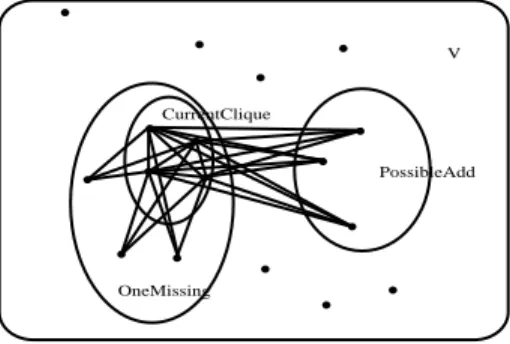
In the local search algorithms, the basic moves consist of the addition to or removal of single nodes from the current clique (a swap of nodes can be trivially decomposed into two separate moves). Two sets are involved in the execution of basic moves: the set

of the improving neighbors POSSIBLEADDwhich contains nodes connected to all the elements of the clique, and the set of the level neighbors ONEMISSINGcontaining the nodes connected to all but one element of the clique, see Fig. 1. Let’s fix the notation. The various simple building blocks considered, are named following the BasicScheme - CandidateSelection structure. The BasicScheme describes how the greedy expansion and plateau search strategies are combined, possibly with prohibitions or penalties. The CandidateSelection specifies whether the vertex degree information is used during the selection of the next candidate move. If it is used, there are two possibilities: of using the static node degree inG or the dynamic degree in the subgraph induced by the

POSSIBLEADDset.

V

OneMissing

PossibleAdd CurrentClique

Figure 1: Neighborhood of current clique.

2.1

Exp-Rand

This basic algorithm is the starting point for all the successive modifications and improvements, see Fig. 2 for the pseudo-code. It searches for the maximum clique in the graph by means of repeated greedy constructions (also called expansions), selecting from

POSSIBLEADDa node at random and restarting from a random node when no expansion

is possible anymore.

1. EXP-RAND(maxIterations) 2. iterations ← 0

3. whileiterations < maxIterations do

4. C ← random v ∈ V 5. EXPAND(C) 6. EXPAND(C) 7. while POSSIBLEADD6= ∅ do 8. C ← C ∪ random v ∈ POSSIBLEADD 9. iterations ← iterations + 1

2.2

Exp-StatDegree

Instead of choosing a random element from POSSIBLEADD, a random node is chosen among the candidates having the highest degree in G. TheEXPAND sub-routine in Fig 2 is modified by substituting line 8 with:

C ← C ∪ { random v ∈ POSSIBLEADDsuch thatdegG(v) is maximum}.

2.3

Exp-DynDegree

In this version, the selection of the candidate is not based on the degree of the nodes in

G, but on the degree in POSSIBLEADD. Line 8 becomes:

C ← C ∪ { random v ∈ POSSIBLEADDsuch that_{degPOSSIBLEADD}(v) is maximum}.

2.4

ExpPlat-Rand

This algorithm alternates between a greedy expansion and a plateau phase, choosing between the possible candidate nodes at random.

During the expansion phase, new vertices are chosen randomly from POSSIBLEADD

and moved to the current clique. When POSSIBLEADD is empty and therefore no further expansion is possible, the plateau phase starts. In this phase, a node belonging to the level neighborhood ONEMISSINGis swapped with the only node not connected to it in the current clique. The plateau phase does not increment the size of the current clique and it terminates as soon as there is at least an element in the POSSIBLEADD

set, or if no candidates are available in ONEMISSING. As it is done in [16], nodes cannot be selected twice in the same plateau phase. In order to avoid infinite loops, the number of plateau searches is limited to maxPlateauSteps.

Starting from EXP-RAND, the base algorithm is adapted to deal with the alternation

of the two phases, see Fig. 3. Let us note that, ifPLATEAUreturns with POSSIBLEADD6= ∅

then a new expansion is tried as described in line 5-7. The iterations are incremented by 2 during a swap because it is counted as a deletion followed by an addition.

2.5

ExpPlat-StatDegree

This algorithm alternates between an expansion and a plateau phase, choosing the possible candidate having the highest degree. The restart is done after starting from a random node. This algorithm is a modified version of EXPPLAT-RAND(Fig. 3) with the static degree selection of EXP-STATDEGREE.

2.6

ExpPlat-DynDegree

This algorithm is the same of EXP-DYNDEGREE, having a plateau phase.

The dynamic degree heuristic affects only the selection of the next candidate for the expansion phase, while in the plateau phase the selection of nodes is based on the static degree.

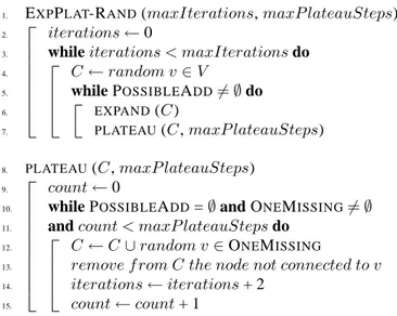
1. EXPPLAT-RAND(maxIterations, maxP lateauSteps) 2. iterations ← 0

3. whileiterations < maxIterations do

4. C ← random v ∈ V

5. while POSSIBLEADD6= ∅ do

6. EXPAND(C)

7. PLATEAU(C, maxP lateauSteps)

8. PLATEAU(C, maxP lateauSteps)

9. count ← 0

10. while POSSIBLEADD=∅ and ONEMISSING6= ∅

11. andcount < maxP lateauSteps do 12. C ← C ∪ random v ∈ ONEMISSING

13. remove f rom C the node not connected to v 14. iterations ← iterations + 2

15. count ← count + 1

Figure 3: EXPPLAT-RAND algorithm, alternating between EXPAND and PLATEAU

phases.

2.7

DLS-MC

This is the algorithm proposed in [16]. To achieve diversification during the search, penalties are assigned to vertices of the graph and they influence the selection of nodes. The algorithm alternates between expansion and plateau phases. Selection is done by choosing the best candidate among the set of the nodes in the neighborhood having minimum penalty.

When the algorithm starts, the penalty value of every node is initialized to 0 and when no further expansion or plateau moves are possible, the penalties of nodes belonging to the clique are incremented by one. All penalties are decremented by one afterpd

(penalty delay) restarts, see the cited paper for additional details and results.

2.8

ExpPlatProhibition-Rand

This algorithm is the same algorithm of EXPPLAT-RAND, but it also uses prohibitions. Every time a node is added or removed from current clique, it is prohibited for the next

T iterations. Prohibited nodes cannot be considered among the candidates of expansion

and plateau phases. When all the moves are prohibited a restart is performed.

2.9

RLS

RLS [7] alternates between expansion and plateau phases, like DLS-MC, but it selects the nodes among the non-prohibited ones which have the highest degree in POSSIBLEADD. The prohibition time is adjusted reactively depending on the search history. Restarts

are executed only when the algorithm cannot improve the current configuration within a fixed number of iterations, see the paper for details.

2.10

RLS-StatDegree

This algorithm is a modification of RLS which uses the static degree instead of the dynamic degree selection.

3

Computational experiments

Performance and scalability tests are made on two different classes of random graphs:

Binomial random graphs A binomial graphGIL(n, p), belonging to Gilbert’s model

G(n, p) is constructed by starting from n nodes and adding up ton(n−1)₂ undirected edges, independently with probability0 < p < 1. See [2] for generation details.

Preferential Attachment Model A graph instanceP AT (n, d), of the preferential attachment

model, introduced in [1] is built by starting from a single node and adding successively the remaining nodes. The edges of the the newly added nodes are connected to d existing nodes, with preferential attachment to nodes having a

higher degree, i.e. with probability proportional to the number of edges present between the existing nodes.

In binomial graphs, the degree distribution for the different nodes will be peaked on the average value, while in the preferential attachment model, the probability that a node is connected tok other nodes decreases following a power-law i.e. P (k) ∼ k−γ _with

γ > 1.

In the experiments, the graphs are generated using the NetworkX library [12], for a number of nodes ranging from 100 to 1500. Because of the hardness of MC, the optimal solutions of large instances cannot be computed and one must resort to the empirical maximum. The empirical maximum considered in the experiments is the best clique that RLS is able to find in 10 runs of 5 million steps each. In no case DLS-MC with penalty delay equal to 1 is able to find bigger cliques for the same number of iterations. The sizes of the empirical maximum cliques in the various graphs are listed in Table 1.

The algorithms are tested against our data set (available on request by the authors), to compute the empirical distribution function of the iterations needed to find the empirical maximum. The maximum number of steps per iteration is set to 10 million and each test is repeated on the same graph instance 100 times. For the algorithms having a plateau phase, maxPlateauSteps is set to 100. RLS code is the latest implementation in C++ of the algorithm presented in [7] with more efficient data structures.

We count as one iteration each add- or drop-move executed on the clique. The CPU time spent by each iteration is measured on our reference machine, having one Xeon processor at 2.8 GHz and 512 MB RAM. The operating system is a Debian GNU/Linux 3.0 with kernel 2.6.8-2-686-smp. All the algorithms are compiled with g++ compiler with “-O3 -mcpu=pentium4”.

Nodes GIL(n, 0.3) P AT (n, n/3) 100 6 13 200 7 19 300 8 25 400 8 31 500 8 37 600 8 42 700 9 48 800 9 54 900 9 57 1000 9 60 1100 10 64 1200 10 70 1300 10 74 1400 10 79 1500 10 86

Table 1: Best empirical maximum cliques in the graphs.

3.1

Empirical Hardness

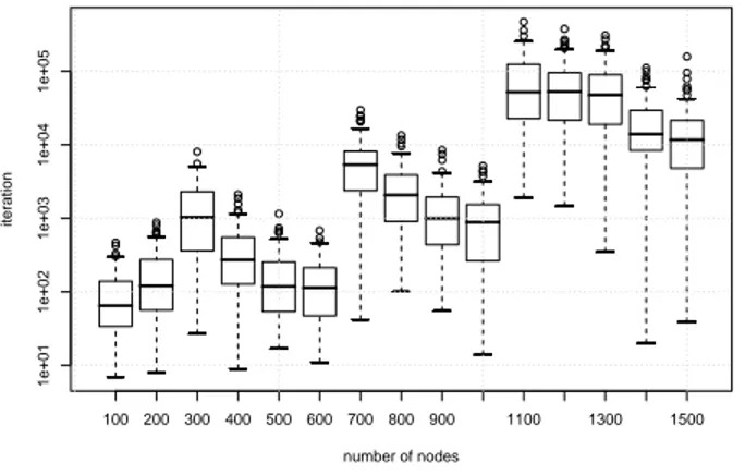
Fig. 4 and Fig. 5 summarize with standard box-and-whisker plots the medians, the quartiles, and the outliers of the iterations by EXPPLAT-RAND. Fig. 4 shows that there are some instances which are significantly harder than others. The sawtooth trend of the plot is due to the fact that EXPPLAT-RANDneeds on average more iterations to solve instances of the Gilbert model corresponding to the increase of the expected clique size in Table 1. Instances become then easier when the number of nodes increases and the maximum clique remains of the same size. This is confirmed also by all other algorithms considered.

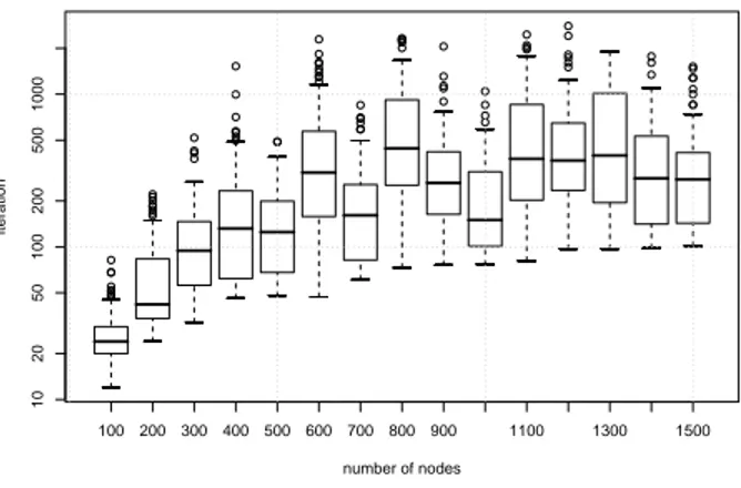
The sawtooth behavior is hardly visible in Fig 5 because of the different granularity of the cliques dimension with respect to the graph sizes considered.

100 200 300 400 500 600 700 800 900 1100 1300 1500 1e+01 1e+02 1e+03 1e+04 1e+05 number of nodes iteration

Figure 4: Iterations of EXPPLAT-RAND to find the empirical maximum clique in

100 200 300 400 500 600 700 800 900 1100 1300 1500 10 20 50 100 200 500 1000 number of nodes iteration

Figure 5: Iterations of EXPPLAT-RAND to find the empirical maximum clique in

P AT (n, n/3). Y axis is logarithmic.

3.2

Results summary

Because of lack of space, Table 2 presents the results on two specific instances of random graphs:GIL(1100, 0.3) and P AT (1100, 366). The choice of GIL(1100, 0.3)

is determined by the fact that it is empirically the most difficult instance of our data set, whileP AT (1100, 366) is chosen with the same number of nodes. The results

presented in Table 2 and discussed later are for 100 runs on 10 different instances.

GIL(1100, 0.3) P AT (1100, 366)

Algorithm Iter. Cost (µs) Iter. Cost (µs)

EXP-RAND [92%]* 9.00 [0%]* 3.80 EXP-STATDEGREE [0%]* 8.20 [40%]* 3.90 EXP-DYNDEGREE [10%]* 226.70 [0%]* 27.75 EXPPLAT-RAND 74697 6.40 273 3.50 EXPPLAT-STATDEGREE [60%]* 6.20 189 3.40 EXPPLAT-DYNDEGREE 75577 52.25 191 14.65 DLS-MC(pd=2) 75943 6.50 423 3.65 DLS-MC(pd=4) 63467 6.50 [99%]* 3.65 DLS-MC(pd=8) 73831 6.50 [85%]* 3.70 EXPPLATPRO.-RAND(T=2) 65994 6.50 310 3.60 EXPPLATPRO.-RAND(T=4) 67082 6.40 333 3.60 EXPPLATPRO.-RAND(T=8) 67329 6.30 329 3.60 RLS 49456 9.56 75 5.10 RLS-STATDEGREE 44588 6.95 86 4.70

Table 2: Results summary with the medians of the empirical steps distribution and the average time per iteration. (*) The algorithm is not always able to find the maximum clique; success ratio is reported.

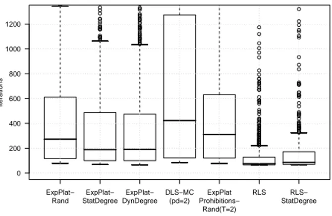
iterations 0 200 400 600 800 1000 1200 ExpPlat− Rand ExpPlat− StatDegree ExpPlat− DynDegree DLS−MC (pd=2) ExpPlat Prohibitions− Rand(T=2) RLS RLS− StatDegree

Figure 6: Iterations to find the empirical maximum clique inGIL(1100, 0.3). Results

for the most significant algorithms are reported.

3.3

Degree vs Penalties

From Table 2, it is clear that algorithms based only on greedy expansions are not always able to find the maximum clique in the given iteration bound, especially on hard instances. The plateau phase increases the success rate by reducing dramatically the iterations and therefore achieving the expected result within the iterations bound. Not surprisingly the introduction of the degree evaluation in the selection of the candidates is effective in the Preferential Attachment model, while in Gilbert’s graphs, where the nodes tend to have similar degrees, penalty- or prohibition-based algorithms win. The reduction in iterations achieved by EXPPLAT-STATDEGREE over EXPPLAT-RAND

onP AT (1100, 366) is about 31%. On GIL(1100, 0.3) DLS-MC(pd=4) finds the

maximum clique on average with 15% less iterations than EXPPLAT-RAND.

On the contrary, algorithms using degree information have poorer performances on Gilbert’s graphs, if compared with their completely random counterparts. For example

EXPPLAT-STATDEGREEfinds the maximum clique inGIL(1100, 0.3) only in the 60%

of the runs. The same can be noticed for penalty and prohibition-based algorithms whose performance is worse than EXPPLAT-RAND in the Preferential Attachment

model.

Table 2 shows also that selections based on dynamic degree are worsening the algorithm performance in most cases, leading to parts of the search space not containing the maximum clique. This is true also for RLS and RLS-STATDEGREE, which in any case find the maximum clique in less iterations on average than all the other algorithms.

3.4

Penalties vs Prohibitions

As shown in Table 2, DLS-MC is not always able to find the best clique onP AT

graphs while prohibition-based heuristic is always successful. Our results confirm that the penalty heuristic tends to be less robust than the prohibition-based heuristic. A significant dependency between DLS-MC performance and the choice of the penalty

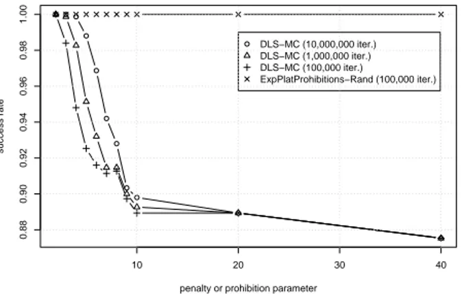
delay parameter is also discussed in [16]. Further investigations, summarized in Fig. 7, show the success rate of DLS-MC compared with that of EXPPLATPROHIBITION -RANDfor different values of the penalty delay and prohibition time parameters. The tests are on all instances of theP AT graphs of our data set.

EXPPLATPROHIBITION-RANDis always able to find the maximum clique within

100,000 iterations, while DLS-MC fails for several penalty delay values even incrementing the maximum number of iterations by a factor of 10 or 100.

10 20 30 40 0.88 0.90 0.92 0.94 0.96 0.98 1.00

penalty or prohibition parameter

success rate

DLS−MC (10,000,000 iter.) DLS−MC (1,000,000 iter.) DLS−MC (100,000 iter.)

ExpPlatProhibitions−Rand (100,000 iter.)

Figure 7: Success ratio of penalty- and prohibition-based algorithms on instances of the Preferential Attachment model.

3.5

Cost per iteration

The average CPU time per iteration is measured empirically by running the algorithm for 100,000 iterations and computing the time spent by a single iteration. The measure is repeated 10 times and averaged to reduce measurements errors.

The cost per iteration can therefore change significantly among different instances and it also depends on the directions taken in the search-space by the algorithms.

For example, the plateau phase does not only decrease the average number of iterations needed to find the maximum clique, but also the time spent by each single iteration. With a plateau phase, in fact, the less frequent restarts have a reduced impact on the average cost per iteration.

Table 2 shows that EXPPLAT-DYNDEGREEspends 47% less time per iteration than EXP-DYNDEGREE in P AT (1100, 366). The improvement is even bigger in GIL(1100, 0.3) where degree-based selections are less appropriate.

The reason for this reduction is that the algorithms spend most of their time in the expansion and plateau phases, more precisely updating incremental structures after a node has been added or dropped from the current clique. The complexity of the incremental update algorithm used in all the algorithms is bounded to the degree in the complementary graph of the node added or dropped from current configuration [7]. This is also the reason why the algorithms run faster on dense graphs. In case of

dynamic degree selection, the incremental update routine complexity depends also on the size of the POSSIBLEADDset. With plateau phases the search is longer and the

POSSIBLEADDset is on average smaller.

RLS, which has a different and less frequent restart policy, alternates between short expansions and plateaus. Therefore the POSSIBLEADDset remains on average smaller than in EXP-DYNDEGREE or EXPPLAT-DYNDEGREE and the cost per iteration is smaller.

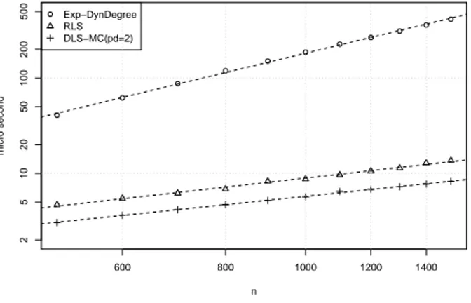
Fig. 8 shows the average CPU time per iteration on Gilbert’s graphs in log-log scale. The regression lines have a slope of 2.09, 0.98 and 0.90 respectively, confirming an approximate cost per iteration of EXPPLAT-DYNDEGREEgrowing asn2_{, while RLS,}

even having a candidate selection based on the dynamic degree, grows approximately linearly.

By multiplying the values in Table 2, the CPU time needed on average by

RLS-STATDEGREEto find the maximum clique in Gilbert’s hard instance is 63% of the

time required by DLS-MC(pd=2). RLS-STATDEGREEneeds 310 milliseconds while DLS-MC 494 milliseconds. 600 800 1000 1200 1400 2 5 10 20 50 100 200 500 n micro second Exp−DynDegree RLS DLS−MC(pd=2)

Figure 8: Empirical cost per iteration inµseconds on Gilbert’s graphs. Log-log scale.

4

Conclusions

The results of the tests on the instances of the two graph classes show clearly that the plateau search is necessary to find the maximum clique in hard instances and in any case to reduce the average number of iterations. The complexity added to the algorithms doesn’t increase the cost per iteration. On the contrary, especially for the algorithms using the dynamic degree for candidate selections, it reduces the CPU time per iteration.

On Gilbert’s graphs, where the nodes have the same degree on average, prohibition-or penalty-based algprohibition-orithms perfprohibition-orm better than pure random selections. On instances of the Preferential Attachment model, algorithms selecting the nodes using information about the degree are faster.

On the contrary, degree-based algorithms have poorer performance than random-selection algorithms in Gilbert’s graphs, while prohibition- and penalty-based algorithms are disadvantageous in the Preferential Attachment model. The penalty heuristic is less robust then the prohibition heuristic, depending on the appropriate selection of the panalty value.

RLS and RLS-STATDEGREE, always perform better then the other algorithms. The cost per iteration of RLS-STATDEGREEis similar to the one of DLS-MC, but the fewer steps needed on average to find the best cliques make it the best choice for the two graph models considered in this paper.

Acknowledgment

We thank Holger Hoos and co-authors for making available the software corresponding to the DLS-MC algorithm.

References

[1] A. L. Barabasi and R. Albert. Emergence of scaling in random networks. Science, 286:509 – 512, Oct 1999.

[2] Vladimir Batagelj and Ulrik Brandes. Efficient Generation of Large Random Networks. Physical Review E, 71(3):036113, Mar 2005.

[3] R. Battiti and M. Protasi. Reactive local search for the maximum clique problem. Technical Report TR-95-052, ICSI, 1947 Center St.- Suite 600 - Berkeley, California, Sep 1995.

[4] R. Battiti and G. Tecchiolli. The reactive tabu search. ORSA Journal on Computing, 6(2):126–140, 1994.

[5] Roberto Battiti and Alan Albert Bertossi. Greedy, prohibition, and reactive heuristics for graph partitioning. IEEE Transactions on Computers, 48(4):361– 385, Apr 1999.

[6] Roberto Battiti and Mauro Brunato. Approximation Algorithms and Metaheuristics, chapter Reactive Search: machine learning for memory-based heuristics. Taylor and Francis Books (CRC Press), 2006. in press.

[7] Roberto Battiti and Marco Protasi. Reactive Local Search for the Maximum Clique Problem. Algorithmica, 29(4):610–637, 2001.

[8] Eric Breimer, Mark Goldberg, David Hollinger, and Darren Lim. Discovering optimization algorithms through automated learning. In Graphs and Discovery, volume 69 of DIMACS Series in Discrete Mathematics and Theoretical Computer Science, pages 7–27. American Mathematical Society, 2005.

[9] S. Butenko and W. Wilhelm. Clique-detection models in computational biochemistry and genomics. European Journal of Operational Research, 2006. to appear.

[10] A. Grosso, M. Locatelli, and F.D. Croce. Combining swaps and node weights in an adaptive greedy approach for the maximum clique problem. Journal of Heuristics, 10:135–152, 2004.

[11] J. H˚astad. Clique is hard to approximate withinn1−ǫ_{. In Proc. 37th Ann. IEEE}

Symp. on Foundations of Computer Science, pages 627–636. IEEE Computer Society, 1996.

[12] Aric Hagberg, Dan Schult, and Pieter Swart, 2004. NetworkX Library developed at the Los Alamos National Laboratory Labs Library (DOE) by the University of California. Code available athttps://networkx.lanl.gov/.

[13] Frank Hutter and Youssef Hamadi. Parameter adjustment based on performance prediction: Towards an instance-aware problem solver. Technical Report MSR-TR-2005-125, Microsoft Research, Cambridge, UK, December 2005.

[14] Y. Ji, X. Xu, and G.D. Stormo. A graph theoretical approach to predict common rna secondary structure motifs including pseudoknots in unaligned sequences. Bioinformatics, 20(10):1591–1602, 2004.

[15] P.M. Pardalos and J. Xue. The maximum clique problem. Journal of Global Optimization, 4:301–328, 1994.

[16] Wayne Pullan and Holger H. Hoos. Dynamic Local Search for the Maximum Clique Problem. Journal of Artificial Intelligence Research, 25:159 – 185, Feb 2006.