UNIVERSITY
OF TRENTO
DIPARTIMENTO DI INGEGNERIA E SCIENZA DELL’INFORMAZIONE
38050 Povo – Trento (Italy), Via Sommarive 14
http://www.disi.unitn.it
NEIGHBORHOOD COUNTING MEASURE METRIC AND
MINIMUM RISK METRIC: AN EMPIRICAL COMPARISON
Andrea Argentini and Enrico Blanzieri
October 2008
1
Neighborhood Counting Measure Metric and
Minimum Risk Metric:
An empirical comparison
Andrea Argentini
1, Enrico Blanzieri
2Abstract—Wang in a PAMI paper proposed Neighborhood
Counting Measure (NCM) as a similarity measure for the k-nearest neighbors classification algorithm. In his paper, Wang mentioned Minimum Risk Metric (MRM) an earlier method based on the minimization of the risk of misclassification. However, Wang did not compare NCM with MRM because of its allegedly excessive computational load. In this letter, we empirically compare NCM against MRM on k-NN with k=1, 3, 5, 7 and 11 with decision taken with a voting scheme and
k=21 with decision taken with a weighted voting scheme on
the same datasets used by Wang. Our results shows that MRM outperforms NCM for most of the k values tested. Moreover, we show that the MRM computation is not so probihibitive as indicated by Wang.
Index Terms—Pattern Recognition, Machine Learning,
k-Nearest Neighbors, distance measures, MRM, NCM. I. INTRODUCTION
T
HE k-nearest neighbors (k-NN) is a well-known algorithm used in machine learning and in pattern recognition for classification tasks [1]. Given a point to classify and a distance (or similarity) function defined on the input space, k-NN finds the k-neighbors of the point and classify it to the majority class of its neighbors. The performance of k-NN depends on the distance/similarity function used to compute the set of neighbors and on the choice of k. The classification decision can weight the vote of each neighbor depending on the values of the used distance or similarity. In literature, there is a large variety of distance functions that are applicable to different data types. Among the most simple distances we can recall the Euclidean distance for numeric attributes and the Hamming distance for categorical attributes. More complex distances, such as HEOM [2] and HVDM [2], were introduced for data with mixed features. Other relevant distances are Minimum Risk Metric (MRM) [3] that minimize the risk of misclassification using conditional probabilities and Neighboring Counting Measure (NCM) proposed by Wang [4] that works counting the neigborhoods in the input space. Paredes and Vidal [5] presented an algorithm to learn weighted metrics for numerical data. The weights are learned by minimizing an approximation of the leave-one-out classification error on a subset of the training set with gradient descent algorithm. Dipartimento di Ingegneria e Scienza dell’Informazione , Universit`a di Trento, ItalyEmail : [email protected], [email protected]1
MRM is a distance for classification tasks that relies on the estimates of the posterior probabilities to minimize directly the misclassification risk. MRM builds on the approach started by Short and Fukunaga [6] metric that minimize the difference between finite risk and asymptotic risk. MRM uses a Na¨ıve Bayes to estimate the conditional probabilities for this reason the time of execution is high but as showed in [3] MRM outperformed other distance metrics like HEOM, DVDM, IVDM and HVDM. Despite its name, MRM is not a metric because it does not verify the identity of indiscernibles.
NCM [4], presented by Wang, works on the concept of neighborhood instead of neighbor. Once defined a topological space, the neighborhoods are regions in the data space that include a specific data point in a query. The similarity between two points is given by the number of neighborhoods that cover both points. In order to assess which points are closer to a test point NCM counts the neighborhoods and chooses the points that have more neighborhoods that are common with the test point. There are many ways to define a topological space. Wang defines the topological neighborhoods as a hypertuple and derive a method for counting in an efficient way all the possible neighborhoods. NCM can work with mixed-feature datasets, namely with both numerical and categorical features. NCM is simple to implement and has a polynomial complexity in the number of attributes. In [4] NCM is shown to outperform HEOM, DVDM, IVDM and HVDM, however, Wang did not test NCM against MRM for its high computational cost. In this way the author left unasked the questions on the comparison of the two methods.
In this letter, we compare the performance of NCM and MRM completing the comparison that was missing in [4]. Empirical evaluation shows that MRM outperforms NCM and, although the running time of MRM is higher, but in the same order of the running time of NCM and so it is not prohibitive as Wang suggested. The comparison between MRM, NCM and the technique by Paredes and Vidal [5] is beyond the aim of the present letter.
The paper is organized as follows: Section 2 overviews MRM and the similarity measure NCM. Experimental evaluation procedures and results are presented is Section 3. Finally, conclusions are drawn in Section 4.
II. METHODS
In this section we describe the methods tested in the experimental procedure.
A. Minimum Risk Metric
MRM proposed by Blanzieri and Ricci [3], is a very simple distance that minimizes the risk of misclassification r(x,y) defined as the ”the probability of misclassifying x by the 1-nearest neighbor rule given that the 1-nearest neighbor of x using a particular metric is y”. MRM is expressed by:
M RM (x, y) = r(x, y) =
m
X
i=1
p(ci|x)(1 − p(ci|y)) (1)
where m is the number of classes p(ci|x) is the probability that
x belong to the class ciand (1−p(ci|y)) is the probability that
the point y does not belong to the class ci. Given a point x and
a point y, respectively belonging one to the test set and one to the training set, the risk to misclassify x when assigning it the same label of y is given by p(ci|x)(1−p(ci|y)). The total finite
risk is the sum of the risks extended to all different classes like in (1). Several estimations of the conditional probabilities in (1) are possible so MRM can be considered a family of distances. A simple choice is to estimate the conditional probabilities p(ci|x) using the Na¨ıve Bayes estimator. The
idea of minimization of the expected risk as a distance has been more recently re-proposed by Mahamud and Herbert [7] who defined r(x, x0) as the ”conditional risk of assigning
input x with the class label corresponding to x0”. They also
demonstrated the optimality of it in terms of minimization of the expectation of r(x, x0) over the sampling of test points and
learning points. They pointed out that the (1) holds only in the case the samples are identically and independently distributed. Instead of estimating the risk by means of estimation of ˆp(x|ci)
in (1) they estimate r(x, y) directly as a function of a distance
d. From their work we can derive that MRM is symmetric,
subadditive (the triangular inequality holds), but it does not verify the identity of indiscernibles (namely M RM (x, y) = 0 iff x = y does not hold true) so MRM is not a metric but only a distance.
B. Neighborhood Counting Measure
The NCM proposed by Wang [4] is a similarity measure defined as: N CM (x, y) = n Y i C(xi, yi)/C(xi) (2) where C(xi, yi) = (max(ai) − max(xi, yi))×
(min(xi, yi) − min(ai)), if ai is numerical
2mi−1, if a i is categorical and xi= yi 2mi−2, if a i is categorical and xi6= yi (3) c(xi) = ½
(max(ai) − xi) × (xi− min(ai)) if ai is numerical
2mi−1, if a
i is categorical
(4) Where n is the number of attributes of the data, ai indicates
the i-th attribute and mi is defined as mi = |domain(ai)|,
finally xi, yi indicate the value of the i-th attribute in x and y
respectively. In (2) each factor in the product is the number of
DATASETS USED IN THE EXPERIMENTS.
DataSet Instances N Att Clas Val Type Missing
anneal 898 38 5 Mixed no
auto 205 25 6 Mixed no
breast-cancer 286 9 2 Mixed yes
bridges-v1 108 11 6 Mixed yes
credit-rating 690 15 2 Mixed yes
german-credit 1000 20 2 Mixed yes
zoo 101 17 7 Mixed no
credit 490 15 2 Mixed yes
hepatitis 155 19 2 Mixed yes
horse-colic-data 368 22 2 Mixed yes
bridges-v2 108 11 6 Nominal yes
vote 435 16 2 Nominal yes
tic-tac-toe 958 9 2 Nominal no
soybean 683 35 19 Nominal yes
audiology 226 69 24 Nominal no
primary-tumor 339 17 22 Nominal yes
sonar 208 60 2 Numerical no vehicle 846 18 4 Numerical no wine 178 13 3 Numerical no yeast 1484 8 10 Numerical no ecoli 336 7 8 Numerical no Glass 214 9 7 Numerical no heart-statlog 270 13 2 Numerical no pima-diabetes 768 8 2 Numerical no ionosphere 351 34 2 Numerical no iris 150 4 3 Numerical no
27 Dataset: 10 Mixed, 6 Nominal , 10 Numerical
neighborhoods for the i-th attribute.The NCM similarity has linear complexity with respect to the number of attributes. The idea underlying (2) is to count the neighborhoods between two points, where neighborhoods are defined basing on the notion of hypertuple. If the j-th attribute is categorical the number of neighborhoods is derived by the number of subsets that cover both points, otherwise if the j-th attribute is numerical the number of neighborhoods is represented by the number of in-tervals that generate a hypertuple that covers both points. Wang first develops the algorithm for counting the neighborhoods for categorical attributes and numerical attribute with finite domain. NCM as expressed in (2) is more general, and it takes into account also numerical attributes with infinite domain and it assumes the attributes to be equally important. The original paper did not mention how to manage the exceptions derived by 0/0 in (2) but following the indication of the author [8] in case of 0/0 we set the ratio equal to 1. In our experiments, we have used the distance 1 − N CM (x, y) as indicated by the author [8].
III. EMPIRICALEVALUATION
The aim of the experiment is to empirically compare the performance of NCM and MRM in classification tasks using the k-NN algorithm. We do not include HEOM, VDM and the standard Euclidean and Hamming metrics in our experiments because both MRM [3] and NCM [4] has been already shown to outperform this metrics in terms of accuracy.
A. Experimental procedure
The k-NN is applied to NCM and MRM and the decision on the class is taken with a simple voting schema on the k neighbors; in one specific case (with k=21) the decision is
3
taken with a weighted voting schema. In order to reproduce the results of [4] we considered the same datasets. Table I shows the datasets used. All of them originated from UCI machine learning repository [9]. The datasets have heteroge-neous composition (Nominal, Numerical, and Mixed), in order to evaluate the performance in datasets with different kind of features. The datasets used in [4] show some little difference in terms of number of attributes and number of instances. In particular Anneal, Credit and Soybean differs in the numbers of instances, whereas Vote, Zoo and Horse-colic differs in the number of attributes.
We ran 10-fold cross-validation 10 times with random partitions of data for each data set and for each k value. In each test we assess the statistical differences using the two-tail paired t-Test with significance level equal to 0.05. In order to compare directly with the data published by Wang [4] in a first set of experiments we set k = 11, and k = 21 with the weighted voting scheme. MRM is a distance function so we used as weight its inverse 1/distance whereas for NCM we used as weight directly the similarity value. We also run tests with the usual values of k=1, 3, 5, 7. We implemented both methods in Java and we used Weka [10] to perform all the tests, the statistical analysis and the measures of the running time. The Na¨ıve Bayes used in MRM is the one provided by Weka with numeric attributes that have been discretized replicating the choice done in [3]. In the training phase we create an hash table containing the estimates of ˆp(ci|y), with
y belonging to the training set. In this way, we compute a priori
the estimates of conditional probabilities for the training set. All the code and the datasets used in our tests are available on request.
B. Results and Discussion
The results of the experiments are presented as follows. Table II presents the results of k-NN with NCM and MRM and k=11, Table III presents the results with k=21 and the weighted voting scheme. Tables IV-V present the results with
k=1, 3, 5, 7. The tables present the statistical significance
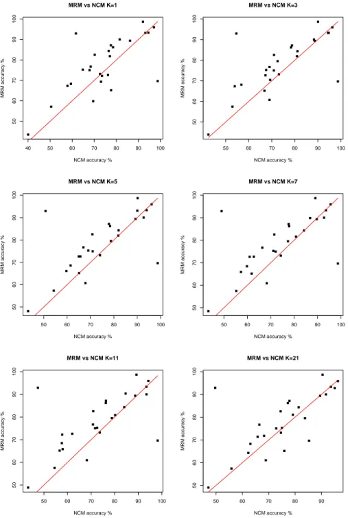
of the difference of the accuracy of MRM against NCM. In order to show visually the differences between the methods, Fig. 1 report scatter plots of the accuracies of MRM against NCM. Finally, Table VI shows a representative example of the running time of the two methods.
1) Reproducing NCM results: We compared the results for
NCM of Tables II-III with the analogous results presented by Wang. The variations in the selection of the folds of the datasets can account for the differences in the accuracies between our results and Wang’s, however, the differences are in the same order of the standard deviation so our results are substantially aligned with the results of NCM in its original proposal.
2) NCM vs MRM : MRM demonstrates good performances
in all the tests. Considering the number of datasets in which MRM has significative differences with respect to NCM, MRM is better than NCM, especially with k=11 and k=3. For example, with k = 1, MRM is significantly better of NCM in half of the datasets. These good results are also evident in the
TABLE II
ACCURACY RESULTS OFk-NNUSINGNCMANDMRMWITHk=11.
SIGNIFICATIVE DIFFERENCES ARE COMPUTED WITH RESPECT TONCM.
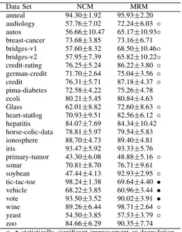
Data Set NCM MRM anneal 94.30±1.92 95.93±2.20 audiology 57.76±7.02 72.24±6.03 ◦ autos 56.66±10.47 65.17±10.93◦ breast-cancer 73.68±3.85 73.16±6.71 bridges-v1 57.60±8.32 68.50±10.46◦ bridges-v2 57.95±7.39 65.82±10.22◦ credit-rating 76.25±5.24 86.22±3.80 ◦ german-credit 71.70±2.64 75.04±3.56 ◦ credit 76.31±5.71 87.18±4.37 ◦ pima-diabetes 72.58±4.22 75.26±4.78 ecoli 80.21±5.45 80.84±4.63 Glass 62.01±8.82 72.60±8.63 ◦ heart-statlog 70.93±9.51 82.56±6.12 ◦ hepatitis 84.07±7.69 84.34±10.42 horse-colic-data 78.81±5.97 79.54±5.83 ionosphere 88.70±4.73 89.40±4.81 iris 93.47±5.92 93.33±5.76 primary-tumor 43.30±6.08 48.88±5.16 ◦ sonar 70.81±8.70 76.71±9.61 soybean 47.44±4.13 92.93±2.95 ◦ tic-tac-toe 98.24±1.38 69.64±4.40 • vehicle 68.22±3.85 60.96±3.44 • vote 93.50±3.52 90.02±3.91 • wine 89.26±6.44 98.71±2.64 ◦ yeast 54.50±3.85 57.53±3.79 ◦ zoo 84.66±6.29 90.35±7.74 ◦, • statistically significant improvement or degradation
TABLE III
ACCURACY RESULTS OFk-NNUSINGNCMANDMRMWITHk=21AND
WEIGHTED VOTING SCHEME. SIGNIFICATIVE DIFFERENCES ARE
COMPUTED WITH RESPECT TONCM.
Data Set NCM MRM anneal 96.27±1.57 95.87±2.22 audiology 68.24±7.65 71.79±6.15 autos 75.91±8.94 65.17±10.93• breast-cancer 74.64±4.00 73.16±6.71 bridges-v1 63.05±7.94 68.24±10.01 bridges-v2 62.26±9.08 64.29±9.35 credit-rating 77.26±5.22 86.22±3.80 ◦ german-credit 72.83±2.91 75.04±3.56 credit 77.88±5.57 87.18±4.37 ◦ pima-diabetes 75.02±4.54 75.26±4.78 ecoli 79.17±4.76 81.05±4.82 Glass 65.80±8.15 71.38±8.62 heart-statlog 74.52±7.83 82.56±6.12 ◦ hepatitis 81.38±6.01 84.34±10.42 horse-colic-data 83.77±5.69 79.54±5.83 ionosphere 89.52±4.72 89.40±4.81 iris 93.60±5.76 93.33±5.76 primary-tumor 47.08±5.20 49.03±5.26 sonar 66.43±8.10 76.71±9.61 ◦ soybean 49.69±4.18 92.91±2.95 ◦ tic-tac-toe 85.31±2.99 69.64±4.40 • vehicle 68.90±3.73 61.05±3.46 • vote 91.72±4.00 90.02±3.91 wine 90.45±5.98 98.71±2.64 ◦ yeast 55.84±3.64 57.37±3.70 zoo 95.05±6.24 92.81±6.95 ◦, • statistically significant improvement or degradation
scatter plots in Fig. 1. Considering all the results in Tables IV-V we can observe that increasing the value of k the only three datasets in which NCM reaches an accuracy significantly higher than MRM are Vote, Tic-Tac-Toe and Vehicle. This result is not surprising given the optimality of the minimization of the risk as a distance for classification tasks [7].
The running time results in Table VI show that the running time of MRM is in the same order of the running time of NCM. NCM is always faster of MRM except in the datasets
ACCURACY RESULTS OFk-NNOFNCMANDMRMWITHk=1ANDk=3. SIGNIFICATIVE DIFFERENCES ARE COMPUTED WITH RESPECT TONCM. k=1 k=3 Data Set NCM MRM NCM MRM anneal 97.04 ±1.75 95.95±2.19 96.31±1.74 95.95±2.19 audiology 76.23±7.64 72.64±6.10 67.25±7.60 72.64±6.10 ◦ autos 77.63±8.90 65.17±10.93• 66.80±10.43 65.17±10.93 breast-cancer 72.62±6.02 73.16±6.71 73.09±4.92 73.16±6.71 bridges-v1 59.43±11.45 68.31±10.90◦ 56.79±10.69 68.10±10.23◦ bridges-v2 57.87±11.61 67.32±11.16◦ 53.92±11.30 67.33±10.99◦ credit-rating 78.51±4.76 86.22±3.80 ◦ 78.35±4.73 86.22±3.80 ◦ german-credit 67.85±4.41 75.02±3.58 ◦ 70.89±3.33 75.01±3.59 ◦ credit 77.53±5.16 87.18±4.37 ◦ 78.76±4.54 87.18±4.37 ◦ pima-diabetes 64.82±6.28 75.26±4.78 ◦ 67.55±5.65 75.26±4.78 ◦ ecoli 77.08±6.24 81.84±4.70 ◦ 80.95±5.58 81.93±4.67 Glass 73.05±8.64 69.34±8.22 69.29±8.40 70.45±8.39 heart-statlog 70.22±9.31 82.56±6.12 ◦ 70.96±8.07 82.56±6.12 ◦ hepatitis 76.54±7.45 84.34±10.42 81.15±8.30 84.34±10.42 horse-colic-data 73.53±8.10 72.22±16.83 72.53±6.71 79.54±5.83 ◦ ionosphere 86.22±5.27 89.40±4.81 88.69±4.58 89.40±4.81 iris 94.53±5.56 93.33±5.76 94.73±5.22 93.33±5.76 primary-tumor 40.03±6.32 43.48±6.31 42.45±5.42 43.86±5.64 sonar 68.40±8.90 76.71±9.61 69.00±9.01 76.71±9.61 soybean 61.69±4.86 92.94±2.92 ◦ 54.60±4.25 92.94±2.92 ◦ tic-tac-toe 98.73±1.15 69.64±4.40 • 98.73±1.15 69.64±4.40 • vehicle 69.53±3.66 59.80±3.97 • 69.00±4.45 60.74±3.88 • vote 81.54±5.79 90.02±3.91 ◦ 88.32±4.92 90.02±3.91 wine 92.07±6.03 98.71±2.64 ◦ 90.10±6.04 98.71±2.64 ◦ yeast 50.48±3.81 57.14±4.09 ◦ 52.90±4.06 57.45±3.80 ◦ zoo 93.18±6.71 93.21±7.35 94.45±6.37 93.21±7.35
◦, • statistically significant improvement or degradation
TABLE V
ACCURACY RESULTS OFk-NNOFNCMANDMRMWITHk=5ANDk=7. SIGNIFICATIVE DIFFERENCES ARE COMPUTED WITH RESPECT TONCM.
k=5 k=7 Data Set NCM MRM NCM MRM anneal 96.15±1.47 95.95±2.19 95.59±1.54 95.95±2.19 audiology 65.71±8.24 72.64±6.10 ◦ 60.97±7.71 72.64±6.10 ◦ autos 65.15±10.48 65.17±10.93 61.82±10.91 65.17±10.93 breast-cancer 74.07±3.81 73.16±6.71 74.31±3.96 73.16±6.71 bridges-v1 61.50±9.54 68.59±10.69 59.82±8.28 68.42±10.70◦ bridges-v2 59.70±9.96 66.10±11.26◦ 57.26±9.14 65.90±10.76◦ credit-rating 78.39±4.77 86.22±3.80 ◦ 77.86±4.83 86.22±3.80 ◦ german-credit 70.94±3.10 74.93±3.54 ◦ 72.10±2.96 74.93±3.54 credit 77.88±5.21 87.18±4.37 ◦ 77.65±5.51 87.18±4.37 ◦ pima-diabetes 69.06±5.41 75.26±4.78 ◦ 71.12±4.77 75.26±4.78 ◦ ecoli 81.90±5.72 81.93±4.61 80.80±5.56 81.63±4.47 Glass 64.98±8.88 72.64±8.64 ◦ 62.75±8.90 72.69±8.57 ◦ heart-statlog 70.81±8.56 82.56±6.12 ◦ 71.52±8.68 82.56±6.12 ◦ hepatitis 82.03±8.42 84.34±10.42 84.20±8.48 84.34±10.42 horse-colic-data 78.75±6.06 79.54±5.83 77.39±6.48 79.54±5.83 ionosphere 89.24±4.27 89.40±4.81 89.66±4.33 89.40±4.81 iris 94.00±5.48 93.33±5.76 93.60±5.52 93.33±5.76 primary-tumor 43.33±5.84 48.20±6.20 ◦ 43.33±5.93 48.49±5.56 ◦ sonar 66.98±8.88 76.71±9.61 ◦ 66.40±7.92 76.71±9.61 ◦ soybean 50.79±4.43 92.94±2.92 ◦ 48.99±4.51 92.94±2.92 ◦ tic-tac-toe 98.73±1.15 69.64±4.40 • 98.73±1.15 69.64±4.40 • vehicle 67.85±3.79 60.71±3.91 • 68.27±3.79 60.86±3.57 • vote 92.74±3.50 90.02±3.91 • 92.81±3.94 90.02±3.91 • wine 90.15±6.15 98.71±2.64 ◦ 89.08±6.49 98.71±2.64 ◦ yeast 54.30±4.12 57.34±3.86 ◦ 55.25±4.16 57.45±3.80 zoo 90.03±6.59 93.11±7.32 86.85±6.83 89.85±7.54
◦, • statistically significant improvement or degradation
Breast-cancer and Vote where MRM has a smaller running time. However, the differences of running time between the two methods are not impressive. We can conclude that the computation of MRM is not prohibitive, far from the results of being ten times slower than NCM reported by [4] for a straightforward implementation. Wang did not report running times so it is not possible a comparison. It is important to note that the only improvement in our implementation with respect to a straightforward implementation is that we compute the estimates ˆp(ci|y) for y in the training set only once.
IV. CONCLUSION
We have presented an empirical comparison of MRM and NCM. The motivation for the empirical comparison arises from the fact that Wang in [4] did not performed the com-parison arguing the MRM was computationally heavy. Our comparison shown that MRM outperforms NCM. MRM, with a simple implementation has a computational cost slightly bigger than NCM, does not have a cost prohibitively high as the work by Wang suggested.
5 40 50 60 70 80 90 100 50 60 70 80 90 100 MRM vs NCM K=1 NCM accuracy % MRM accuracy % 50 60 70 80 90 100 50 60 70 80 90 100 MRM vs NCM K=3 NCM accuracy % MRM accuracy % 50 60 70 80 90 100 50 60 70 80 90 100 MRM vs NCM K=5 NCM accuracy % MRM accuracy % 50 60 70 80 90 100 50 60 70 80 90 100 MRM vs NCM K=7 NCM accuracy % MRM accuracy % 50 60 70 80 90 100 50 60 70 80 90 100 MRM vs NCM K=11 NCM accuracy % MRM accuracy % 50 60 70 80 90 50 60 70 80 90 100 MRM vs NCM K=21 NCM accuracy % MRM accuracy %
Fig. 1. Scatterplots of the accuracies of Tables II-V. MRM vs NCM for k=1, 3, 5, 7, 11, 21.
REFERENCES
[1] B. V. Dasarathy, Ed., Nearest Neighbor Pattern Classification
Tech-niques. IEEE Computer Society Press, 1991.
[2] D. R. Wilson and T. R. Martinez, “Improved heterogeneous distance functions,” J. Artif. Intell. Res. (JAIR), vol. 6, pp. 1–34, 1997. [3] E. Blanzieri and F. Ricci, “A minimum risk metric for nearest neighbor
classification,” in Proc. 16th International Conf. on Machine Learning. Morgan Kaufmann, San Francisco, CA, 1999, pp. 22–31.
[4] H. Wang, “Nearest neighbors by neighborhood counting,” IEEE Trans.
Pattern Anal. Mach. Intell, vol. 28, no. 6, pp. 942–953, 2006. [Online].
Available: http://doi.ieeecomputersociety.org/10.1109/TPAMI.2006.126 [5] R. Paredas and E. Vidal, “Learning weighted metrics to minimize
nearest-neighbor classification error,” IEEE Transactions on Pattern
Analysis and Machine Intelligence, vol. 28, no. 7, pp. 1100–1110, 2006.
[6] R. Short and K. Fukanaga, “The optimal distance measure for nearest neighbor classification,” IEEE Trans. Information Theory, vol. 27, pp. 622–627, 1981.
[7] S. Mahamud and M. Hebert, “Minimum risk distance measure for object recognition,” in ICCV. IEEE Computer Society, 2003, pp. 242–248. [Online]. Available: http://csdl.computer.org/comp/proceedings/iccv/2003/1950/01/195010242abs.htm [8] H. Wang, “Personal communication,” 2007.
[9] C. L. Blake and C. J. Merz, “UCI repository of machine learning databases,” 1998, http://www.ics.uci.edu/∼mlearn/MLRepository.html. [10] I. H. Witten and E. Frank, Data Mining: Practical machine learning
tools and techniques. Morgan Kaufmann San Francisco, 2nd Edition 2005.
RUNNING TIME IN SECONDS FOR THE TEST PHASE OFk-NNUSING THE
TWO METHODS WITHk=1.
Data Set NCM MRM anneal 1.46±0.65 2.62±0.87 audiology 0.15±0.03 1.02±0.37 autos 0.05±0.02 0.19±0.07 breast-cancer 0.06±0.03 0.03±0.02 bridges-v1 0.01±0.00 0.01±0.00 bridges-v2 0.01±0.00 0.01±0.00 credit-rating 0.32±0.05 0.29±0.08 german-credit 1.14±0.38 0.85±0.31 credit 0.16±0.04 0.22±0.13 pima-diabetes 0.08±0.03 0.32±0.19 ecoli 0.02±0.00 0.09±0.03 Glass 0.01±0.02 0.04±0.02 heart-statlog 0.02±0.01 0.02±0.01 hepatitis 0.01±0.00 0.02±0.01 horse-colic-data 0.14±0.04 0.13±0.07 ionosphere 0.08±0.05 0.25±0.10 iris 0.00±0.01 0.01±0.00 primary-tumor 0.17±0.06 0.44±0.11 sonar 0.06±0.03 0.24±0.72 soybean 0.86±0.10 4.10±0.16 tic-tac-toe 0.52±0.21 0.41±0.02 vehicle 0.32±0.13 0.96±0.36 vote 0.20±0.08 0.10±0.02 wine 0.01±0.00 0.02±0.03 yeast 0.43±0.13 2.82±0.98 zoo 0.02±0.00 0.01±0.00
Andrea Argentini received a B.Sc degree in com-puter science from the University of Bologna in 2004 and he received a M.Sc.degree in computer science, with emphasis in bioinformatics, from the University of Trento in 2008. He is currently a Phd student in machine learning and bioinformatics at the University of Trento. His research interests include data mining, machine learning, and bioinformatics.
Enrico Blanzieri received the Laurea degree (cum laude) in electronic engineering from the University of Bologna in 1992, and a Ph.D. in cognitive science from the University of Turin in 1998. From 1997 to 2000 he was researcher at ITC-IRST of Trento, and from 2000 to 2002 he was assistant professor within the Faculty of Psychology of the University of Turin. Since 2002 he is assistant professor at the Department of Information and Telecommuni-cation Technologies of the University of Trento. His research interests include soft computing, artificial intelligence and bioinformatics.