RICERCA DI SISTEMA ELETTRICO
Minimizing temperature difference in HVAC systems for high
energy efficiency in buildings
(IEA – ECBCS Annex 59)
M. Perino, V. Serra, S. P. Corgnati, E. Fabrizio, F. Favoino, S. Fantucci
DIPARTIMENTO ENERGIA
Report RdS/2012/ 117
Agenzia nazionale per le nuove tecnologie, l’energia e lo sviluppo economico sostenibile
MINIMIZING TEMPERATURE DIFFERENCE IN HVAC SYSTEMS FOR HIGH ENERGY EFFICIENCY IN BUILDINGS (IEA – ECBCS ANNEX 59)
M. Perino, V.Serra, S. P. Corgnati, E.Fabrizio, F. Favoino, S.Fantucci (Politecnico di Torino Dipartimento Energia)
Settembre 2012
Report Ricerca di Sistema Elettrico
Accordo di Programma Ministero dello Sviluppo Economico – ENEA Area: Razionalizzazione e risparmio nell’uso dell’energia
Progetto: Studi e valutazioni sull’uso razionale dell’energia: Tecnologie per il risparmio elettrico nel settore civile
Indice
Sommario ……….………...4
Introduzione……….4
Descrizione delle attività svolte, risultati, discussione e
pubblicazioni……… …....7
Approfondimento 1………10
Approfondimento 2………..….30
Approfondimento 3……….………..44
Conclusioni……….46
Appendice……….……….….47
Sommario
I temi sviluppati nell’ambito del presente progetto sono parte del più ampio progetto della International Energy Agency -ECBCS Annex 59 “Minimizing Temperature Difference in HVAC Systems for High Energy Efficiency in Buildings”, approvato dall’Executive Committee nel mese di Ottobre 2011. Il gruppo di ricerca TEBE (www.polito.it/tebe) del Dipartimento di ENERGIA del Politecnico di Torino ha avuto un ruolo propositivo e attivo nella definizione dei contenuti del progetto, fin dalla sua fase di concezione, partecipando agli incontri preliminari tra il nucleo dei proponenti e contribuendo alla scrittura del progetto stesso.
In questa fase di start-up del progetto, l’attività dell’unità di ricerca del Politecnico di Torino ha focalizzato il proprio specifico approfondimento sui sistemi per il riscaldamento ambientale basati su impianti solari termici che utilizzano fluidi e sistemi innovativi (con particolare riferimento a materiali a cambiamento di fase fluidizzati, “Slurry PCM”). Questa fase della ricerca è risultata essenziale per cominciare aa individuare le effettive possibilità applicative, nonché i limiti, di queste soluzioni tecnologiche integrate. Parallelamente, è stato condotto un approfondimento sulle potenzialità applicative dei pannelli radianti per la climatizzazione accoppiati a sistemi impiantistici operanti a temperatura moderata. Il tema guida della ricerca può essere sintetizzato nell’analisi delle potenzialità applicative di nuovi sistemi integrati del sistema edificio-impianto che interagiscono con la fonte energetica solare.
Gli studi condotti sono propedeutici allo sviluppo di uno specifico modello di calcolo per il progetto di sistemi impiantistici per la climatizzazione, in particolare utilizzanti la tecnologia radiante, in presenza di elevati carichi solari.
Introduzione
L’attività di ricerca condotta è strettamente correlata al programma dell’ Annex 59 dell’IEA (International Energy Agency) “High Temperature Cooling & Low Temperature Heating in Buildings”.
Al fine di inquadrare al meglio le linee di approfondimento del progetto, si riportano di seguito alcuni estratti del documento che illustra il progetto stesso.
“The purpose of buildings and HVAC systems is to maintain suitable indoor climate quality, including required levels of temperature, humidity and indoor air quality. Theoretically, any heating source with a higher temperature than the indoor environment can supply heat in winter and vice versa for cooling sources in summer. Since the temperature of heating sources and cooling sources influences HVAC energy consumption directly, high temperature cooling and low temperature heating has the potential to increase energy efficiency. The concept of reducing the temperature difference between heating sources/cooling sources and the indoor environment typically involves increasing the dimensions of heat exchange surfaces. Independent control of temperature and humidity is another important aspect of high temperature cooling and low temperature heating.
[...] the proposed project is organized following the idea of reducing mixture loss and transfer loss, and the work subtasks are arranged in response to the current insufficiency or inadequateness of HVAC system.
The main objectives of the research proposal can be summarized as three aspects:
- Establish a methodology for analysis of the thermal environment system from the perspective of reducing mixture loss and transfer loss.
The ultimate goal of the Annex is hence to:
Build up the concept of surveying HVAC system from the perspective of reducing mixture loss and transfer loss then apply it in analysis of actual energy saving technologies
To reach this goal, an international collaboration is needed on different issues: a deep and comprehensive investigation to evaluate current situation, summarize the appropriate and inappropriate design of HVAC systems, unify and clarify the research methodology, discuss on basic settings and methodology of simulation and testing, research on key parameters of radiant terminals, study energy saving potential and limitation of radiant terminals combined with fresh air system, research on HVAC indoor terminals for large space building, including radiant floor and supply air terminals.
La struttura dell’Annex 59 è riportata nella figura 1 allegata.
Descrizione delle attività svolte, risultati, discussione e
pubblicazioni
Relativamente ai sistemi per il riscaldamento ambientale basati su impianti solari termici che utilizzano fluidi e sistemi innovativi, in questa prima fase delle attività, il lavoro del gruppo di lavoro del Politecnico di Torino si è organizzato su tre fronti distinti:
analisi della configurazione impiantistica di base, analisi e selezione dei fluidi di processo,
creazione di un profilo temporale “tipo” di carico termico e sviluppo di un modello numerico semplificato per il pre-dimensionamento della superficie captante e dell’accumulo termico.
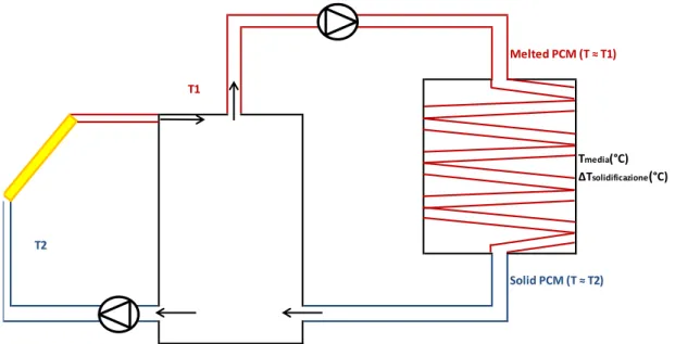
Il primo fronte ha riguardato la concezione degli schemi di impianto (collettore-circuito primario-accumulo-circuito secondario) da associare al collettore solare a materiale a cambiamento di fase fluidizzato in progetto. In particolare si è svolto uno studio specifico in relazione ai fluidi da adottare per i vari circuiti (slurry-PCM sul primario, slurry-PCM sul primario e secondario con scambiatore intermedio, slurry-PCM sul primario e secondario senza scambiatore intermedio), pervenendo a due schemi tipo riassunti nei disegni seguenti (figure 2 e 3). Melted PCM (T ≈ T1) T1 Tmedia(°C) ΔTsolidificazione(°C) T2 Solid PCM (T ≈ T2)
Figura 2 - Schema di impianto solare termico con due circuiti a slurry-PCM aperti.
Figura 3 - Schema di impianto solare termico con due circuiti a slurry-PCM chiusi e scambiatore intermedio
Nel primo schema di impianto i due circuiti (primario e secondario dell’utenza) sono collegati idraulicamente all’accumulo sotto forma di slurry-PCM. Il materiale viene fuso nel passaggio nel collettore e, successivamente (se la radiazione solare è sufficientemente alta), passa dalla temperatura T2 alla temperatura T1. Sull’utenza il materiale subisce la solidificazione e ritorna all’accumulo sotto forma di solido (sospeso in fase liquida).
Nel secondo schema, invece, il circuito primario è collegato idraulicamente all’accumulo mentre il circuito secondario dell’utenza è dotato di uno scambiatore intermedio annegato nell’accumulo. Il funzionamento è analogo a quello dello schema precedente con la differenza che in questo caso può essere adottato un fluido diverso per il circuito secondario (ad esempio acqua o uno slurry PCM con caratteristiche termo fisiche diverse da quello del primario). Da un punto di vista puramente termotecnico il caso migliore e più efficiente è rappresentato dal primo schema poichè utilizza un circuito aperto per la carica e lo scarico dell’accumulo. Senza l’utilizzo di uno scambiatore, la quantità di energia termica che può essere trasferita all’utenza è maggiore.
Tuttavia, è raro che si possa utilizzare in utenze domestiche, ad esempio pannelli radianti a pavimento, la miscela acqua-slurry-PCM che presenta una densità maggiore dell’acqua, anche perche i PCM microincapsulati potrebbero in qualche punto dell’impianto danneggiare o ostruire le tubazioni. L’opportunità di utilizzare il PCM fluidizzato anche sull’utenza dovrà essere oggetto di ulteriori studi, pertanto si e deciso di adottare il secondo schema di impianto con scambiatore intermedio sull’accumulo. Certamente questo secondo schema di impianto risulta essere meno efficiente del primo in quanto nello scambio di energia termica viene “perso” un salto di temperatura di circa 2- 3 °C.
Il secondo fronte di attività ha riguardato la selezione del materiale a cambiamento di fase (PCM) fluidizzato più adatto per l’impiego all’interno del collettore solare. Questo studio, riportato nel dettaglio nell’approfondimento 1, ha preso in esame come primo elemento la
immagazzinabile nella miscela acqua + PCM micro incapsulato da utilizzarsi in progetto in funzione sia del calore specifico del materiale in esame, sia della temperatura media di lavoro rispetto alla temperatura dell’utenza.
Il terzo fronte ha consentito di ottenere un profilo di richiesta termica (ottenuto mediante simulazione numerica con il software Energy Plus). Sulla base di questa informazione è quindi stato possibile andare a simulare il comportamento di massima del sistema captatore accumulo termico e andare ad indagare l’effetto della variazione della temperatura di fusione/solidificazione del materiale a cambiamento di fase fluidizzato sull’accumulo di energia termica stagionale, la massimizzazione della frazione solare e la funzionalità dell’impianto. Nello specifico la creazione numerica di un profilo orario di domanda di energia termica per riscaldamento da associare al collettore solare in progetto è descritta nell’approfondimento 2. Il profilo orario di richiesta termica per riscaldamento è stato sviluppato per l’intera stagione invernale, per un alloggio tipo equipaggiato con pavimenti radianti e collocato nel clima di Torino. A valle della calibrazione dei risultati di simulazione, il profilo così ottenuto è stato utilizzato per valutare le necessità di accumulo termico in funzione di diversi livelli termici impostati (a seguito della selezione del materiale slurry-PCM) andando a fare un’analisi di sensibilità sulle principali variabili del sistema (numero di pannelli, temperatura di lavoro, ecc.) Sono stati altresì raccolti profili di richiesta di energia termica per riscaldamento reali da utilizzarsi nella simulazione del comportamento del collettore solare in progetto.
Con specifico riferimento ai sistemi per il controllo climatico basati su concetti mirati alla minimizzazione delle differenze di temperatura, i risultati ottenuti e presentati in questa relazione si possono schematizzare nei seguenti punti:
- individuazione del concetto di schema impiantistico su cui basare la futura sperimentazione (vi è l’intenzione di realizzare, in collaborazione con aziende del settore, un dimostratore le cui prestazioni saranno successivamente monitorate), - Individuazione (ed acquisizione) del PCM micro incapsulato con sui realizzare lo slurry
PCM (fluido di processo),
- Creazione di un profilo temporale tipo (di riferimento) della domanda termica (di riscaldamento) sulla cui base sviluppare analisi si sensitività per il dimensionamento/ottimizzazione del sistema impiantistico
- Simulazione – di massima – del comportamento del sistema solare a slurry PCM per individuare campi termici di funzionamento dell’impianto e dimensioni dei componenti principali.
L’attività di ricerca – al momento – è focalizzata alla progettazione e realizzazione di un circuito di laboratorio in cui misurare le proprietà termo fisiche dello slurry PCM che sarà successivamente utilizzato all’interno del dimostratore.
Si evidenzia che, poiché questa attività di ricerca è iniziata nel corso di questo anno, al momento non sono state ancora prodotte pubblicazioni di carattere scientifico. Si prevede di pubblicare alcuni risultati intermedi nel corso del prossimo anno
Parallelamente, è stato sviluppato uno studio rivolto all’esame delle potenzialità di applicazione dei pannelli radianti (pavimenti e soffitti) per la climatizzazione accoppiati a
temperatura moderata. In “Approfondimento 3” è riportato l’Abstract dell’articolo pubblicato nella rivista internazionale HVAC&R Research su tale tematica.
Le evoluzioni delle ricerche condotte sono indirizzate a mettere in luce le potenzialità applicative di nuovi sistemi integrati del sistema edificio-impianto che interagiscono con la fonte energetica solare.
Approfondimento N. 1
Analisi dei fluidi di processo e simulazione numerica di massima
del sistema solare termico innovativo
In this deliverable the different slurries phase change materials that are currently on the market are presented as a function of the fusion/solidification temperature, of the heat capacity coefficient and of the other thermophysical properties. Moreover, following the seasonal thermal load profile previously determined (annex 2), a comparison between the performance of a solar system with water and one with a mixture water-slurry PCM was done. Nel presente deliverable vengono indagate le diverse tipologie di fluidi a cambiamento di fase fluidizzati attualmente disponibili sul mercato in funzione della temperatura di fusione/solidificazione, del calore specifico e delle altre proprietà termofisiche. A seguito dell’analisi, a partire dai dati del profilo orario stagionale di potenza termica determinato nell’allegato 2, è condotto un confronto tra le prestazioni di un impianto solare funzionante ad acqua ed uno funzionante con miscela acqua-slurry-PCM.
PCM emulsions and mPCM slurries
A new technique has been proposed to use PCM materials in thermal storage systems: this technique consists of forming a two-phase mixture fluid, such as water and a phase change material, such as paraffin, resulting in a latent heat storage fluid. Inaba has classified thermal fluids, describing the main characteristics and applications. Among the latent thermal fluids, five types of fluids are mentioned: 1) ice slurries, 2) phase change material microemulsions, in which the PCM is dispersed in water through an emulsifying agent; 3) microencapsuled PCM slurries, where the PCM is microencapsuled in a polymeric capsule and dispersed in water; 4) clahrate hydrate PCM slurries, where the clahrate hydrates are composed of water molecules (host molecule) forming a weaved structure where the molecules of the other substance (guest molecule) are accommodated, constituting a special molecular structure where the heat associated with the chemical reaction of formation and dissociation of clathrate hydrate is greater than that of ice melting; 5) shape-stabilized PCM slurries (ssPCM slurries), this consist of paraffin unfilled in high density polyethylene, with a melting temperature higher than of the paraffin. In this way the paraffin is retained inside the high density structure polyethylene, avoiding the leak of the PCM. Different types of PCM slurries: (*the case of clathrate hydrate PCM slurries does not appear drawn, In 2010 Zhang et al. published a review about thermal properties and applications).
As main issues to be tackled, some studies inform that in the case of mPCM slurries it is particularly difficult to maintain a stable homogeneous flow if the particles are not processed with very small size and high flexibility.
Fig.1. Schematic drawing of the different types of PCM slurries
Besides the PCM capsules entails an extra cost, the capsule prevents the PCM in continuous phase from leaking, which in that case could solidify in ducts and cause clogging. It is important that the capsules are sufficiently resistant against the stress produced by pumps. In the case of emulsions, instabilities could appear during phase change and that is difficult to maintain a stable emulsion above melting temperature. Stratification problems will appear as the paraffin droplets will form grater droplets and finally a PCM layer will float in the upper part of the storage system, due to the difference of densities.
Advantages of these new fluids as thermal storage materials or heaters transfer fluids: 1) High storage capacity during phase change
2) Possibility to use the same medium either to transport or store energy (as theses slurries are pumpable), reducing in this way heat transfer losses.
3) Heat transfer at an approximately constant temperature. 4) High heat transfer rate due to higher heat capacity.
5) A better cooling performance than conventional heat transfer fluids, due to the decrease in fluid temperature as a consequence of higher heat capacity.
6) A better thermal energy storage density in comparison to conventional systems of sensible heat storage in water and can be competitive against macroencapsuled PCM tanks.
In order to be advantageous these latent fluids must meet the following requirements: 1) High heat capacity
3) Low subcooling 4) High heat transfer rate
5) Pumpable, low pressure drop in pumps systems 6) Stable over a long term storage
7) Stable at thermal-mechanical loads in pump systems.
Fabrication of PCM microcapsules
Microencapsulation: in recent years this technique widely used in the pharmaceutical and chemical engineering fields, has reached the field of phase change materials in order to improve their behavior. The most utilized techniques for PCM microencapsulation are: the spraydrying technique, coacervation, in situ, interfacial polymerization. (*These three methods are explained on the article ‘Review on phase change material emulsions and microencapsulated phase change material slurries: Materials, heat transfer studies and
applications’)
PCM microcapsules and mPCM slurries studied in literature
Microencapsulation Process Core Material Shell Material Melting Temperature (ºC)
Phase change entalpy (kJ/kg)
In situ polymerization Tetradecane PS (poliestirene) 2,06 0 In situ polymerization Tetradecane PMMA (Polymethyl methacrylate) 5,97 66,26 In situ polymerization Tetradecane Polyethyl methacrylate 5,68 80,62 Interfacial polymerization n-Octadecane Melamine formaldehyde 24 -
In situ polymerization Paraffin Ura-formaldehyde 54 157,5 Polymerization of emulsion Docasane PMMA (Polymethyl methacrylate) 41 54,6
In situ polymerization n-Octadecane Melamine formaldehyde 30,5 170 Polymerization n-Octacosane PMMA (Polymethyl methacrylate) 50,6 86,4 Coacervation/Spray-drying Paraffin wax
(Merck) - - 145/240
In situ polymerization n-Octadecane Melamine formaldehyde 40,6 144 Coacervation n-Octadecane - 24-29 147,1
These two tables show only some of the PCM studied materials with their properties and the obtaining methods, extracted of the article ‘Review on phase change material emulsions and microencapsulated phase change material slurries: Materials, heat transfer studies and applications’ where others are also shown.
Fig.2. Microencapsulation process PCM Emulsifying method Surfactant
Melting Temperatu
re (ºC)
Phase change entalpy (kJ/kg)
Mixture of n-alkanes Ultrasonic generator Non-ionic surfactant 9,5 78,9
20% Tetradecane Phase inversion
6% surfactant (67,7%Tween60 and 32,3%Span60) - 43 Tetradecane (10% ) 5,06 (10% ) 18,5 (20% ) 5,84 (20% ) 112,3 (30% ) 5,84 (30% ) 150,8 Mixture of hexadecane and tetradecane 70/30 and 2,5% paraffin as nucleation agent 1,5% alcohol ethoxylate (30%RT6) 75 (30%RT10) 50 (30%RT20) 44 Paraffin RT10 Phase incursion 4 - 11,5 55
Fig.3. Drying Process Commercially available PCM microcapsules
Main characteristics of PCM emulsions and mPCM slurries
Solidification, hysteresis and subcooling
Instabilities problems (PCM emulsions) due to:
- Creaming or sedimentation- Flocculation
- Coalescence
- Ostwald ripening - Phase inversion
Instabilities problems (mPCM slurries) due to:
- Microcapsule rupture (*Yamagishi studied the damage produced by the stress caused by the pump or by agitation on microcapsules.
Viscosity values. PCM emulsions and mPCM slurries studies in literature
A) Dispersion system
B) Water
Thermal properties. Thermal conductivity
The low thermal conductivity is one of the main disadvantages of thermal energy storage systems with PCMs. Some values are shown in the next table:
The low thermal conductivity results in slow charging and discharging. Are numerous studies aimed at the improvement of the thermal conductivity of the PCM. The way to do that could be by embedding structures of materials with high thermal conductivity or by using finned heat exchangers or encapsulating the PCM in containers with a high surface/volume ratio. This is the reason why PCM microcapsules are interesting. Due to the microscopic size of the PCM microcapsules or droplets, the PCM slurry can be treated as a homogeneous material. This assumption implies in that the temperature gradients inside the solid are negligible. This is accomplished if the convective thermal resistance inside the microcapsules is low in comparison the convective thermal resistance between the microcapsule and surroundings. PCM slurries in water can improve heat transfer as a consequence of the relationship area/volume of droplets in the case of emulsions and of microcapsules in the case of slurries, in comparison to systems in which the PCM is macroencapsulated. Besides, the fact of dispersing phase change particles into a fluid can improve heat transfer through convection with respect to water. These slurries can serve either as thermal storage materials or heat transfer fluids. The thermal properties of these slurries are different from those of PCM and the fluid in question, which are essential to evaluate the fluid and the heat transfer characteristics of a system with these slurries. The thermal properties to be discussed are thermal conductivity and convection heat transfer coefficient. The analysis of the different studies regarding the convection heat transfer coefficient is presented in a separate section, due to their extension and importance within this review.
Kasza and Chen studied and documented the benefits of the use of PCM slurries in water, such as the improvement in heat transfer and increase in storage efficiency. Some of the benefits mentioned are:
1) Reduction in the temperature difference between source and drain
2) Increase of heat capacity of the fluid, as a consequence of the PCM dispersion. This gives place to a lower mass flow and therefore an a lower pumping consumption. 3) Dynamic use of the PCM. In a conventional system, heat exchange between PCM
(static use) and a separated heat transfer fluid is need to transport heat or cooling. With PCM slurries, thermal storage and the heat transfer fluid are integrated into the PCM slurry.
Improvement in heat transfer occurs in slurries, with or without phase change. This improvement is substantially greater when considering PCM slurries.
Compilation of studies carried out on the heat transfer phenomenon in PCM
emulsions and mPCM slurries
PCM slurries
Objectives magnitudes and influential parameters at the time or selection of a PCM emulsion or mPCM slurry as heat transfer fluid or thermal storage material.
Applications
The main application present in literature is the utilization of PCM emulsions and mPCM slurries and thermal storage materials and heat transfer fluids in chilled ceilings.
-Wang and Niu presented the results of a mathematical simulation of a combined system of chilled ceiling and storage tank with a mPCM slurry, in addition to an air treatment unit for the ventilation necessities, in a room with the climatology of Hong Kong. During working hours, the mPCM
slurry flowed from the tank to the chilled ceiling, melting the PCM and releasing the latent heat. The combination of the chilled ceiling plus storage tank against a conventional water system achieved peak shaving, and therefore a smaller cooling unit/chiller could be sufficient. The consumptions were practically the same for the mPCM slurry and water. Nevertheless, it
must be taken into account that calculations were carried out using the same COP for the case of the tank with water and mPCM slurry, when in reality the COP for the case of the tank with mPCM slurry is higher due to operation at lower environment temperatures (charging during the night).
-Griffiths and Eames studied experimentally the pumping of a mPCM slurry from BASF manufacturer through a chilled ceiling in a room. The room was tested during four months with a 40% PCM concentration. When water was pumped through the chilled ceiling, a mass flow of 0.7 l/s was required for an inlet temperature of 16 ◦ C and outlet temperature of 18 ◦ C, maintaining the room at 19 ◦ C. When water was substituted by the mPCM slurry, the slurry was capable of maintaining a temperature of 20–21 ◦ C with a mass flow of 0.25 l/s. This means that the ceiling required a lower mass flow (pumping savings were not quantified), could absorb energy at a constant temperature, avoiding increments in the panel surface temperature when internal gains increased.
-Another well-known application, similar to the previously described, was carried out at the Narita Airport in Tokio by Shibutani . The issue in the installation of the Narita Airport in Tokio was the change of refrigerants due to environmental reasons. When R11 and R22 were substituted by R134a and R123 without changing the chiller unit, this resulted in lower cooling power and the
chiller was non-capable to absorb the demand peaks at specific times of the day. This problem was solved through the installation of a tank filled with a mPCM slurry custom-developed by Mitsubishi Heavy Industries. The characteristic temperatures on the demand side were a supply temperature of 5 ◦ C and a return flow temperature of 12 ◦ C. A mPCM slurry was selected with a phase change temperature range between 5 and 8 ◦ C. The demand peaks occurred between 8:00 and 22:00, and therefore the cooling produced during the night by the chiller unit could be stored and reduce the
demand peaks during the day. The slurry presented a storage density of 67 MJ/m3, lower in comparison to an ice tank, 167 MJ/m3, but higher in comparison to water, 21 MJ/m3. Both the COP of the system and the operational costs for water and mPCM slurry were similar and lower than the ice tank.
The main part of the information of this report has been obtained from the paper:
‘Review on phase change material emulsions and microencapsulated change material slurries: Materials, heat transfer studies and applications’
Authors: Mónica Delgado , Ana Lázaro, Javier Mazo, Belén Zalba
Aragón Institute for Engineering Research (I3A), Thermal Engineering and Energy Systems Group, University of Zaragoza, Spain
Solar circuit simulation - Parametric Data Analysis
A parametric real time simulator has been created, leading us to simulate all the cycle performance depending on the input conditions at each interval of time. It will represent a good overview of how the circuit will perform and which are going to be the decisive variables on it.
Moreover, it will allow us to appreciate the technological feasibility of the project. Taking inputs such as the number of solar collectors and the accumulator dimensioning as a starting point, several values can be determined: the amount of demand that can be covered (solar fraction), the quantity of mixture stored at a specific time in the tank and the energy loss the system is not able to take benefit from, for example.
From here on, a reasonable decision should be made about which the optimum number of solar collectors and the accumulator volume will be. Nevertheless, the circuit system should not only be chosen to cover the maximum heating demand. It is also important to consider other aspects such as the size of the accumulator and capacity to emplace it, the quantity of
fluid or mixture needed to be stored and to flow through the circuit, the overall cost of the heating system, among others.
This simulator also shows a good approximation of how the charge and discharge of the accumulator tank will be depending on each mean hour weather conditions of the flat’s placement (Torino – Italy).
Pursuing all these issues, the program created is based on some constant and modifiable inputs:
Constant inputs Modifiable inputs
- Mean hourly outdoor dry bulb temperature (T∞) - Number of solar collectors - Mean hourly radiation received per m2 of collector at
operational inclination (GT)
- Accumulator sizing
- Mean temperature of the mixture at the solar collector (Tm)
- Constant parameters and features of the solar collector
The mean hourly constant outputs (dry bulb temperature and radiation received on a reference collector of 1m2) are outputs obtained from the EnergyPlus simulation and the weather conditions introduced.
Simulation features and variables - Collector characterization
The instantaneous efficiency of the solar collector is needed to assess an estimation of the heating production at real time. It provides the basis for simulation models of thermal processes and for setting up the procedure for assessing the collector performance.
Data such as radiation received per m2 of collector at a specific inclination (GT), ambient
temperature (T∞) and wind speed are recorded and allow the characterization of a collector by
parameters that indicate how the collector absorbs energy and how it loses energy to the surroundings.
The next equation for is a nonlinear expression also used in “Energy balance of the flat plate solar collector” section. It was firstly formulated by Cooper and Dunkle (1981). In this equation the instantaneous efficiency is referred as a function of the arithmetic average of the fluid inlet and outlet temperatures (Tm) and also of the overall loss coefficient (UL). The values of the
constant parameters ( , a1 and a2) are given by the manufacturer of the collector and were
displayed before in page 14 with other features.
This method is the basis of standard EU collector efficiency formulation.
Where, is the mean fluid temperature difference and it is calculated as:
The values of corresponding to each timestep were obtained from the EnergyPlus simulation by implementing a reference surface at the operational inclination and with the same dimensions than the selected solar collector. Thus, the program exhibited the values of mean hourly radiation received per m2 that our solar collector would have received throughout all the simulation period.
operational conditions. Its assigned values, when the flowing fluid is water or when it is only PCM, are 55°C and 37°C, respectively.
Note: Only two study cases were simulated. The first system used water as the flowing fluid and the second system one used a fluid consisting only on the selected PCM. The second case is obviously not real, since the PCM is not able to flow by itself. Water in a good proportion is needed to ensure the correct flowing of the mixture through the circuit. However, in these first steps of the project, experimental tests to determine which would be the best density of the mixture and therefore the proportions of the water-PCM mixture to be implemented have not been developed yet. From this approach, the first hypothetical system using water represents the performance of the system as the reference one, which is already being applied nowadays. The second hypothetical case should be understood as an ideal system that only uses PCM. Thereby, the real case performance would be found in an intermediate point in between those two.
Solar collector instantaneous efficiency ( ) The instantaneous efficiency ( ) was assessed as:
If (by Eq. of page 45)
Where represents the value of solar radiation from which no useful energy gain can be produced. That is:
Energy production (Wh)
The solar collector energy production was assessed as:
If
Where the total amount of solar radiation received was calculated as: N: Number of solar collectors used (modifiable input)
: Effective collector area Energy demand (Wh)
The energy demand was obtained for each timestep as an EnergyPlus output (Plant Loop Heating Demand (Wh)).
Accumulated energy (Wh)
The accumulated energy represents the energy that may be stored in the storage tank or accumulator for each timestep. Defining a variable X as:
And knowing that the initial value of accumulated energy at the starting point of the simulation is 0, the accumulated energy was assessed during the rest of the performance as:
If
If
The sum of the immediately previous value of energy accumulated ( ) and the actual energy production may supply the actual energy demand. If it does not occur, the rest of the demand which have not been supplied will be named as “not satisfied demand”. From this approach, the assessment of the not satisfied demand was:
If
Loss energy (Wh)
The energy loss represents the energy that cannot be stored in the accumulator when there is too much production. It was calculated as:
If
Simulation analysis and discussion
The most significant parameters are the number of solar collectors and the accumulator sizing. The number of solar collectors limits the energy production and therefore the energy accumulated, facing a constant demand. The total energy production should be, at least, equal or higher than the total energy demand. For this reason, the number of solar collectors that produces more than the 2310.09 kWh demanded throughout all the simulation period, was checked. It was found that five solar collectors were the minimum number of solar collectors needed to satisfy the total energy demand. On one hand, if any accumulator was used, only a 9.56% of the total energy demand would be supplied. On the other hand, the 60% of the total heating demand would be satisfied if a huge accumulator of 13.000 L of water was used. In the first case, all the energy produced during one hour must be consumed in the same hour (hourly values of production, demand, accumulation and losses); if not, this energy produced becomes an energy loss. The presence of the accumulator and its dimensions properly calculated are important and relevant factors of the system performance. The accumulator should be dimensioned to cover the maximum energy demand (or solar fraction) as possible, but always satisfying restrictive parameters. For instance, these limit values could be the overall cost or the space to emplace the tanks. A commonly applied circulating fluid flow in heating systems that use water as fluid is of ca. 50 or 75 L of fluid per m2 of solar collector. This value can serve as reference in the sizing of the accumulator tank.
The number of solar collectors may be also limited, either by the overall cost or by the available surface on the top of the building to emplace them. The latter issue has been studied deeply.
Assuming that a building with other apartments like the studied and a top roof building area of 130.06m2, the assessment of the maximum number of solar collectors that can be emplaced there is shown in the following lines:
The minimum distance between solar collectors to avoid that one line of collectors doesn’t block out the sun to the next one is:
Figure 4. Sketch of the minimum distance between solar collectors
Therefore, a hypothetical distribution could be done in an overall roof surface of 11x12 m2 in which 15 solar collectors can be set up:
12m
11m L
d h
Figure 5. Sketch of a hypothetical distribution of the solar collectors
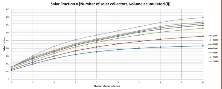
In order to decide the final number of solar collectors and the accumulator size, Fig. 6 shows the evolution of production and demand of one reference day.
Fig. 6 was developed to make a good decision about which the number of solar collectors and the volume of the storage tank would be.
- Y-axis: the solar fraction represents the energy demand supplied and it is the main reference parameter. The maximum value that it can take is 1, and it would correspond to the supply of all the heating demand.
- X-axis: number of solar collectors, from one to ten.
-
Finally, each curve corresponds to a specific storage volume of the accumulator tank.Fig. 6 is a very useful plot since the solar fraction can be understood as function of the number of solar collectors and the accumulator volume. Typical solar fractions for water heating systems are 0.5 – 0.75. Therefore, and trying not to oversize the tank and the number of solar collectors, the system would be properly sized with 7 or 8 solar collectors and an accumulator of 4000L.
The selected volume of 4000L is equal to 93kWh of energy that can be stored during all the simulation period.
Moreover, the optimum number of collectors would be eight and the corresponding solar fraction of 0.66. On the other hand, a solar fraction of 0.62 would be covered with seven solar collectors. Assuming that the building is composed by two apartments and eight solar collectors for each apartment, the total collecting surface will be of 18.8m2.
The simulation results for the selected configuration are shown in the next pages:
Selected configuration Number of solar collectors 8
Accumulator volume (L) 4000
- The total production represents the 165% (3827kWh) of the total energy demand. - The demand not satisfied represents the 33.6% (776.2kWh) of the total energy
demand.
- Energy losses that could not be stored represent the 57.5% (2200.2kWh) of the total energy production.
Note: In future studies, the high amount of loss energy should be deeply though as a new energy source that could be used to supply other energy demands. This energy is lost since the tank cannot store all the amount of energy produced. The stored energy is limited by the tank dimensions and the volume of fluid flowing.
Energy accumulated in the storage tank (hourly)
Demand not satisfied (hourly)
Figure 8. Plot of the demand not satisfied evolution
Fig. 8 displays the demand that cannot be supplied because of the low production and the dimensions of the accumulator tank. This demand, as it can be observed, is completely interrelated with the energy accumulated at each timestep. The periods with low values of energy accumulation and with high demand and low production are the periods when the largest amount of demand not satisfied is reached.
Loss energy (hourly)
Figure 9. Plot of the energy loss evolution
Fig. 9 displays the energy that cannot be stored because of the accumulator dimension. This energy, as it was explained before, represents the largest amount of energy losses and overlaps in periods of high production. On the other hand, during the coolest months of December, January and February no energy is lost, thus all the production is consumed.
Energy variables confrontation (daily)
Production vs Demand (daily)
Fig. 9 was developed in order to confront the following variables: accumulated energy, demand not satisfied, loss energy and energy demand. These have been simplified to a daily timestep instead of hourly. Therefore, every twenty four mean hourly values one average has been represented.
Fig. 10 displays the comparison of the mean daily production and the mean daily demand. It can be noted how 8th of January is the worst day of the simulation, being the demand at its highest value (42326.55W) and with no production at all. In the other hand, considering an ideal day with the largest production and energy demand is for instance, the 5th of March with an overall energy production of 48463.84W and an energy demand of 4446.51W. However, as it could be seen in the plot, it is not the most common situation.
Production vs Demand evolution during a day (hourly)
Furthermore, Fig. 12 focuses on how the production and energy demand perform during any day. The plotted day is the 25th of January, in which the production was larger than the demand.
Figure 12. Plot of the production and demand evolution during one day
Analysing the daily consumption and energy requirements of a normal family it is obvious that the energy demand curve may not follow the energy production curve. It would be ideal if the red curve was always under the blue one and, from this approach, the energy could be consumed in a short time after it is produced. However, this delay in the production is the real situation and to achieve the purpose of covering the maximum energy demand it is needed to store the rest of the energy produced when there is no consume or a low one. Thereby, it is demonstrated how necessary the accumulator tank is.
Comparative study between PCM - water
All the results of the previous section have been referred to a system which only uses water. Nevertheless, as objective of the project, the system will use a mixture of water and PCM in short time. Therefore, the current section tries to present an approximated result of what it would be obtained if the fluid circulating was the PCM-water mixture, but without knowing its
Comparison values for water and PCM systems
Water PCM % of PCM improvement from water case
Production 3827.06 5416.10 41.52
Not satisfied demand 776.22 464.54 -40.15
Accumulated energy 248810.57 293192.73 17.84
Energy loss 2200.17 3477.53 58.06
Final Conclusions
Production improvement responds to the low temperature at which the PCM works and absorbs heat in the solar collector. As it is shown in the Collector Efficiency, the collector efficiency is higher with low Tm temperatures.
Energy demand not satisfied has been reduced by a 40% compared to the water simulation. The production increase makes it possible to satisfy a larger amount of the energy demand. In an overall rate, the energy demand not satisfied in the water simulation represents the 33.6% of the total energy demand. On the other hand, the energy demand not satisfied in the PCM simulation represents the 20% of the total energy demand.
The accumulated energy increase by a 17.84% happens due to the property of the fluid to absorb more heat at a low temperature. It should be noted that the accumulator size remains the same as in the water simulation.
The energy loss increase also responds to the larger production and the limited accumulator size.
The main advantage of using a mixture of water and PCM compared to a system that only employs water as a circulating fluid is that energy can be stored in a larger amount. Therefore, the larger energy it is stored, the larger energy demand it can be satisfied. The mixture with PCM reduces the mean work temperature (Tm) and increases the solar collector efficiency.
Approfondimento N. 2
Determinazione del profilo orario tipico del carico termico di
riscaldamento
In this step of the project, the main objective was to determine the value of the energy demand in a specific house or apartment. To obtain that, an energy analysis and thermal load simulation program in buildings was used: EnergyPlus.
This software enables to model all kind of energy and mass flows as: heating, cooling, lighting, ventilation or water use. It also includes many simulation capabilities: time-steps less than an hour, modular systems and plant integrated with heat balance-based zone simulation, multizone air flow, thermal comfort, natural ventilation and photovoltaic systems.
Based on a building description, house or apartment, and on a weather file of the location, the program can calculate the heating and cooling loads necessary to maintain thermal control setpoints, the energy consumption of the primary plant equipment and the conditions throughout a secondary HVAC system and coil loads. Depth studies and continuous program improvements allowed us to think that EnergyPlus results are close to the real building ones. EnergyPlus has been designed to be a simulation engine, an element within a system of programs that includes a graphical user interface to describe the building.
The program needs various input files that describe the building to be modelled and the environment surrounding it. The program produces several output files, which need to be described or further processed in order to make sense of the results of the simulation. The results obtained after the simulation are showed in a spreadsheet for the postprocessor results files, in a web browser for the tabular results file and in a viewer for the selected drawing file.
Input Data File
The input data file (idf) is an ASCII file containing the data describing the building and the HVAC system to be simulated. All the description of the building is included in it and all its features could be created and modified.
An apartment divided in three zones where a family of 4 people lives and with a total area of 130.06m2 is going to be analysed. This flat is part of a building that has other flats like this, but our study case was simplified to one of them.
The flat has been subdivided in three zones. Each zone has a window that according to the Italian standards has a surface of at least 1/6 of the zone floor area. A solar collector of reference, with the same surface and inclination as the used one is exposed over the west zone.
The main structural features of the construction included in the input file are: dimensions, materials and construction, simulation period, weather file, internal gains and zone airflow.
Dimensions
1. Zones
Table 1. Zones dimensions
Zone Lenght [X](m) Widht [Y](m) Height [Z](m) Floor Area(m2)
West zone 6.10 6.10 3.05 37.16
East zone 6.10 6.10 3.05 37.16
North zone 9.14 6.10 3.05 55.74
Total Area(m2) 130.06
2. Windows
Table 2. Windows dimensions
Zone Lenght [X](m) Widht [Y](m) Height [Z](m) Window Area(m2)
West zone 3 - 2.1 6.30
East zone 3 - 2.1 6.30
North zone - 4.5 2.07 9.32
Total Area(m2) 21.92
Materials and Construction
The elements of the building (walls, floors, roofs and windows) will determine the interactions of the building surfaces with the outside environment parameters and the internal space requirements. These surfaces are also used to represent the heat transfer through zones. To simplify the model no doors have been included.
1. External walls
The external walls are exposed to the external environment. These are composed by five layers. The materials have been chosen following one typical Italian structure.
Note: The outside layer refers to the side that is not exposed to the zone but rather the opposite side environment, which can be the outdoor environment or another zone.
Figure 2. External walls
materials and distribution
2. Internal walls or partitions
Construction Material
Outside Layer External insulation Layer 2 Brick holed wall Layer 3 Polystyrene Layer 4 Brick wall Layer 5 Internal insulation
Material Internal gypsum Brick wall Ins-Expanded polystyrene
Holed brick
wall External gypsum
Roughness Smooth Rough Rough Rough Rough
Thickness(m) 0.1 0.08 5.00E-02 0.25 0.1
Conductivity(W/m·K) 0.9 0.3 3.00E-02 0.5 0.9
Density(kg/m3) 1600 725 56.06 1200 1800
Specific Heat(J/kg·K) 850 850 1210 850 850
*The Air gap filled by ‘F04 Wall air space resistance’ has a thermal resistance of 0.15
Table 4. Internal walls materials properties (II)
Material G01a 19mm gypsum
board Roughness MediumSmooth Thickness(m) 0.02 Conductivity(W/m·K) 0.16 Density(kg/m3) 800 Specific Heat(J/kg·K) 1090 3. Floor and Roof
In the simulation both have been considered as adiabatic surfaces. These are common surfaces between two zones, where both zones are typically at the same temperature. Thus, no heat transfer is expected in the surface from one zone to the next, but will store heat in thermal mass. Only the inside face of the surface will exchange heat with the zone.
Table 5. Floor and roof materials and their properties Construction:
Floor Material
Outside Layer F16 Acoustic tile Layer 2 F05 Ceiling air space resistance Layer 3 M14a 100mm heavyweight concrete
Construction Material
Outside Layer G01a 19mm gypsum board Layer 2 F04 Wall air space resistance Layer 3 G01a 19mm gypsum board
Construction:
resistance of 0.18
Material M14a 100mm
heavyweight concrete F16 Acoustic tile
Roughness MediumRough MediumSmooth
Thickness(m) 0.10 0.02
Conductivity(W/m·K) 1.95 0.06
Density(kg/m3) 2240 368
Specific Heat(J/kg·K) 900 590
4. Internal Source: Radiant Panels
The radiant panels are situated under the main floor of each zone.
Table 6. Internal sources materials and their properties
Construction: Internal Source Material
Outside layer Concrete - Dried sand and gravel 4 in Layer 2 Ins-Expanded polystyrene R12 2 in
Layer 3 GYP1
Layer 4 GYP2
Layer 5 Finishing flooring - Tile 1 / 16 in
Material
Concrete - Dried sand and gravel 4
in
Ins-Expanded polystyrene R12 2
in
GYP1 GYP2 Finishing flooring - Tile 1 / 16 in
Roughness MediumRough Rough MediumRough MediumRough Smooth
Thickness(m) 0.10 0.05 0.01 0.02 0
Conductivity(W/m·K) 1.29 0.02 0.78 0.78 0.17
Density(kg/m3) 2242.58 56.06 1842.12 1842.12 1922.21
Specific Heat(J/kg·K) 830 1210 988 988 1250
In the case of radiant systems, the construction has hydronic tubing embedded within the construction. The heat is then added to the building element to provide heating to the zone in question. The definition is similar to the Construction definition with a few additions related to radiant or other systems that will lead to source terms.
The source is present after layer number 4; therefore, it can be said that the source is located between the GYP2 layer and the Finishing flooring.
The temperature requested for the calculation is also checked after layer number 4. This allows us to calculate the temperature within the construction.
5. Windows
Table 7. Windows materials and their properties
Construction Material
Outside Layer LoE TINT 6MM
Layer 2 KRYPTON 8MM
Layer 3 LoE CLEAR 6MM Rev
Thickness(m) 0.01
Material: Glazing LoE TINT 6MM LoE CLEAR 6MM Rev
Optical Data Type SpectralAverage SpectralAverage
Thickness(m) 0.01 0.01
Solar transmitance at normal incidence 0.36 0.6
Front side solar reflectence at normal incidence 0.09 0.22
Back side solar reflectence at normal incidence 0.2 0.17
Visible transmitance at normal incidence 0.5 0.84
Front side visible reflectence at normal incidence 0.04 0.08
Back side visible reflectence at normal incidence 0.05 0.06
Infrared transmitance at normal incidence 0 0
Front Side Infrared Hemispherical Emissivity 0.84 0.1
Back Side Infrared Hemispherical Emissivity 0.1 0.84
Conductivity(W/m·K) 0.9 0.9
Simulation period
The run period selected has been from 15 of October to 15 of April, which includes the six months of heating demand by citizens of Torino (Italia).
Therefore, the total number of hours present in the simulation will be 4392. Weather file
The weather file is an ASCII file containing the hourly or sub-hourly weather data needed by the simulation program. A data record collected during many years allows the program to iterate and confront the input and the weather files, showing output meters and spreadsheets of results.
The weather file also contains the information about the location and climate. The specific flat is situated in Torino, capital of the Piemonte region in the northwest of Italy.
The location parameters are:
Table 8. Location parameters of the flat Location Torino - Italy
Latitude(deg) 45.22
Longitude(deg) 7.65
Elevation(m) 287
Some of the weather parameters available and modifiable that the iteration confronts and takes into account are, among others, listed below:
Design Conditions Typical/extreme periods Dry bulb temperature Dew point temperature
Wind speed Wind direction
Solar radiation (beam/diffuse) Sky cover
These parameters, among others, are defined in more detail at “Simulation Outputs” section. Internal gains
Other internal sources and equipments can influence the energy consumption of the flat. People, lights, electric equipment or slab floor may come into play.
1. People
The energy gains provided by people, as well as the level of carbon dioxide generated by these are calculated and taken into account in the simulation. The flat has a family of four people. The presence of people varies as a function of the schedules, but only four people can be found as maximum: one person in the West zone, one in the east zone and two in the North zone.
The presence or non-presence of people in the flat is controlled by the schedules introduced and it is represented by a fraction. This fraction will be the same for each zone (e.g. If the fraction is 1, in the West and East zones will be one person and in the North zone will be two persons).
The schedule for the house occupancy is shown below: - During weekdays:
Table 9. Schedule for the house occupancy Hour Interval Fraction
occupancy From Until 0:00h 6:00h 1 6:00h 7:00h 1 7:00h 8:00h 0.5 8:00h 12:00h 0 12:00h 13:00h 0.5 13:00h 16:00h 0 16:00h 17:00h 0.5 17:00h 18:00h 1 18:00h 24:00h 1
- The fraction occupancy during weekends, holidays and all other days for any time is 1
- The fraction occupancy for WinterDesignDay and holidays for any time is 1 2. Lights
The energy given by lights is another factor that must be considered as an energy gain. The lights power consumption is set in at most 5 W/m2 (per zone floor area).
The house lighting is also controlled by the schedules introduced and is represented by a fraction. This fraction will be the same for each zone.
The schedule for the house lighting is shown below: - During weekdays:
Table 10. Schedule for the house lighting Hour Interval Fraction
lighting From Until 0:00h 6:00h 0.1 6:00h 7:00h 0.2 7:00h 8:00h 0.6 8:00h 12:00h 0 12:00h 13:00h 0.5 13:00h 16:00h 0 16:00h 17:00h 0.5 17:00h 18:00h 0.6 18:00h 24:00h 0.8
- The house lighting during weekends, holidays and all other days for any time is 0.8 - The fraction lighting for WinterDesignDay and holidays for any time is 1
3. Electric equipment
The electric equipment such as television, computers, fridge and others electric appliance also contribute to the heat zone loads and therefore in increasing the mean temperature of each zone. The electric consumption is set in at most 10 W/m2 (per zone floor area). The house lighting is also controlled by the schedules introduced and it is represented by a fraction. This fraction will be the same for each zone.
The schedule for the electric equipment is shown below: - During weekdays:
Table 11. Schedule for the electric equipment Hour Interval Fraction
equipment From Until 0:00h 6:00h 0 6:00h 7:00h 0.5 7:00h 8:00h 1 8:00h 12:00h 0 12:00h 13:00h 0.5 13:00h 16:00h 0
- The electric equipment during weekends, holidays for any time is 0.8 - The electric equipment for WinterDesignDay and holidays for any time is 1
4. Radiant panels heating system
The radiant panels are the last energy gain which contributes in the indoor temperature. It is the most significantly factor of the internal energy gain. Under each zone floor there is a radiant panel (internal source) providing heat.
The radiant panels operation is controlled by two parameters, a first “switch on” temperature that represents the minor heating water loop temperature which should be not overcome. This has been fixed with the next values for each schedule:
Table 12. Radiant panels heating system schedule Hour Interval Heating
setpoint (°C) From Until 0:00h 7:00h 18 7:00h 17:00h 21 17:00h 24:00h 18
And a second “switch off” temperature that represents the maximum heating water loop temperature which should not be overcome. This has been fixed to every hour and every day of the simulation period with a value of 35°C. The European heating standards fix the maximum value of indoor floor temperature at 29°C, so the “switch off” water value takes this into consideration.
Zone airflow
Infiltrations can be understood as a heat loss, but all the zones should be ventilated. The infiltration value is specified as a design level which is modified by a schedule fraction, temperature difference and wind speed. The calculation method has been designed as Air Changes per hour, being this factor:
Simulation outputs
Each zone command generates zone outputs using the input fields above. The most common indoor and outdoor outputs are listed below:
Ambient environment outputs:
- Outdoor Dry Bulb (°C): The outdoor air dry-bulb temperature will be
used in other sections in order to calculate the overall heat loss coefficient, losses to the environment, the solar collector efficiency and the heating production. The outdoor dry-bulb temperature will be named in other sections as “Outdoor air temperature”.
- Outdoor Wet Bulb (°C): The outdoor wet-bulb temperature is derived
(at the timestep) from the values for dry-bulb temperature, humidity ratio and barometric pressure.
- Outdoor Humidity Ratio (kg water/kg air): The air humidity ratio
represents the mass of water vapour to the mass of dry air. It is unit less. - Wind Speed (m/s): The outdoor wind speed.
- Wind direction (degree): The outdoor wind direction (N=0, E=90,
S=180, W=270).
- Sky temperature (°C): The sky temperature is derived from horizontal
infrared radiation intensity. The program assess it as:
Where (Steffan-Boltzmann constant)
- Horizontal Infrared Radiation (W/m2): The horizontal infrared
radiation intensity is based on opaque sky cover, sky emissivity, temperature and other factors.
- Diffuse solar radiation (W/m2): Diffuse solar radiation is the amount
of solar radiation received from the sky (excluding the solar disk) on a horizontal surface.
- Direct (or beam) solar radiation (W/m2): Direct solar radiation is the
amount of solar radiation received within a 5.7° field of view centred on the sun. This is also known as beam solar.
Zone thermal outputs:
- Zone Mean Air Temperature (°C): This is the zone average
temperature of the air at the timestep. The zone heat balance supposes a well stirred model for a zone; therefore, there is only one mean air temperature to represent the air temperature for the zone. It is calculated for each zone.
- Hydronic Low Temp Radiant Heating Energy (J): This field reports the
heating input to the low temperature radiant system. This is the heat source to the surface that is defined as the radiant system. The heating rate is determined by the zone conditions, the control scheme defined in the user input, and the timestep. It is calculated for each zone.
- Hydronic Low Temp Radiant Water Mass Inlet Temp (C): This field
reports the temperature of water entering the low temperature radiant system. It is calculated for each zone.
- Hydronic Low Temp Radiant Water Mass Outlet Temp (C): This field
reports the temperature of water leaving the low temperature radiant system. It is calculated for each zone.
- Zone Total Internal Heat Gain (J): Theses report variables represent
the sum of all heat gains (radiant, convective and latent) from specific internal sources throughout the zone in watts (for rate) or joules. This includes all heat gains from: people, lights, electric equipment, gas equipment, hot water equipment and steam equipment and other equipment. It is calculated for each zone.
- Plant Loop Heating Demand (W): This field is not calculated for each
zone, but it is the overall assessment of the heating demand of the three zones. This is the net demand required to meet the heating setpoint of the loop. In the particular case of this study, as the loop setpoint is met for the current HVAC timestep, Plant Loop Heating Demand is equal to the sum of the total heating demand from the demand side coils on the loop, that is the same value which is obtained from summing the three Hydronic Low Temp Radiant Heating Energy values (J) (one from each zone) and dividing it by 3600 (to convert J into W). Some of the mentioned output values are plotted and analysed in the following pages in order to obtain an easy results overview.
Plant loop heating demand (hourly)
Figure 3. Plot of the plant loop heating demand along all the simulation period.
Note: There is no heating demand of the April period from 4152 to 4392 hour.
Heating demand frequency
Fig. 4 shows the hourly frequency of the heating demand at each power rate. This and the others plots performed were referenced to the six months of simulation (from 15th of October to 15th of April):
Table 13. Percentage of hours front the total of heating demand Heating Demand (Wh) Percentage of total hours (%) = 0 61.36 0 < HD ≤ 1000 22.36 1000 < HD ≤ 2000 6.67 2000 < HD ≤ 3000 3.85 3000 < HD ≤ 4000 2.37 4000 < HD ≤ 5000 2.39 ≥ 5000 1
The total number of hours that were considered by the simulation period was 4392 hours. Table 17 shows how the circuit will perform only a 38.64% of the time because there is no heating demand during a 61.36% of the period.
Figure 4. Plot of the total hours at each range of heating demand, when there is heating demand >
0.
The plant loop heating demand is distributed along the simulation period as shown in Fig. 3. From this approach, it could be noted that the main part of the demand is at low consume. Moreover, the number of hours at which the demand is higher than 4kWh only represents a 3.39% of the overall amount, in front of the resting 35.25%. The most common factor which enhances the low consume is that there is more demand under 1000Wh than over this value, 22.36% and 16.28%, respectively.
Zones mean air temperatures vs Outdoor air temperature
Fig. 5 displays how the average temperature of three zones starts with a value as high as 35°C, to decrease until a value of approximately 20°C during the first 20 days (500h). Then, it remains constant during the cooler months and increases again around the middle of March.
The indoor temperature remains constant, without huge variations, after it is achieved at home (about 5°C between day and night). This is not the case of the outdoor temperature. Although its temperature profile is similar to the one displayed by the indoor temperature, the variation between two close instants reaches values of 15 or 20°C. The small indoor variations are not only due to the heating system, but also because of the insulation layers of walls, roof and ground which conserve the internal gains and reduce the heat losses. Other internal gains as lights, people and electric equipment also contribute to the indoor temperature.
Moreover, the confrontation of mean air temperatures for each zone reveals that the West zone has the highest temperature profile during the simulation period, followed by the East zone. Thus, the North zone, that is the coolest one, has lower temperatures most of the time. This is the reason why the North zone heating system is active more time than at the other zones and why there it is reached the highest value of total mass flow.
The total mass flow values consumed by the radiant panels are shown below in Table 14:
Table 14. Total mass flow values consumed by the radiant panels Total mass flow
consumption (kg/s) West zone 9.88
East zone 11.82