THE ITALIAN OPTIMIZATION TOOL FOR
THE GAINS-ITALY MODEL
A. CIUCCI, L. CIANCARELLA, G. ZANINI
ENEA – Unità Tecnica Modelli, Metodi e Tecnologie per le Valutazioni Ambientali Laboratorio Qualità dell'Aria
Centro Ricerche “E. Clementel”, Bologna I. D’ELIA
ENEA - Unità Centrale Studi e Strategie Servizio Analisi e Scenari Tecnico-Economici
Sede Centrale, Roma
AGENZIA NAZIONALE PER LE NUOVE TECNOLOGIE, LʼENERGIA E LO SVILUPPO ECONOMICO SOSTENIBILE
THE ITALIAN OPTIMIZATION TOOL FOR
THE GAINS-ITALY MODEL
A. CIUCCI, L. CIANCARELLA, G. ZANINI
ENEA – Unità Tecnica Modelli, Metodi e Tecnologie per le Valutazioni Ambientali Laboratorio Qualità dell'Aria
Centro Ricerche “E. Clementel”, Bologna I. D’ELIA
ENEA - Unità Centrale Studi e Strategie Servizio Analisi e Scenari Tecnico-Economici
Sede Centrale, Roma
I contenuti tecnico-scientifici dei rapporti tecnici dell'ENEA rispecchiano l'opinione degli autori e non necessariamente quella dell'Agenzia.
The technical and scientific contents of these reports express the opinion of the authors but not necessarily the opinion of ENEA.
I Rapporti tecnici sono scaricabili in formato pdf dal sito web ENEA alla pagina http://www.enea.it/it/produzione-scientifica/rapporti-tecnici
THE ITALIAN OPTIMIZATION TOOL FOR THE GAINS-ITALY MODEL A. CIUCCI, I. D’ELIA, L. CIANCARELLA, G. ZANINI
Sommario
Nel presente rapporto verrà descritto il processo di ottimizzazione sviluppato nell’ambito del progetto MINNI per produrre scenari di costi-efficacia per l’Italia. Particolare enfasi verrà data alla metodologia con cui verranno determinati i costi per individuare le strategie di controllo per ridurre gli effetti dell’inquinamento atmosferico sia in termini di impatto ambientale che sanitario. Dopo una descrizione dei diversi aspetti formali della procedura di ottimizzazione, verranno illustrate alcune delle possibili configurazioni del processo di ottimizzazione considerando due possibili scenari di policy il cui obiettivo è la riduzione al 2030 delle concentrazioni di PM2.5 portandole ad un livello massimo di 20 mg/m3. Gli approcci scelti seguono due procedure comunemente utilizzate: il metodo del “gap closure”
che consente di fissare un target tale da distribuire equamente tra le Regioni sforzi e benefici ambientali; e il metodo del “valore limite” dove lo stesso valore assoluto è imposto a tutte le Regioni. Nel presente lavoro verranno presentati i risultati di questo primo processo di ottimizzazione in termini di costi totali per Regione, riduzione delle emissioni per inquinante e per settore sempre a livello regionale. Lo strumento di ottimizzazione sviluppato rappresenta il primo strumento a livello nazionale per supportare i politici locali e nazionali a sviluppare politiche di riduzione dell’inquinamento atmosferico con la necessaria flessibilità senza perdere di vista analisi di tipo costi-efficacia.
Parole chiave: ottimizzazione, analisi costi-efficacia, scenari di policy, modelli di valutazione integrata, inquinamento
atmosferico, progetto MINNI, modello GAINS-Italia.
Abstract
This document describes the optimization framework of the MINNI project as it could be used for the development of cost-effectiveness air pollution control scenarios for Italy. Particular emphasis has been given on the methodology for finding cost-effectiveness control strategies that address both environmental and health impact indicators related to air pollution. In this document the various formal aspects of the optimization procedure have been described illustrating some of the possible optimization configurations through two different policy scenarios whose aim is to reduce PM2.5 concentrations at a level of 20 mg/m3 at the year 2030. The chosen approaches follow two commonly used procedures:
the “gap closure” approach that allows to set feasible targets and that equally distributes efforts and environmental benefits among Regions and the “limit value” approach where the same common absolute limit value is imposed for all the Italian Regions. In this report all the optimization results will be presented in terms of regional total costs, emission reductions by pollutants and sectors at a regional level.
This is the first Italian optimization tool that runs on a national level and aids all regional and national policy makers to contemplate policy options with the required flexibility, without losing sight of cost-effectiveness considerations.
Key words: optimization tool, cost-effectiveness analysis, policy scenario, integrated assessment models, air pollution,
INDEX
1 INTRODUCTION... 7
2 MINNI PROJECT ... 7
3 THE OPTIMIZATION TOOL ... 9
3.1 Space ... 10
3.2 Time ... 11
3.3 Activities and sectors ... 11
3.4 Pollutants ... 11
3.5 Decision variables ... 11
3.6 Emissions ... 11
3.7 Emission control costs ... 12
3.8 Atmospheric dispersion ... 12
3.9 Environmental targets ... 13
4 CONFIGURATION OF THE OPTIMIZATION ... 14
4.1 Scenario definition ... 14
4.2 The choice of the targets ... 15
5 THE APPLICATION OF THE OPT TOOL TO THE WHOLE ITALIAN TERRITORY ... 16
5.1 The Baseline and MTFR scenario at the year 2030 ... 16
5.1.1 Emission Analysis ... 16
5.1.2 Air Quality Impacts ... 22
6 THE POLICY SCENARIO AT THE YEAR 2030 ... 23
6.1 Emission control costs ... 23
6.2 Emission reductions ... 24
6.3 Air quality impact on PM2.5 concentrations... 26
6.4 The upload of the policy scenarios in the GAINS-ITALY model ... 27
7 CONCLUSIONS ... 28
7
1
INTRODUCTION
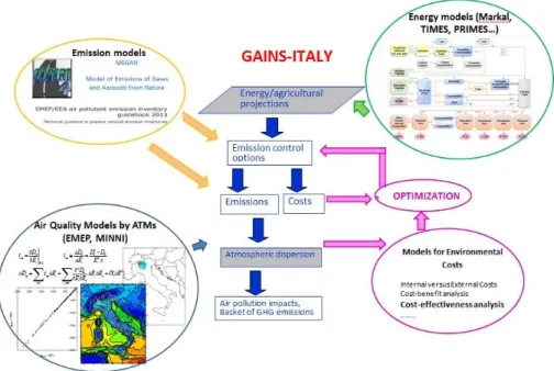
In the last years a cost-effectiveness approach has become of the utmost importance in defining several European policies on air pollution. At the beginning, almost 20 years ago, the first negotiation processes started from a common tool, the RAINS model, to establish international agreement on the main environmental issues where a flat-rate approach based on a fixed percentage of emission reductions was adopted to identify differentiated obligations for each single party. In the future years, a second generation of negotiation process has started where the cost-effectiveness analysis became the rationale to assign differential national obligations based on the carrying capacity of vulnerable ecosystems rather than a politically equitable and arbitrary emission cut (Wagner et al., 2013).
In this contest, and participating as technical experts to support the Environmental Ministry in the negotiation process, ENEA in collaboration with IIASA has decided to introduce in the MINNI project a cost-effectiveness analysis, developing an optimization tool based on the structure of the GAINS-Italy model. The tool represents the first optimization tool that acts on a national scale where all the 20 Italian Regions are considered so providing many flexibility degrees.
In the present report the methodology used in the GAINS-Italy model to find cost-effectiveness emission control strategies that address air quality issues will be described. The methodology will then be applied to two different policy scenarios in order to better explained the tool features and flexibilities. At the current state of the art, the tool affects measures that change the emission factors of one or more pollutants without affecting the activity levels (so no fuel substitutions or energy saving measures are considered).
The purpose of the present document is to introduce the tool describing firstly the MINNI project (section 2), then the main characteristics and configurations of the optimization tool and its variables (section 3 and 4). And finally in section 5, a description of the baseline and MTFR regional scenario in terms of emissions and air quality impacts as PM2.5 concentrations at the year 2030 will be presented, while in section 6 the first applications of the tool will be provided through two different policy scenarios prepared on the basis of two common approaches, the ‘absolute limit value’ and ‘gap closure’ procedure. The results of the two approaches will then be compared in terms of regional additional costs on the top of baseline scenario, sectorial regional emission reductions for each of the main pollutants and of air quality impacts.
2
MINNI PROJECT
The MINNI (National Integrated Model to support the international negotiation on atmospheric pollution) model is an ENEA project, born in 2002 and funded by MATTM (the Italian Ministry for Environment and Territory and Sea), to develop a tool able to link policy and atmospheric science, and to assess the costs of the abatement measures.
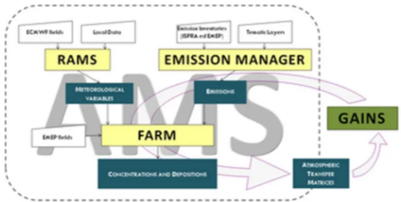
MINNI is composed by two main elements: the national AMS (Atmospheric Modeling System); and the national Integrated Assessment Model GAINS-Italy (Greenhouse Gas and Air Pollution Interactions and Synergies Model over Italy). They interact in a feedback system through ATMs (Atmospheric Transfer Matrices) and RAIL (RAINS-Atmospheric Inventory link), Figure 1.
8
Figure 1 - The MINNI model scheme (www.minni.org).
The AMS is a multi-pollutant Eulerian Atmospheric Modelling System simulating meteorological fields and computing gas and aerosol transport, diffusion and chemical reactions in atmosphere (Mircea et al., 2014). It is composed by:
- the meteorological model RAMS (Regional Atmospheric Modelling System, Cotton et al., 2003);
- the emission processor EMMA (EMission MAnager, ARIA/ARIANET, 2008);
- FARM (Flexible Air Quality Regional Model, Silibello et al., 1998, 2008; Gariazzo et al., 2007; Kukkonen et al., 2012) a three-dimensional Eulerian model that includes transport and multiphase chemistry of pollutants in the atmosphere.
EMMA generates hourly gridded emissions (Monforti and Pederzoli, 2005), used by FARM to calculate concentrations at 16 terrain level and ground depositions. EMMA and FARM produce national emissions disaggregated in a grid of 67x75 points with a resolution of 20x20 km2 or 4x4 km2.
The input emissions for EMMA are a combination of the national emission inventory (http://www.sinanet.isprambiente.it/it/sia-ispra/serie-storiche-emissioni), provided by ISPRA (Institute for Environmental Protection and Research), and the EMEP inventory (available on a 50 km resolution grid at the detail of the first level of SNAP nomenclature) for the surrounding countries. The Italian national emission inventory includes: SO2, NOx, NH3, PM, CO, VOC (Volatile
Organic Compounds), the main micro-pollutants and GHGs. Every five years starting from the year 1990, ISPRA disaggregates the inventory at a provincial level using a top-down approach based on activity-related proxy data (ISPRA, 2009; http://www.sinanet.isprambiente.it/it/sia-ispra/inventaria/disaggregazione-dellinventario-nazionale-2010), with the most relevant point sources (i.e. large energy production plants and industrial facilities). GAINS-Italy (D’Elia et al., 2009) is the MINNI component dedicated to elaborate emission scenarios to support the international evaluation and negotiation on atmospheric pollution. It is the national version of the GAINS-Europe model (Amann et al., 2011), developed by IIASA (International Institute for Applied System Analysis) and allows evaluation of impacts and costs. Starting from information on emission abatement technologies and economic scenarios of energy and productive sector, GAINS-Italy produces alternative and/or future emission scenarios, alternative air quality scenarios and abatement costs at a 5-year interval starting from 1990 to 2050.
More details about the MINNI project are available at the link http://www.minni.org/.
The AMS and GAINS-Italy are circularly related one to each other by the ATMs (Briganti et al., 2011) and RAIL. The AMS produces ATMs used by GAINS-Italy to estimate how changes in emission scenarios can affect pollutant concentrations and ground depositions. This is an approximate method, justified by administrators needs to get near real-time feedback on multiple
9
scenarios analyses, despite the heavy computational resources which the yearly runs of the complete AMS would require.
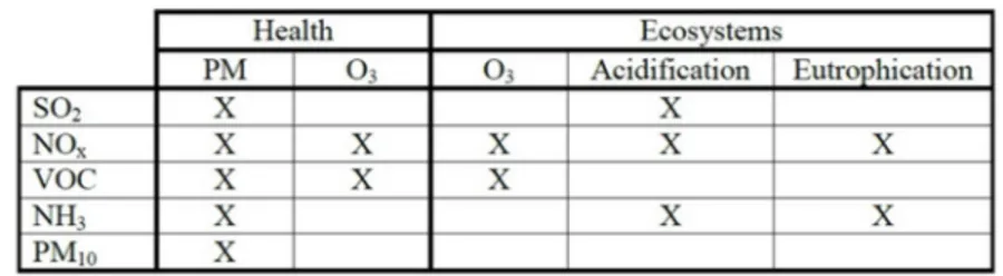
The ATMs have been computed considering the national domain at 20 km resolution by varying the following five precursors: SO2, NOx, VOC, NH3 and anthropogenic PM10. Table 1 summarizes the
influences of the previous precursors on GAINS health and vegetation impact indicators:
- NOx are involved in the ozone cycle and deposition of PM2.5, they also determine the soil
acidification and eutrophication;
- VOCs determine the ozone concentration and influence PM2.5 by the oxidation process of SO2, NOx and condensation of non-reactive VOCs;
- NH3 is involved in increasing secondary PM concentrations as ammonia salt and ground
deposition of nitrogen.
Table 1- Influence of precursors on GAINS indicators that give significant impacts on health and vegetation.
Compared to GAINS-Europe, the development of GAINS-Italy gives many advantages to the national integrated model. GAINS-Italy has a spatial resolution of 20 km, where ATMs have been calculated with the national AMS model that allows to consider orographic and meteorological regional variability.
3
THE OPTIMIZATION TOOL
The GAINS optimization module allows to identify a cost-effective policy scenario able to achieve a given environmental/health target analyzing sectors in which is more appropriate to take action to reduce emissions, technological options available for single pollutant and relative costs.
The first Italian optimization tool has been developed in collaboration with IIASA and follows the GAINS-Europe scheme.
The optimization module is external to the GAINS-Italy chain but fully integrated with the model database components (Figure 2). The software downloads data from GAINS-Italy and, after elaboration, it is possible to upload the new elaborated scenario on GAINS-Italy database. The input data downloaded from GAINS-Italy are structural and geographical information; impact-related data, such as the indicators AOT40, SOMO35, PM, NO2 and the scenario dependent data, which differ for
each baseline scenario chosen for the optimization procedure. A particular customization of the Italian version is the addition of the NO2 indicator, important to study the national road transport
emissions and to understand the its effect as PM precursor, especially for the Regions of the Po valley (MATTM, 2011).
10
Figure 2 - The GAINS-Italy model scheme.
The optimization is formulated as a Linear Programming problem, i.e., all the equations, definitions and constraints are linear in the decision variables.
Once defined an emission baseline scenario, the first step of the optimization procedure is to choose a base year and to set target values for environmental and/or human health impacts, in relation to a predefined policy target (Eq. 1).
Where hi|j,q is a function of the atmospheric transfer matrices, that links environmental constrains to
emission sources Ei,p (function of region and pollutant) and environmental impacts q (Amann et al.,
2011). The decision variable xi,f,t is the activity level in the region controlled by a specific technology
t. The optimization process follows specific rules to control the ‘permissible chain of technology’ which defines if a technology can be replaced by another and in what percentage (Wagner et al., 2013).
The second step is to minimize the total control costs (C), summing over all Regions (i), activities (f) and technologies (t), involved to reach the target (Eq. 2).
The purpose of the following paragraphs is to give a brief overlook of the main characteristics of the variables introduced in the previous equations. More details are described in Wagner et al., 2013.
3.1 Space
The GAINS-Italy model covers 20 land-based Regions (namely, the 20 Italian administrative Regions) and one sea region. Impacts are calculated on a grid with a resolution of 20 km x 20 km and then aggregated to country level. A manifold flexibility is available in the tool: the optimization could include all of the Regions, subsets of Regions, or just one Region per time.
11 3.2 Time
The GAINS-Italy model elaborates scenario in a 5-years step, starting from a base year and running into the future. The current base year for air pollutant emissions is the year 2005 whose emissions have been calibrated with the national emission inventory (D’Elia and Peschi, 2013). Currently the longest time horizon available in the model is the year 2050.
The optimization procedure is applied only to a single year period and no optimal future trajectories are provided. So the objective of the optimization is to identify cost-effective emission control strategies that meet a given set of environmental targets in that particular year.
3.3 Activities and sectors
The GAINS-Italy model considers a large combination of activities and sectors. Anyway, in the optimization process, it is considered only the case where activity data are constant. Emission reductions can so be reached by changing the application rates of control technologies, but not by changes in activity data (for example, fuel switches or energy efficiency improvements are not allowed).
3.4 Pollutants
The pollutants considered in the model are the traditional air pollutants (SO2, NOX, PM2.5, NH3 and
VOC) and the greenhouse gases (CO2, CH4, N2O, FGAS). The optimization tool focuses only on
traditional air pollutants.
3.5 Decision variables
The decision variables considered in the tool are expressed as xi,s,f,t and represent the level of the
activity f in sector s and region i controlled by technology t. Other variables have been introduced in the tool to express a technology constraint, i.e. to what extent technologies can be used beyond the baseline application rate or to what extent technologies can be replaced by better technologies. These variables are indicated with xxi,s,f,t,t’,p where t’ represents the new alternative technology. In this way,
conveniently constraining the variables xxi,s,f,t,t’,p, it is possible to allow only certain technology
transitions respect to the baseline.
3.6 Emissions
Another important variable in Eq. 1 are emissions. Emissions are calculated in GAINS-Italy model starting from the decision variable xi,s,f,t and the emission factors through the following formulation
12
where EFi,s,f,p is the unabated emission factor of pollutant p for sector s and activity f in region i.
3.7 Emission control costs
A unit cost uci,s,f,t is associated to each emission control technology. Unit costs are calculated
considering a free market so that the same technology is available to all Regions/countries at the same cost. GAINS model estimates costs for each of the 3500 emission control options considering annualized investments, fixed and variable operating costs (more details in Cofala and Syri, 1998a,b; Klimont and Winiwarter, 2011). The cost for using a technology t is then calculated as
which can be aggregated to activity-sector level as
that represents the cost to minimize in Eq. 2.
In GAINS-Italy the unit costs used for the optimization, which have been maintained equal to the GAINS-Europe values to ensure comparability between national and European results, have been verified for each pollutant, sector and fuel, for an amount of approximately 2000 curves. The costs used by GAINS-Europe for Italy have been confirmed, except for few cases where EFs have been modified and consequently also UCs (according to the shape of the EF-UC curve), or when a new curve has been defined for a typical Italian sector missing in the European version of the model (i.e. the brick sector).
3.8 Atmospheric dispersion
An integrated assessment of air pollution needs to link marginal changes in precursor emissions at the various sources to responses in impact-relevant air quality indicators (Wagner et al., 2013). The optimization task calls for computationally efficient source-receptor relationships, so simplified representations of a full air quality model through mathematically simple formulations, the ATMs, have been developed. While the GAINS-Europe relies on the Unified EMEP Eulerian model, in the GAINS-Italy model ATMs have been calculated with the AMS part of the MINNI project, as explained in paragraph 2.
ATMs are source-receptor relationships expressing the variation of concentrations/depositions in each grid point of the domain (grid of 67x75 points at 20 km spatial resolution) as a return to variations of precursor emissions for given sets of sources (in GAINS-Italy the twenty Regions). They represent the linear approximation of the response of the atmospheric system in a neighborhood of the reference conditions, as shown by the following definition (Eq. 6).
13 Where:
i, k =regional aggregates α = lattice receptors
Ei = total yearly emission from the i-th region
Cα = yearly averaged concentration over receptor α
tiα = ATM coefficients
S0 =reference scenario X = emission reduction factor
The ATMs are strictly dependent on the scenario and the meteorological condition (see tiα
coefficients), if one of that parameters changes, a new ATM calculation is required. For this reason, it is important to define meteorology-averaged ATMs, where the matrices’ coefficients are calculated using a wide case of weather conditions. The ATMs have been computed by AMS for the GAINS-Italy model considering, as reference emissions, the no climate package emission scenario for the year 2015 (‘GAINSnoCP 2015’) and, as meteorology, the years 1999, 2003, 2005, 2007 and the average-meteorological year.
For each meteorological year, the ATM coefficients have been calculated running the atmospheric modeling system 101 times (20 Regions for 5 precursors, and the reference scenario).
The GAINS model identifies cost-effective emission control scenarios based on these source-receptor relationships calculated for the average meteorological year.
3.9 Environmental targets
The aim of the GAINS optimization procedure is to identify cost-effective solutions to given environmental targets. These targets are related to the function highlighted in paragraph 3.8, i.e. PM2.5 and NO2 concentrations, change in life years (YOLL), S and N deposition and so on. Targets
can be set one by one or simultaneously and many different alternatives are possible. It is also possible to exclude from the optimization some pollutants or sectors. Targets should also be feasible, namely reachable. So it can be useful to generate the maximum technically feasible reduction scenario (MTFR, see par. 4.1) which represents the lowest achievable emission level under certain constraints. Feasible targets are so included between the baseline and MTFR scenario. Currently, the road transport sector is not optimized, because the choice of technology (EURO classes) mainly depends on normative deadlines while non-technical measures are not included until now.
Once the environmental targets have been set, minimizing the cost of control measures will identify an optimal control strategy for achieving these targets.
14
4
CONFIGURATION OF THE OPTIMIZATION
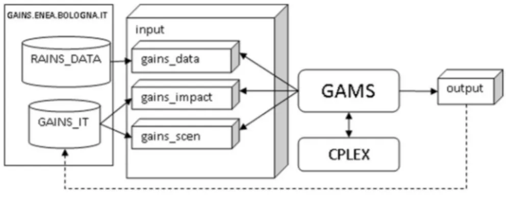
The tool is extremely flexible and each of the variables previously illustrated could be set in different ways and combinations. Moreover, the optimization algorithm is written in GAMS code that allows several personalization of the code and it is solved with the CPLEX solver. GAMS runs in a local machine and the general logic of the data flow is reported in figure 3.
Figure 3 - The optimization tool data flow.
RAINS_DATA and GAINS_IT are data schemas on the ENEA database server in Bologna. From there, data are downloaded into the local directory using SQLplus. GAMS then reads the input data and the code and builds an optimization matrix. This is then send to CPLEX which finds the optimal solution and returns it to GAMS. Finally GAMS outputs these results into .csv files and writes them into the output directory, from which they can be accessed and used for further analysis. There is also a routine to upload the control strategy back into the GAINS_IT database so that the optimized scenario is available for use through the web interface as any other model.
The GAINS optimization can be used to find cost-optimal solutions that meet predefined policy targets, such as emission ceilings, concentration ceilings, etc. The cost and feasibility of reaching such targets heavily depend on the baseline assumptions and the values of the constraints, which in turn determine the flexibility of model.
4.1 Scenario definition
Once defined the scenario and the year to optimize, the optimization tool produces four different scenarios: two Baseline, the CLE (Current LEgislation) and COB (Cost Optimal Baseline) scenarios; the MTFR (Maximum Technically Feasible Reduction); and the Policy scenarios.
The CLE scenario is the starting point of the optimization process, with no degree of freedom. Typically it reproduces the scenario showed by GAINS web-interface, keeping the activity levels and application technologies rates at the baseline level.
The COB scenario: the CLE scenario does not necessarily represent the most cost effective way to reach the baseline emission level for each source category. So in the optimization tool, it is calculated a new baseline scenario, called COB, with the most cost-effective control strategy needed to reproduce the CLE emission level for each source category.
15
The MTFR scenario represents the scenario where the sum of emissions for all air pollutants is the lowest possible using the maximum application rates of the available technologies. In this case the constraint is on the sum of emissions that has to be minimized. This is the most expensive scenario. The Policy scenario is the one where the optimization takes place and the solution reflects the choice of both targets and constraints. Policy scenario aims to be a feasible compromise between the baseline and MTFR scenario, that allows to comply with the regulation limit values at cheaper costs. The feasibility of Policy scenario depends on the Baseline scenario chosen as starting point.
4.2 The choice of the targets
The feasible optimization results are focused on Policy targets. Many different configuration could be choose in the optimization tool to reach the targets (Wagner et al., 2013), for example it is possible to choose an “absolute limit value” approach or the ‘gap closure’ approach. These are the two approaches chosen in the present work to illustrate the way the optimization tool works.
1. ‘Absolute limit value’: a uniform environmental quality criteria could be established to be achieved in all the Italian Regions. This means that there would be areas with higher polluted zones to invest more money than less polluted zones. Costs would be less but also benefits. 2. ‘Gap closure’: it is based on the idea that the feasible scenario lies between what is currently
planned (the Baseline scenario) and the MTFR scenario. The distance reduction between these two scenarios is the gap closure, that can be calculated for each pollutant and each Region. The results calculated imposing this reduction (between 0% and 100%) is the Policy scenario calculated with the ‘gap closure’ approach and policy makers could choose different gap closure depending on the ambition level they would like to reach for the different impact indicators.
The strengths of the ‘gap closure’ approach are the equality between nations which have to reduce the distance between Baseline and MTFR even if they respect the emission limits; the feasibility of the target for all the nations. The weakness is that some virtuous nations that respect air quality limits have to invest more resources to improve the already good air quality system. In establishing European policies, the ‘gap closure’ approach has been chosen to guarantee equality among community countries and to help territories with disadvantaged orography.
Considering Italian Regions, it is possible to apply the ‘gap closure’ methodology also in Italy with GAINS-Italy. In this study we show the results obtained using the ‘absolute limit value’ approach and the ‘gap closure’ approach for the Italian territory. As previously described, it is possible to optimize over more than one environmental targets and in several domains, but since the purpose of this paper is to show the methodology, the optimization has been run at year 2030 for PM2.5 on Italy considering all the 20 Regions. The absolute limit has been put equal to 20 µg/m3 at the year 2030, as required for PM2.5 concentrations by the Air Quality European Directive (EC, 2008). The gap closure percentage has been calculated with iterative runs so to reach the limit of 20 µg/m3 for all the Italian Regions. The results of these runs ended in a gap closure of 50%.
16
5
THE APPLICATION OF THE OPT TOOL TO THE WHOLE ITALIAN
TERRITORY
The development of an emission scenario with the GAINS-Italy model requires the definition of anthropogenic activity levels, both energy and non-energy, and of a control strategy with a 5-year interval for the period 1990-2050. The input energy scenario has been elaborated by ISPRA with the Markal-Italy model (Gracceva and Contaldi, 2005) and is based on the Markal software (Market Allocation), whose methodology has been developed in ETSAP (Energy Technology Systems Analysis Programme) of IEA (International Energy Agency). The energy scenario for the GAINS-Italy model used for the present work is based on the new National Energy Strategy (SEN, 2013). The first step for the preparation of a new national emission scenario is an acceptable harmonization, at a given base year, between the national emission inventory (IIR, 2013) and the GAINS-Italy emissions, estimated with a top-down approach (D’Elia and Peschi, 2013).
The baseline national anthropogenic activity level scenario was then downscaled on a regional level following a top-down approach. The regional proxies have been estimated for the base year 2005 and extended for the whole scenario and come from the regional scenario elaborated with the MINNI model for the NO2 time extension (MATTM, 2011) according to article 22 of Directive 2008/50/CE
(EC, 2008).
Once prepared the regional baseline emission scenario, the optimization tool has been run considering different policy scenarios. More information about the GAINS methodology and interactive access to input data and results are available at the following link http://www.minni.org/. All the scenario discussed in the following paragraphs can be retrieved from the GAINS-Italy online model (http://gains-it.bologna.enea.it/gains/IT/index.login?) under the Scenario group ‘Reg_OPT_Mar2014’.
5.1 The Baseline and MTFR scenario at the year 2030
The baseline scenario assumes the full implementation all over the Italian territory of the current legislation, both at a European and national level, according to the foreseen schedule. A complete description of all the national input data (energy and non-energy activity data and the control strategy) is provided in the technical report described by D’Elia and Peschi, 2013. As a first assumption all the anthropogenic activity data have been downscaled with a top-down approach while the same national control strategy has been hypothesized for all the 20 Italian Regions.
The MTFR scenario explores to what extent emissions of the various substances could be further reduced beyond what is required by current legislation, through full application of the available technical measures, without changes in the energy structures and without behavioural changes of consumers (Amann et al., 2014).
5.1.1 Emission Analysis
In the following paragraphs a brief description of the baseline and MTFR scenario by Regions will be provided for each pollutant.
Sulphur dioxide (SO2)
The implementation of the directives especially on the energy system led to a progressive SO2
17
(table 2). Most of the reductions come from power plants 84%), industry 40%) and refineries (-38%).
Table 2 - National SO2 emissions (ktons) by sector of the Baseline scenario and MTFR for the year 2030.
Sectors 2005 2010 2015 2020 2025 2030 Variation 2005- 2030 BL MTFR BL2030 MTFR2030 Power plants 148.10 60.74 25.65 25.60 23.00 23.99 11.68 -84% -92% Refineries 67.22 47.34 44.18 45.18 41.77 41.86 17.10 -38% -75% Industry (comb&proc) 104.19 66.62 62.70 65.28 62.29 62.57 39.79 -40% -62% Domestic sector 16.84 5.85 5.98 5.73 5.62 5.20 4.03 -69% -76% Fuel extraction 0.00 0.00 0.00 0.00 0.00 0.00 0.00 0% 0% Solvent use 0.00 0.00 0.00 0.00 0.00 0.00 0.00 0% 0% Road Transport 2.39 0.66 0.66 0.64 0.61 0.59 0.59 -75% -75% Non-road mobile 0.60 0.39 0.43 0.45 0.47 0.48 0.48 -19% -19% Maritime 51.86 28.47 34.55 36.51 38.30 42.66 13.63 -18% -74% Waste treatment 0.30 0.25 0.25 0.25 0.25 0.25 0.00 -18% -100% Agriculture 0.13 0.13 0.13 0.13 0.13 0.13 0.00 0% -100% Total 391.63 210.44 174.52 179.76 172.43 177.73 87.30 -55% -78%
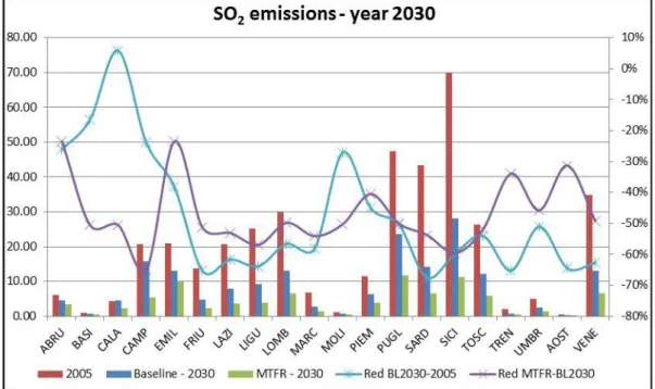
Due to the sectors involved in the emission reductions, the Regions where these reductions are observed are Lombardy, Sicily, Veneto, Puglia and Sardinia whose emission reductions vary around 60-65% (figure 4).
Figure 4 - SO2 emissions (ktons) by Regions at the year 2005 (red bar) and at the year 2030 for the Baseline (blue bar)
and MTFR (green bar) scenario. The pale-blue line shows the emission variation (in %) from the year 2005 to the year 2030; while the purple line the variation at the year 2030 between the Baseline and MTFR scenario.
The full implementation of the available technical emission control measures (MTFR scenario) could bring SO2 emissions in 2030 78% down compared to 2005 (table 2).
18
Nitrogen oxides (NOX)
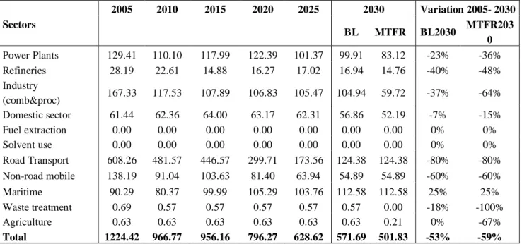
The implementation of current legislation could lead also for NOX to a significant reduction (-53% in
2030 respect to 2005) that comes especially from the transport sector, both road (-80%) and non-road (-60%), and industry (-37%). In the maritime sector an emission increase is observed (table 3).
Table 3- National NOx emissions (ktons) by sector of the Baseline scenario and MTFR for the year 2030.
Sectors 2005 2010 2015 2020 2025 2030 Variation 2005- 2030 BL MTFR BL2030 MTFR203 0 Power Plants 129.41 110.10 117.99 122.39 101.37 99.91 83.12 -23% -36% Refineries 28.19 22.61 14.88 16.27 17.02 16.94 14.76 -40% -48% Industry (comb&proc) 167.33 117.53 107.89 106.83 105.47 104.94 59.72 -37% -64% Domestic sector 61.44 62.36 64.00 63.17 62.31 56.86 52.19 -7% -15% Fuel extraction 0.00 0.00 0.00 0.00 0.00 0.00 0.00 0% 0% Solvent use 0.00 0.00 0.00 0.00 0.00 0.00 0.00 0% 0% Road Transport 608.26 481.57 446.57 299.71 173.56 124.38 124.38 -80% -80% Non-road mobile 138.19 91.04 103.63 81.40 63.94 54.89 54.89 -60% -60% Maritime 90.29 80.37 99.99 105.29 103.76 112.58 112.58 25% 25% Waste treatment 0.69 0.57 0.57 0.57 0.57 0.57 0.00 -18% -100% Agriculture 0.63 0.63 0.63 0.63 0.63 0.63 0.21 0% -67% Total 1224.42 966.77 956.16 796.27 628.62 571.69 501.83 -53% -59%
A very high reduction in NOX emissions is expected in Lombardy Region followed by Emilia
Romagna, Lazio and Veneto (figure 5).
Figure 5 - NOx emissions (ktons) by Regions at the year 2005 (red bar) and at the year 2030 for the Baseline (blue bar)
and MTFR (green bar) scenario. The pale-blue line shows the emission variation (in %) from the year 2005 to the year 2030; while the purple line the variation at the year 2030 between the Baseline and MTFR scenario.
19
Full implementation of additional measures in stationary sources could lead to further reductions, but not so high as observed for SO2, because the transport sector will remain also in the future the most
polluting sector. Moreover, in the most emitting NOX Regions, the reductions observed in the MTFR
scenario are limited (figure 5).
Fine particulate matter (PM2.5)
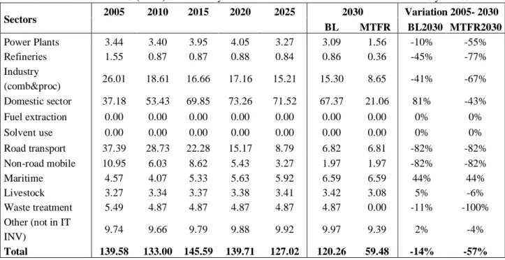
The two main emitting sectors for PM2.5 at the year 2005 are the road transport and domestic sectors that account more than 50% of total emissions. While for the transport sector a huge emission reduction is foreseen at the year 2030 (-82%) due to the progressive replacement of gasoline car fleet with diesel and to the introduction of diesel particle filters, a same increase (+81%) is foreseen for the domestic sector due to a heavily diffusion of fuelwood in small stationary sources that will lead the domestic sector to be the main emitting sector with a contribution of 56% to total PM2.5 emissions (table 4). This means that a more limited emission reduction (-14%) is estimated at the year 2030 respect to 2005.
Table 4 - National PM2.5 (ktons) emissions by sector of the Baseline scenario and MTFR for the year 2030.
Sectors 2005 2010 2015 2020 2025 2030 Variation 2005- 2030 BL MTFR BL2030 MTFR2030 Power Plants 3.44 3.40 3.95 4.05 3.27 3.09 1.56 -10% -55% Refineries 1.55 0.87 0.87 0.88 0.84 0.86 0.36 -45% -77% Industry (comb&proc) 26.01 18.61 16.66 17.16 15.21 15.30 8.65 -41% -67% Domestic sector 37.18 53.43 69.85 73.26 71.52 67.37 21.06 81% -43% Fuel extraction 0.00 0.00 0.00 0.00 0.00 0.00 0.00 0% 0% Solvent use 0.00 0.00 0.00 0.00 0.00 0.00 0.00 0% 0% Road transport 37.39 28.73 22.28 15.17 8.79 6.82 6.81 -82% -82% Non-road mobile 10.95 6.03 8.62 5.43 3.27 1.97 1.97 -82% -82% Maritime 4.57 4.07 5.33 5.63 5.92 6.59 6.59 44% 44% Livestock 3.27 3.34 3.37 3.38 3.41 3.42 3.08 5% -6% Waste treatment 5.49 4.87 4.87 4.87 4.87 4.87 0.00 -11% -100% Other (not in IT INV) 9.74 9.66 9.79 9.88 9.92 9.97 9.39 2% -4% Total 139.58 133.00 145.59 139.71 127.02 120.26 59.48 -14% -57%
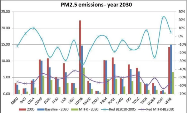
The regional emission baseline variation at the year 2030 respect to the year 2005 is extremely irregular (figure 6) and not always a reduction is foreseen. Being the domestic sector a high potential sector to reduce emissions, the full implementation of additional measures could bring PM2.5 emissions in 2030 57% down compared to 2005 (table 4).
20
Figure 6 - PM2.5 emissions (ktons) by Regions at the year 2005 (red bar) and at the year 2030 for the Baseline (blue bar) and MTFR (green bar) scenario. The pale-blue line shows the emission variation (in %) from the year 2005 to the year
2030; while the purple line the variation at the year 2030 between the Baseline and MTFR scenario.
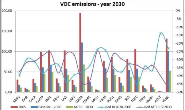
Volatile organic compounds (VOC)
Road transport and solvent use, both domestic and industrial, are the main emitting sectors (respectively 32% and 39% of total VOC emissions at the year 2005) and the implementation of current legislation could lead to an emission reduction of 35% at the year 2030 (table 5). As for PM2.5, the high fuelwood diffusion will influence VOC emission reductions, and an increase of 78% is foreseen in the domestic sector in the baseline scenario at the year 2030.
Table 5 - National VOC emissions (ktons) by sector of the Baseline scenario and MTFR for the year 2030.
Sectors 2005 2010 2015 2020 2025 2030 Variation 2005- 2030 BL MTFR BL2030 MTFR2030 Refineries 23.84 18.16 20.39 19.91 20.07 21.25 14.04 -11% -41% Domestic sector 67.13 91.77 120.64 128.12 126.37 119.36 67.26 78% 0% Other stationary sources 66.99 67.96 69.73 70.92 71.20 75.71 54.34 13% -19% Domestic solvent use 218.05 172.53 172.16 170.54 169.94 171.02 83.23 -22% -62% Industrial solvent use 262.10 221.50 212.38 205.77 204.02 201.96 88.89 -23% -66% Fuel extraction 60.41 53.38 52.59 51.89 51.35 51.48 50.34 -15% -17% Road transport 396.07 243.97 163.98 116.08 83.41 60.87 60.87 -85% -85% Non-road mobile 132.79 104.54 109.82 103.43 100.20 98.65 98.64 -26% -26% Waste treatment 12.03 10.46 8.86 6.22 4.69 4.69 3.74 -61% -69% Total 1239.41 984.27 930.55 872.88 831.25 804.99 521.34 -35% -58%
21
Also for VOC, the regional emission reduction in the baseline scenario is extremely irregular (figure 7), while the potential for further emission reductions is high and could bring VOC emissions in 2030 58% down compared to 2005 due to the still high possibility to reduce solvent emissions.
Figure 7 - VOC emissions (ktons) by Regions at the year 2005 (red bar) and at the year 2030 for the Baseline (blue bar) and MTFR (green bar) scenario. The pale-blue line shows the emission variation (in %) from the year 2005 to the year
2030; while the purple line the variation at the year 2030 between the Baseline and MTFR scenario.
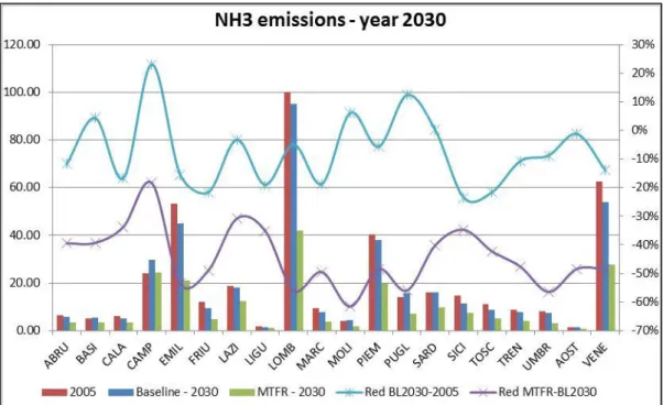
Ammonia (NH3)
Agriculture represents the main ammonia emitting sector (almost 92% of total NH3 emissions at
2005) and due to the absence of legislation for cattle and fertilizer use, slight reductions are expected up to 2030 (-7%). This means that there is a very high emission potential reduction and if the available measures were applied a 51% emission reduction could be expected (table 6).
Table 6 -National NH3 emissions (ktons) by sector of the Baseline scenario and MTFR for the year 2030.
Sectors 2005 2010 2015 2020 2025 2030 Variation 2005- 2030 BL MTFR BL2030 MTFR2030 Cattle 185.31 173.63 175.16 169.17 167.89 165.49 92.83 -11% -50% Pigs 49.30 48.27 49.00 49.33 49.69 50.19 15.59 2% -68% Poultry 37.86 38.64 38.87 39.17 39.77 39.99 16.95 6% -55% Sheep 11.60 11.57 11.47 11.63 11.74 11.82 9.17 2% -21% Urea fertilizer 59.24 39.79 47.54 51.39 51.39 51.39 2.91 -13% -95% Other N fertilizer 17.25 10.53 11.23 12.39 12.39 12.39 12.39 -28% -28% Other livestock 24.17 30.66 31.82 35.03 37.97 40.92 40.90 69% 69% Waste treatment 10.04 9.49 7.31 5.03 3.71 3.71 3.44 -63% -66% Transport 17.29 10.72 7.31 6.37 6.06 6.25 6.24 -64% -64% Stationary sources 6.42 4.25 4.82 5.38 5.53 5.68 5.12 -12% -20% Total 418.48 377.55 384.53 384.89 386.14 387.83 205.54 -7% -51%
22
Ammonia emissions occur especially in the Po Valley, so for the Regions that stand on that area a very high emission reduction could be reached (figure 8).
Figure 8 - NH3 emissions (ktons) by Regions at the year 2005 (red bar) and at the year 2030 for the Baseline (blue bar)
and MTFR (green bar) scenario. The pale-blue line shows the emission variation (in %) from the year 2005 to the year 2030; while the purple line the variation at the year 2030 between the Baseline and MTFR scenario.
5.1.2 Air Quality Impacts
The starting point for the cost-effectiveness analysis is the review of the baseline air quality impact indicators and the outline of the scope for further reduction that could be achieved through the implementation of additional measures of the MTFR scenario. The air quality indicator that would be examined in the present work is the attainment of the annual air quality limit value for PM2.5 concentrations at the year 2030.
The PM2.5 annual air quality limit value required by the Air Quality Directive at the year 2030 is 20 mg/m3
. The GAINS-Italy model, as highlighted in paragraph 2, allows to calculate PM2.5 concentration maps for the whole Italian territory at a resolution of 20 km for 5 meteorological years. The meteorology considered for the cost-effectiveness analysis is the average year. So under these conditions and although the improvements from the implementation of the current air legislation, the PM2.5 annual limit value in the baseline 2030 scenario will not be met in different areas of the Italian territory (figure 9).
Exceedances in the baseline scenario are observed in the Po Valley, in the area of Milan and Naples (figure 9, left).
Figure 9 shows also that the 2030 MTFR scenario allows to attain the PM2.5 annual limit value (the maximum concentration is 16 mg/m3
) but at a very high cost. So an optimization analysis becomes of the utmost importance to reach the target at a sustainable cost.
23
Figure 9 – Annual PM2.5 concentration at the year 2030 in the Baseline (left) and MTFR (right) scenario.
6
THE POLICY SCENARIO AT THE YEAR 2030
To show the importance of the choice of the approach in deciding how to reach the target, two different approaches have been followed with the common purpose to attain the PM2.5 annual limit value of 20 mg/m3
at the year 2030.
The first policy scenario has been obtained following the same European method of the gap closure approach (Amann et al., 2014). The choice of the gap is crucial in order to balance costs and efforts. Several runs of the optimization tool have been conducted for a series of increasingly stringent gap closure target for PM2.5 concentration. The gap chosen represents the minimum gap that allows to attain the limit of 20 mg/m3
at the year 2030 all over the Italian territory and it turns out to be a gap of 50%. The second policy scenario has been elaborated imposing the absolute value of 20 mg/m3
at the year 2030 for all the Italian domain. So both the policy scenarios have as common target the attainment of the PM2.5 limit value of 20 mg/m3
at the year 2030.
In the following, the differences between the two policy scenarios will be shown. 6.1 Emission control costs
The results in terms of additional costs by Regions (on top of the baseline scenario) are shown in Figure 10.
The gap closure approach implies that all Regions must reduce the gap between the baseline and the MTFR scenario notwithstanding the already attainment of the PM2.5 limit value in the baseline. As a consequence all Regions have to invest money in reducing PM2.5 concentrations while in the policy scenario ‘absolute limit value’ only Regions in non-compliance have to reduce emissions and PM2.5 concentrations. The ‘gap closure’ scenario requires an additional total cost over the baseline scenario of 1494 M€ (figure 10) while the ‘absolute limit value’ policy scenario has additional costs of 479 M€.
24
Figure 10 – Additional costs (in M€) that each Region has to support in order to reduce PM2.5 concentration in the two POLICY scenarios – 50% gap closure (green bar) and Absolute Value of 20 mg/m3
(blue bar) – and in the MTFR scenario (red bar) at the year 2030.
6.2 Emission reductions
The differences are evident not only in terms of costs but of course in terms of emission reductions and PM2.5 concentrations both as Regions involved and amount of sectorial emission reductions as the following figures show.
For example, for NOX emissions in the Lombardy Region in the absolute policy scenario, 1.6 ktons
could be reduced instead of 5 ktons of the gap closure and in the first case it is sufficient to reduce emissions from stationary engines. More evident are the differences in NH3 emission reductions
where to reduce PM2.5 concentration, the Lombardy Region should, for example, reduce emissions of almost 20 ktons in the gap closure scenario while a reduction of 5 ktons is foreseen in the absolute one.
25
Figure 11 – Comparison, in terms of SO2 emission reduction (ktons/y) at the year 2030, between the policy 50 gap
closure (left) and the policy absolute value (right) scenarios.
Figure 12 – Comparison, in terms of NOX emission reduction (konst/y) at the year 2030, between the policy 50 gap
closure (left) and the policy absolute value (right) scenarios.
Figure 13 – Comparison, in terms of PM2.5 emission reduction (ktons/y) at the year 2030, between the policy 50 gap closure (left) and the policy absolute value (right) scenarios.
26
Figure 14 – Comparison, in terms of VOC emission reduction (ktons/y) at the year 2030, between the policy 50 gap closure (left) and the policy absolute value (right) scenarios.
Figure 15 – Comparison, in terms of NH3 emission reduction (ktons/y) at the year 2030, between the policy 50 gap
closure (left) and the policy absolute value (right) scenarios.
6.3 Air quality impact on PM2.5 concentrations
As shown in figure 16, both the policy scenarios allow to reach the target value of 20 mg/m3
but in the gap closure a higher effort is requested to the Regions both in terms of costs and emission reductions than the absolute one. On the other hand, a higher PM2.5 concentration reduction would let higher benefits.
In the ‘absolute limit value’ policy scenario the highest polluted areas have to invest more money into clean-up, while there would be no incentives for improvements that are possible in less polluted areas. Costs are less, with less emission reductions and less benefits than the ‘gap closure’ policy scenario where each Region participates to the overall effort so benefits of a policy are somehow shared proportionally by all affected areas. The choice of the best approach depends of course on policy makers requirements or wishes and different approaches could be in turn adapted to the purpose the decision makers would like to reach.
27
Figure 16 – Annual PM2.5 concentration (in mg/m3
) at the year 2030 with a spatial resolution of 20 km in the 50% ‘gap
closure’ policy scenario (left) and in the ‘absolute limit value’ policy scenario (on the right).
6.4 The upload of the policy scenarios in the GAINS-ITALY model
As highlighted in paragraph 4 and shown in figure 2, all the policy scenarios calculated by the optimization tool can then be uploaded in the GAINS-Italy model so that the results can be shown through the web interface and made transparent and public. Moreover, some of the functions of the GAINS-Italy model can be exploited to analyse the results in a different way.
It has been previously underlined that the tool runs considering the average meteorological year while the ATMs have been calculated for five meteorological years (1999, 2003, 2005, 2007 and the average year). Uploading the policy scenarios in the GAINS-Italy model, it could so be also possible to show the results in terms of impact considering different meteorological years.
The following figure shows how the PM2.5 concentrations at year 2030 of the ‘absolute limit value’ scenario, elaborated by the GAINS-Italy model, change if the meteorological year 2005 is considered instead of the average meteorological year.
From figure 17, it emerges that the limit of 20 mg/m3
would not be attained in the area of Milan and Naples with the meteorological year 2005.
28
Figure 17 – Annual PM2.5 concentration (in mg/m3
) at the year 2030 with a spatial resolution of 20 km in the ‘absolute
limit value’ policy scenario calculated by the GAINS-Italy model with the average meteorological year (on the left) and
with the 2005 meteorological year (on the right).
7
CONCLUSIONS
In this report the main characteristics of the new Italian optimization module for the GAINS-Italy model have been summarized, with a particular emphasis on cost-effective control strategies that address environmental impact indicators related to air pollution.
In the first part of the present report, the various formal aspects of the optimization, including the dimension of the solution space, nature and use of decision variables and their relation to relevant functions, such as costs, emissions and environmental impact indicators, have been presented. Then the main standard optimization configurations used to calculate commonly scenarios have been illustrated. While in the second part of the report, the first results of the application of the optimization tool to all the 20 Italian Regions have been presented.
The tool has been applied for the first time following two different approaches with the common purpose to attain the PM2.5 annual limit value of 20 mg/m3
at the year 2030.
The first policy scenario has been obtained following the ‘gap closure’ procedure that allows to set feasible targets and that respects at the same time the need to distribute equally environmental benefits among Regions. The second policy scenario is based on the ‘absolute limit value’ approach that establishes a uniform environmental quality criteria for all the Regions. In terms of additional costs over the baseline scenario, the ‘gap closure’ scenario requires 1494 M€ while the ‘absolute limit value’ policy scenario has additional costs of 479 M€. Also emission reductions vary differently among Regions for each pollutant but of course, the benefits in terms of air quality impact reductions are much lower in the absolute approach. The choice of the best approach depends on policy makers requirements or wishes and different approaches could be in turn adapted to the purpose the decision makers would like to reach.
Anyway, the tool can be used to aid policy makers to contemplate policy options with the required flexibility, without losing sight of cost-effectiveness considerations.
29
BIBLIOGRAPHY
Amann, M., Bertok, I., Borken-Kleefeld, J., Cofala, J., Heyes, C., Höglund-Isaksson, L., Klimont, Z., Nguyen, B., Posch, M., Rafaj, P., Sandler, R., Schöpp, W., Wagner, F., Winiwarter, W., 2011. Cost-effective control of air quality and greenhouse gases in Europe: Modeling and policy applications. Environmental Modelling & Software 26, 1489-1501.
Amann, M., Borken-Kleefeld, J., Cofala, J., Hettelingh, J-P., Heyes, C., Hoglund, L., Holland, M., Kiesewetter, G., Klimont, Z., Rafaj, P., Posch, M., Sander, R., Schöpp, W., Wagner, F., Winiwarter, W., 2014. The Final Policy Scenarios of the EU Clean Air Policy Package. TSAP Report #11, Version 1.0, International Institute for Applied Systems Analysis (IIASA), Laxenburg, Austria, February 2014.
ARIA/ARIANET, 2008. EMMA (EMGR/make) User Manual, R2008.99. Arianet, Milano, Italy.
Briganti, G., Calori, G., Cappelletti, A., Ciancarella, L., D’Isidoro, M., Finardi, S., Vitali, L., 2011. Determination of multi-year atmospheric transfer matrices for GAINS-Italy model. High Performance Computing on CRESCO infrastructure: research activities and results 2010-2011 (Report Cresco), 45-51.
Cofala, J. & Syri, S. (1998a), Nitrogen oxides emissions, abatement technologies and related costs for europe in the RAINS model database, Technical report, International Institute for Applied Systems Analysis (IIASA), Laxenburg, Austria.
Cofala, J. & Syri, S. (1998b), Sulfur emissions, abatement technologies and related costs for europe in the RAINS model database, Technical report, International Institute for Applied Systems Analysis (IIASA), Laxenburg, Austria.
Cotton, W.R., Pielke, R.A., Walko, R.L., Liston, G.E., Tremback, C.J., Jiang, H., et al., 2003. RAMS 2001: current status and future directions. Meteorol. Atmos. Phys. 82, 5-29.
D’Elia, I., Bencardino, M., Ciancarella, L., Contaldi, M., Vialetto, G., 2009. Technical and Non-technical measures for air pollution emission reduction: The integrated assessment of the Regional Air Quality Management Plans through the Italian national model. Atmospheric Environment, 43, 6182-6189.
D’Elia, I., Peschi, E., 2013. Lo scenario emissivo nazionale nella negoziazione internazionale. ENEA Technical Report, RT/2013/10/ENEA (in Italian).
EC, 2008. Directive 2008/50/EC of the European Parliament and of the Council of 21 May 2008 on ambient air quality and a cleaner air for Europe. EC Official Journal L 152 of 11.06.2008.
Gariazzo, C., Silibello, C., Finardi, S., Radice, P., Piersanti, A., Calori, G., et al., 2007. A gas/aerosol air pollutants study over the urban area of Rome using a comprehensive chemical transport model. Atmos. Environ. 41, 7286-7303.
Gracceva, F., Contaldi, M., 2005. Italian Energy Scenarios – Evaluation of Energy Policy Measures. ENEA, Rome (in Italian).
Klimont, Z. &Winiwarter,W. (2011), Integrated ammonia abatement - modelling of emission control potentials and costs in GAINS, IIASA Interim Report IR-11-027, International Institute for Applied Systems Analysis (IIASA), Laxenburg, Austria.
Kukkonen, J., Olsson, T., Schultz, D.M., Baklanov, A., Klein, T., Miranda, et al., 2012. A review of operational, regional-scale, 648 chemical weather forecasting models in Europe. Atmos. Chem. Phys. 12, 187.
30
MATTM, 2011.
http___circa.europa.eu_Public_irc_env_ambient_library_l=_notifications_extensions_it_notification_20092011_official_ notification__doc_nazionali_pianificazionepdf__EN_1
Mircea, M., Ciancarella, L., Briganti, G., Calori, G., Cappelletti, A., Cionni, I., Costa, M., Cremona, G., D’Isidoro, M., Finardi, S., Pace, G., Piersanti, A., Righini, G., Silibello, C., Vitali, L., Zanini, G., 2014. Assessment of the AMS-MINNI system capabilities to simulate air quality over Italy for the calendar year 2005. Atmospheric Environment, 84, 178-188.
Monforti, F., Pederzoli, A., 2005. THOSCANE: a tool to detail CORINAIR emission inventories. Environ. Model. Softw. 20, 505-508.
SEN, 2013. The new National Energy Strategy.
http://www.mise.gov.it/images/stories/documenti/SEN_EN_marzo2013.pdf
Silibello, C., Calori, G., Brusasca, G., Catenacci, G., Finzi, G., 1998. Application of a photochemical grid model to Milan metropolitan area. Atmos. Environ. 32 (11), 2025-2038.
Silibello, C., Calori, G., Brusasca, G., Giudici, A., Angelino, E., Fossati, G., et al., 2008. Modelling of PM10 concentrations over Milano urban area using two aerosol modules. Environ. Model. Softw. 23, 333-343.
Wagner, F., Amann, M., Wolfgang S., 2007. The GAINS Optimization Module as of February 2007. IIASA Internal Report, IR-07-004.
Wagner, F., Chris H., Zbigniew, K., Wolfgang S., 2013. The GAINS optimzation module: Identifying cost-effective measures for improving air quality and short-term climate forcing. IIASA Internal Report, IR-13-001.
Edito dall’
Servizio Comunicazione
Lungotevere Thaon di Revel, 76 - 00196 Roma www.enea.it
Stampa: Tecnografico ENEA - CR Frascati Pervenuto il 5.6.2014