ESTI
MATI
NG
THE
C-
FACTOR
OF
USLE/RUSLE
BY
MEANS
OF
NDVI
TI
ME-
SERI
ES
I
N
SOUTHERN
LATI
UM
An i
mproved correl
ati
on model
S. GRAUSO
Territorialand Production Systems Sustainability Department Division Models and Technologies for Risks reduction Laboratory of Seismic Engineering and Prevention of NaturalRisks Casaccia Research Centre
V
V. VERRUBBI, A. PELOSO
Territorialand Production Systems Sustainability Department Division Models and Technologies for Risks reduction Laboratory of Seismic Engineering and Prevention of NaturalRisks FrascatiResearch Centre
M. SCIORTINO
Territorialand Production Systems Sustainability Department Division Models and Technologies for Risks reduction Laboratory of Climate Modeling
Casaccia Research Centre
A. ZINI
Studies and Strategies Unit Studies and Strategies Unit FrascatiResearch Centre
RT/2018/9/ENEA
ITALIAN NATIONAL AGENCY FOR NEW TECHNOLOGIES, ENERGY AND SUSTAINABLE ECONOMIC DEVELOPMENT
S. GRAUSO
Territorial and Production Systems Sustainability Department Division Models and Technologies for Risks reduction Laboratory of Seismic Engineering and Prevention of Natural Risks Casaccia Research Centre
V. VERRUBBI, A. PELOSO
Territorial and Production Systems Sustainability Department Division Models and Technologies for Risks reduction Laboratory of Seismic Engineering and Prevention of Natural Risks Frascati Research Centre
ESTIMATING THE C-FACTOR OF USLE/RUSLE BY
MEANS OF NDVI TIME-SERIES IN SOUTHERN LATIUM
An improved correlation model
M. SCIORTINOTerritorial and Production Systems Sustainability Department Division Models and Technologies for Risks reduction Laboratory of Climate Modeling
Casaccia Research Centre
A. ZINI
Studies and Strategies Unit Frascati Research Centre
RT/2018/9/ENEA
ITALIAN NATIONAL AGENCY FOR NEW TECHNOLOGIES, ENERGY AND SUSTAINABLE ECONOMIC DEVELOPMENT
I rapporti tecnici sono scaricabili in formato pdf dal sito web ENEA alla pagina www.enea.it I contenuti tecnico-scientifici dei rapporti tecnici dell’ENEA rispecchiano
l’opinione degli autori e non necessariamente quella dell’Agenzia
The technical and scientific contents of these reports express the opinion of the authors but not necessarily the opinion of ENEA.
ESTIMATING THE C-FACTOR OF USLE/RUSLE BY MEANS OF NDVI TIME-SERIES IN SOUTHERN LATIUM
An improved correlation model
S. Grauso, V. Verrubbi, A. Peloso, A. Zini, M. Sciortino Riassunto
Il presente lavoro, incentrato sull'area del Lazio meridionale comprendente le province di Latina e Fro-sinone, ha avuto come oggetto la ricerca di un modello di correlazione per la previsione del fattore di gestione e copertura del suolo (fattore C del modello USLE/RUSLE) a partire da dati satellitari sinte-tizzati nell'indice di vegetazione NDVI (Normalized Difference Vegetation Index). A tal fine sono state utilizzate le serie di immagini, con risoluzione spaziale di 250 m, raccolte nel periodo 2001-2016 dalla piattaforma MODIS (Moderate Resolution Imaging Spectroradiometer). In assenza di dati osservativi diretti, relativamente alle condizioni di copertura del suolo nell'area investigata, sono stati utilizzati i valori riportati nella carta del fattore C dell'Unione Europea, con risoluzione di 100 m, realizzata dal JRC (Joint Research Center) sulla base di dataset pan-europei (CORINE Land Cover, NUTS, MERIS). L'analisi di regressione ha evidenziato come un semplice modello lineare non è in grado di prevedere con adeguata precisione i valori del fattore C relativi ai diversi tipi di coperture ed usi del suolo, in funzione dell'NDVI. Diversamente, una funzione logistica sigmoide consente una maggiore precisione nel riprodurre le relazioni tra le due variabili (R2= 0.989, RMSE = 0.015). Il confronto tra la distribuzione
dei valori del fattore C ottenuti nell'area di studio tramite la suddetta funzione e quelli riportati nella mappa del JRC ha evidenziato un buon accordo nonostante alcune incertezze, soprattutto nelle aree soggette a seminativi, dovute alle diverse tecniche utilizzate nei due casi. Il maggior beneficio deri-vante dall'applicazione del modello di correlazione qui proposto consiste nella possibilità di aggiornare la mappa, e di conseguenza i valori di C, in funzione dei dati spettrali raccolti negli anni successivi, anche con riferimento a diverse scansioni temporali (annuale, stagionale, mensile).
Parole chiave: telerilevamento, NDVI, uso del suolo, RUSLE, analisi di regressione.
Abstract
A correlation analysis between mean Normalized Difference Vegetation Index (NDVI), derived from 250m-resolution MODIS-imagery time-series (2001-2016), and mean long-term cover management (C-factor) data from the available 100m-resolution raster map, provided by the EU-JRC at the European scale, is here presented. The aim was to find out a regression model helpful to easily estimate the land cover management factor of the RUSLE, for future applications at different timescales and sub-regional level, by using the remotely sensed vegetation index as predictor. The regression analysis suggested that a sigmoid logistic function can fit well with the relationship between the two variables (R-square = 0.989, RMSE = 0.015). The model function was employed to draw the long-term C-factor map of southern Latium test-area (central Italy) which resulted in good agreement with the EU map. Some uncertainties were likely due to differences in raster resolution and technique adopted in the two approaches. Examples of simulations at annual and seasonal timescale are also provided, proving the versatility of the proposed model to estimate the C-factor at differently refined timescales and to easily draw updated maps basing on the availability of NDVI data-series.
Preface
1. Introduction
2. Background framework 3. Test-area description 4. NDVI Data analysis
5. Model analysis and application 6. Conclusions Acknowledgements References 6 7 8 11 13 17 25 25 26 INDEX
6
PREFACE
This report ends a study started in 2013 concerning the soil erosion risk assessment of Southern Latium. A first part was published in the ENEA Technical Reports series in 2015 (RT/2015/22/ENEA). As already specified in the former report, the present study was inspired by the wide investigations that ENEA and some Dutch pedologists have being carried out in the area during the 80s, which allowed to gather a considerable database concerning the physical and chemical characteristics of soils.
This second part, as well as the first part of the study, did not benefit from grants, which is why no field data check was possible which would have allowed a suitable validation of the results. The expectation is that the whole work presented could be useful to the management of soil resource both in Latium and in the other Italian Regions.
PREMESSA
Con il presente Rapporto si conclude uno studio avviato nel 2013 riguardante il rischio di erosione del suolo nel Lazio meridionale, di cui una prima parte è stata pubblicata dagli stessi autori nella serie dei Rapporti Tecnici (RT) ENEA nel 2015 (RT/2015/22/ENEA). Come è stato precisato nel primo Rapporto, lo studio ha preso le mosse dalle vaste indagini condotte in quest'area dall'ENEA e da alcuni pedologi olandesi, nel corso degli anni '80, che hanno consentito di raccogliere una consistente base di dati relativi alle caratteristiche chimico-fisiche dei suoli.
Anche questa seconda parte non ha goduto di supporti finanziari, per cui, anche in questo caso, non è stato possibile raccogliere dati osservativi sul campo che avrebbero consentito una piena validazione dei risultati. L'auspicio è che il lavoro condotto, nella sua globalità, possa dimostrarsi utile per la gestione e la guida delle politiche regionali riguardanti la risorsa suolo non solo del Lazio, ma anche delle altre regioni italiane.
7
1. Introduction
The Universal Soil Loss Equation USLE (Wischmeier & Smith 1978) and its revised version RUSLE (Renard et al. 1991, 1996) is one of the most widely used empirical models in soil erosion assessment. The model estimates the long-term yearly rate of soil loss in mass units per unit area by the product of six major parameters representing the main natural agent (rainfall erosivity R) and the soil predisposing factors to erosion (soil erodibility K and terrain morphology given by the product of slope lenght L and slope steepness S) combined with land use effects (soil cover management C and supporting practices P) :
A=R∙K∙LS∙C∙P (1)
Although the USLE was initially calibrated for single plots on gentle slopes in agricultural fields, based on long series of observations in eastern USA, this empirical parametric model have been applied worldwide on various areal extents. Soil erosion maps at continental and national level using the RUSLE approach have been drawn in latest years in Europe (van Camp et al. 2004, Panagos et al. 2015a). In Italy, applications have been performed at national and regional scale (van der Knijff et al. 1999; Grimm et al. 2003; Guermandi et al. 2006; Rusco et al. 2007; ARPAV 2008; Bagarello et al. 2008; Terranova et al. 2009; Binetti 2011; Piccini et al. 2012; Giovannozzi et al. 2013).
The main question in using the USLE/RUSLE model at regional or sub-regional scale concerns the use of simplified estimates and interpolation techniques for the spatial analysis of model parameters. This is the case for rainfall erosivity and soil erodibility whose estimate is made possible by means of different techniques and methodologies which have been proposed to solve the limitations due to the geographic area scale. Correlation formulae and spatial interpolation algorithms have been developed to allow the calculation and mapping of these variables basing on available datasets, e.g., published soil texture data and rainfall amounts at different time-steps (yearly, monthly and daily). Moreover, the variability and the uncertainty in these estimates have been discussed by various authors (Römkens et al. 1986; Young et al. 1990; Borselli 1993; Torri et al 1997; Wang et al. 2001; Lark et al 2006; Salvador Sanchis et al. 2008; Angulo-Martínez 2009; Braunović et al. 2010; Buttafuoco et al 2011; Borselli et al. 2012; Jamshidi et al 2014).
Simplified solutions have been also provided for the calculation of the topographic factor (LS). This can be easily computed by means of programs running in GIS environment that are based on digital elevation models with suitable terrain resolution (Moore and Wilson 1992; Hickey et al 1994; Desmet and Govers 1996; Mitasova et al 1996; Hickey 2000; Van Remortel et al 2001, 2004).
With regard to the anthropic variables of the RUSLE, the supporting practices factor (P) has been generally neglected so far at the scales cited above, given its very local value and the difficulty to assess it for large areas. Recently, a study attempted to model the P-factor at the European Union scale by taking into account the Common Agricultural Policy implementation on the basis of field observations carried out in each of the member states (Panagos et al., 2015b). The study provided a list of the average estimated P-factor for each EU Country and two maps showing its distribution at the Union and regional level.
Lastly, the quick and simplified estimate of the cover management factor (C) remains an open question. C is a rather complex factor to evaluate in order to parameterize the effect of actual
8
land cover and management on soil erosion. It is function of different sub-factors, such as: previous land-use, canopy-cover, surface cover, surface roughness, and soil moisture (Renard et al., 1996). These factors should be estimated for each time period of the year over which the single sub-factors is assumed to be constant, taking into account the seasonal variations due to crop rotation or other natural effects (climate variability, plant health conditions etc.). However, this procedure is rather onerous when applied on large areal extents. For this reason, an alternative technique was introduced by exploiting the ability of remote sensing technology to detect vegetation and its condition. This capability can help to minimize the field work and allows to estimate the C-factor with a spatial detail comparable to the geometric resolution of remotely sensed imagery which, in last generation sensors, can achieve a detail smaller than 1 m on ground. The most well-known and used index for this purpose is the Normalized Difference Vegetation Index (NDVI) obtained from the near-infrared and red spectral bands of the solar radiation:
(2)
The NDVI is an indicator of plant reflectance in the red and near-infrared spectral region helpful to identify vegetated and non-vegetated areas from airborne or satellite imageries. Its values range between -1 and 1, where negative and very low positive values up to 0.1 denote water bodies, snow, bare soil and built-up areas, whereas values larger than 0.1 are typical of vegetated areas.
As discussed below, many studies in different parts of the world have been focused on the relationship between NDVI and C-factor. However, a universal model has not been achieved yet due to the variability of conditions affecting both natural vegetation and cultivations in different geographic settings and to the lack of field observations. Nevertheless, the methodology to derive the land cover factor from remote Earth observation platforms still appears promising and very useful in applications at large areas.
In the present work, a correlation analysis of NDVI data derived from MODIS (Moderate Resolution Imaging Spectroradiometer) time-series of southern Latium (central Italy) and C-factor data available in the literature is presented. The final aim will be to provide a regional model for future applications of remotely sensed vegetation data helpful to compute the average land cover management factor of the RUSLE at different time-scales.
2. Background framework
The correlation between C-factor and NDVI was firstly investigated by De Jong et al. (1994) on the basis of field data from 33 plots (10m x 10m) in a semi-natural vegetation area with Mediterranean climate, located in the Ardèche province of southern France. After revisions (De Jong et al., 1998) the model function assumed the form:
(3)
This linear model, however, was affected by a weak correlation index ( = - 0.64). In order to improve this relation, Van der Knijff et al. (1999, 2000, 2002) suggested an exponential curve whose equation is :
9
(4)
Where and are arbitrary scaling constants to which the authors assigned values of 2 and 1, respectively. The robustness of this model was not statistically proved and the authors themselves acknowledged the lack of field evidence to justify the extended use of their equation. Nevertheless, it seemed to produce more realistic C values than those estimated assuming a linear relationship. Actually, since its publication, this equation has been widely used in different studies worldwide (van Leeuwen and Sammons 2003, Angeli et al. 2007, Kouli et al 2009, Prasannakumar et al. 2011, Perović et al. 2012, Parveen and Kumar 2012, Bayramov and Jabbarli 2013). Moreover, different sensors with different ground resolution, like Landsat TM or others, have been used in these studies despite the equation (4) was obtained on the basis of a low-resolution satellite platform (NOAA-AVHRR, about 1 km pixel size) which makes downscaling unreliable (Cartagena 2004).
Other authors have searched new modeling solutions by utilising different satellite platforms able to produce images with better ground resolution than AVHRR. Depending on the extent of the investigated area and on the availability of observed C-factor data, different approaches have been used. One of such approaches was based on the assumption of a linear correlation between C-factor and NDVI. It considers the theoretical extreme C values for forest and bare soil (0 and 1, respectively) coupled with actual NDVI values of forest and bare soil sample pixels which are taken as reference. This was to build a simple linear model whose equation is then used to derive intermediate C-factor values, for the pixels belonging to other land cover types in the same area. Obviously, the correlation coefficient of the linear regression model obtained in such a way was very high (approaching 100%). Erencin (2000) and Karaburun (2010) followed this methodology in areas of 240 km2 in Thailand and 630 km2 in Turkey, respectively, by utilising Landsat TM images. In the first case, where a mono-temporal satellite image was utilized, the NDVI-derived C-factor map revealed a low degree of correlation with the map derived by means of visual land cover classification utilizing C-factor values from literature data for similar geographical contexts. However, that result might be affected by the non-homogeneous series of data utilised, being the NDVI-derived C values referred to a one-month image whilst the C data from literature were referred to an annual basis.
Another approach consists in investigating the relationship between NDVI and actual C-factor determined by field descriptions. Employing such methodology is obviously more onerous and implies that the study area may not be very large. An application can be cited in Bolivia (Cartagena 2004), on a catchment area of 59 km2, where both MODIS and Spot 5 were used. These two sensors differ in spatial resolution and recurrence frequency, the first being characterized by high recurrence frequency (16 days) but low spatial resolution (250 m) and the second providing high resolution images (5 m) with lower frequency (26 days). Moreover, a time series of MODIS imageries covering a period of one year was employed in the study, while only one Spot day-scene was used. C-factor observations from 26 plots were compared with NDVI values in corresponding pixels. An interesting outcome of this study was that the Spot NDVI gives better results than MODIS, for C-factor estimate. The Spot NDVI model equation:
10
confirms both the negative correlation between C-factor and NDVI and the reliability of the exponential model (R2 = 0.90). Using the NDVI values from MODIS images, distinct equations, one for each monthly scenery, were found having the same exponential form of the Spot model but lower correlation index (maximum value for R2 = 0.55). Another interesting result was given by the spectral comparison, on a pixel basis, between MODIS- and Spot-derived NDVI: a double operation of downscaling/upscaling the MODIS to the Spot pixel size and vice versa, showed that vegetation values derived from MODIS were greater than those from Spot and that the relationship between the two sensors was weak and affected by a systematic bias. This result demonstrates that the NDVI determination is very sensitive to the resolution power of the sensor employed. In any case, the relationship between the land cover factor and the NDVI derived from the two different sensors appeared in both cases satisfactory and useful to obtain the C-factor directly from satellite data.
Another investigation to be cited was once again carried out in Thailand by Suriyaprasit and Shrestha (2008) based on field estimate of C-factor in 138 locations covering an area of 67 km2. A mono-temporal Landsat TM image was used to derive NDVI data which were plotted against C-factor observed data. The regression function showed a good exponential relationship (adjusted R2 = 0.78):
(6)
This equation was used to generate the C-factor map of the area which was validated by means of field observations confirming the reliability of the model.
A more recent work was carried out considering a 86 km2 Atlantic rainforest watershed in Brazil by Durigon et al (2014), making use of a long TM Landsat 5 time-series covering a 24-year time span. Given the land cover type, the average NDVI in all of the images was quite close to 1. Consequently, a mean C-factor close to 0 was expected. The authors first applied the model equation (4) by Van der Knijff et al. but the C-factor they obtained was too low, as stated by the authors, with respect to the expected C values under tropical conditions. Thus, a new formulation was proposed by means of rescaled NDVI:
(7)
The C values so obtained resulted one order of magnitude higher than those obtained by eq. (4), but strongly correlated with them as shown in a plot where both series of data follow the same identical trend over the considered time period (see Fig. 3 in Durigon et al, 2014). In their conclusions, the authors emphasized the better accuracy and sensitiveness of their model if compared to equation (4), mostly considering the different geographic conditions where it was obtained, but no validation data were reported. The results underlined interestingly how the precipitation rate in the six month period antecedent the image acquisition can affect the NDVI being associated with variations in land cover. Therefore, similar C-factor variations can be expected as consequence of rainfall variability.
Notwithstanding the initial emphasis given to NDVI as vegetation indicator and the numerous applications during the last 20 years, in latest research, carried out at the European scale in a framework study aimed to develop a new soil erosion model alternative to RUSLE, other
11
vegetation indices were ultimately preferred to NDVI (Panagos et al 2012, 2014a, 2014b, 2015c). Following Vrieling (2006) and De Asis and Omasa (2007), in fact, this latter would be conditioned by soil reflectance and vitality of vegetation which affect its correlation with vegetation attributes. Nevertheless, other authors continued to consider the NDVI suitable even in regions with strong soil interference like dry-lands, with the recommendation that applying NDVI is not an advisable option where its average value is less than 0.1 (Higginbottom & Symeonakis, 2014). Moreover, considering a time-series long enough to find a general correlation law, it will allow to mask and minimize such effects.
3. Test-area description
The selected testing area is the southern portion of Latium (central Italy), located between N 41° 30' and N 41° 15' latitude and E 12° 30' - E 13° 50' longitude, with an extent of about 3,800 km2. The main landscape treats are given by a series of parallel plains and mountain ridges, structurally stretched along NW-SE direction (Fig. 1); in succession: the coastal plains facing the Tyrrhenian Sea (Agro Pontino, Fondi plain and the Garigliano river plain) and bordering the low mountain ridge formed by the Lepini, Ausoni and Aurunci mounts (max elevation: 1,500 m above sea level); the Valle Latina intermountain basin, formed by the Sacco and Liri river valleys, and the sub-Apennine ridge formed by Mts. Ernici (about 2,000 m a.s.l.), and Mt. Cairo massif (about 1,700 m a.s.l.).
Fig. 1 Map of the area (blue lines: main rivers; white lines: regional borders)
The climate is Csa Mediterranean with mean annual total rainfall around 1,000 mm. The Mediterranean character weakens with altitude and landscape variability. The coastal plains show narrow temperature range during the year, with annual averages around 17 °C, and low annual
12
rainfall (750-1,000 mm). The mountains and the intermountain valley are characterized by colder and more rainy conditions (mean annual temperature around 10 °C and rainfalls from 1,250 to 2,000 mm per year).
Prevalent land use is agricultural but many small- and medium-size industrial settlements have developed, during the last fifty years, in the coastal plains and the Valle Latina plain. In the latest years, farming has shifted toward vegetables, orchards, specialized vineyards and new cultivations such as kiwi and exotic plants. Animal husbandry is also an important activity in the coastal plains, with quality dairy production from buffalo livestock. Extended greenhouse cultivations are present at the southern edge of the Agro Pontino, between the city of Terracina and the National Park of Circeo.
Table 1 CLC2012 classes mapped in the area.
CLC2012 3rd level Description Area (Km2) Area (%) 11x;12x;13 x
Continuous/ Discontinuous urban fabric; Industrial or commercial units; Road and rail networks and associated land; Port areas; Airports; Mineral extraction sites; Dump sites; Construction sites
177.3 4.65
142 Sport and leisure facilities 2.8 0.07 211 Non-irrigated arable land 1140.3 29.88 221 Vineyards 3.3 0.09 222 ; 223 orchards and berry plantations; Olive
groves 269.8 7.07
231 Pastures 7.8 0.20 242 Complex cultivation patterns 454.4 11.91
243
Land principally occupied by agriculture, with significant areas of natural vegetation
323.0 8.46
31x Broad-leaf forest; Coniferous forest;
Mixed forest; 779.3 20.42 321 Natural grassland 321.1 8.41 322;323;32
4
Moors and heathland; Sclerophyllous vegetation; Transitional woodland-shrub
290.6 7.62
331;332 Beaches, dunes, and sand plains; Bare
rock 2.5 0.06
333 Sparsely vegetated areas 7.7 0.20 334 Burnt areas 12.0 0.31 411 Inland marshes 3.0 0.08 511 Water courses 2.1 0.05 512 Water bodies 19.1 0.50
13
Areas over 600 m altitude are covered with forests and shrubs, commonly susceptible to wildfires during summer. Urban settlements are small and scattered throughout the whole area. The most populated town (Latina) does not exceed 150,000 inhabitants. Many natural parks and protected areas are present in the area, amounting to a total extent of more than 44,000 hectares.
The 3rd-level layer of the Corine Land Cover 2012 provides a land cover/management classification of the area (Table 1). Twenty-eight of the 44 CLC land cover classes are present, with largely different extents. Roughly, 58 % of the area is occupied by agriculture, 37 % is covered by natural green areas and 5% by built areas.
4. NDVI Data analysis
To the aim of the present work, the MODIS sensor data from the Terra satellite platform (EOS AM-1) were downloaded from the NASA website (see acknowledgments). MODIS data are available starting from March 2000, but we preferred to consider the complete yearly data series starting from 2001. Thus, the time interval from 2001 to 2016 is here concerned.
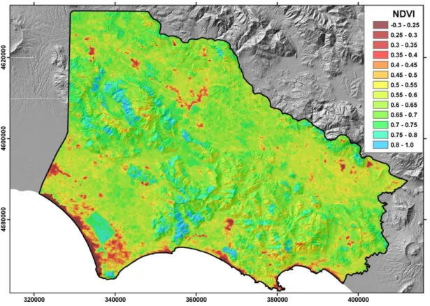
Although it shows a not very refined ground resolution (250 m), if compared to other satellite sensors, the MODIS platform has the advantage to guarantee a rather continuous coverage on long-term observations. Therefore, basing on the 15-days radiometric measurements, the mean annual NDVI layers were firstly generated in GIS environment for each year. Afterwards, a unique layer was created where each cell or pixel contains the mean NDVI averaged over the whole considered time-span (Fig. 2). To accomplish that, the raster calculator tool was utilized. In the figure, built areas and water bodies (coastal lagoons and lakes) are recognizable by reddish colors as well as the greenhouse area southward of the forest quadrangle of the National Park of Circeo.
14
Incidentally, it is interesting to examine whether significant changes have occurred in NDVI during the considered period. Figure 3 shows the diagram of the mean areal NDVI (yearly NDVI averaged on the whole study area) from 2001 to 2016. Fluctuations are limited within a narrow interval between 0.580 and 0.630 with a standard deviation close to zero , proving that no meaningful changes have occurred in NDVI, on average. Nonetheless, the diagram shows a clear growing trend of mean areal NDVI, within the aforementioned limits, which can be paired with the greening trend of natural vegetation, due to the increase of biomass and carbon in vegetation over a large part of the Italian territory. This trend was acknowledged in recent studies (Mancino et al 2014, Castellari et al 2014) and also confirmed by the last national forestry and agriculture inventories (INFC 2015; ISTAT 2013).
Fig. 3 - Diagram of mean NDVI and annual trend (dashed line).
Trying to understand the possible causes of this trend is not the main scope of the present work, nevertheless, it can be of interest to verify the range of possible climate changes occurred in the same period. Given the relationship of NDVI with vegetation cover, in fact, it follows that an indirect relationship can exist between NDVI and climate whose variations can affect vegetation conditions. To this aim, rain and temperature data from 2001 to 2016 year have been collected from gauging stations located at elevations ranging from 2 to 850 m a.s.l. and distances from the coast from 1 to 63 km (Fig. 4) 0.550 0.560 0.570 0.580 0.590 0.600 0.610 0.620 0.630 0.640 2001 2002 2003 2004 2005 2006 2007 2008 2009 2010 2011 2012 2013 2014 2015 2016 N D VI Years
15
Fig. 4 - Location of rain gauges and thermometric stations
In Figure 5, a comparative diagram of average rainfalls and temperatures versus NDVI is shown. As can be seen, on an average annual basis, no significant correlation holds between NDVI and temperature whilst a slightly more significant match with the rainfall trend can be recognized (Pearson's r = 0.444, p = 0.085 significant at 0.01 level). The slight growing trend of NDVI could be conceptually coupled with the increasing trend of rainfall, but it cannot be claimed on a statistical basis.
Another relationship can be investigated with land cover changes. The presence in the area of numerous scattered artifacts, i.e., farm houses, barns, warehouses, greenhouses and secondary roads can perturb the ground spectral response in adjacent natural vegetation and cultivation areas. By analyzing the frequency distribution of NDVI data in relation to the spatial distribution of artifacts in the area, it resulted that the NDVI values of 0.5 and 0.6 mark the limits between three main groups of land cover: total artificial and bare areas, with NDVI lower than 0.5; natural or
cultivation areas with no or little artifacts, with NDVI higher than 0.6; mixed areas (natural or
cultivation areas with significant presence of artifacts), with NDVI comprised between 0.5 and 0.6 (Fig. 6). In this latter interval, as previously shown in Fig. 3, small fluctuations of mean NDVI, averaged on the whole area, have occurred until 2012. After 2012, the mean NDVI increases over 0.61 which could be explained by a relative increase of natural areas surface, in agreement with the greening trend cited before.
16
Fig. 5 - Trend of mean annual NDVI, rainfall and air temperature in the period 2001-2016 (data series normalized by mean and standard deviation).
Fig. 6 - NDVI classification of the study area based on artifacts presence (red: total artificial
and bare/water areas; blue: natural or cultivation areas with no or little artifacts; olive-green: mixed areas). -2 -1.5 -1 -0.5 0 0.5 1 1.5 2 2001 2002 2003 2004 2005 2006 2007 2008 2009 2010 2011 2012 2013 2014 2015 2016 T P NDVI
17
5. Model analysis and application
The rationale of the present analysis is based on the consideration that the NDVI reflects the land cover variations in a one-to-one correspondence. This means that, as C-factor changes in space (from one cover-type to another or through the same cover-type) and time (from a minimum to a maximum during the year and from year to year), due to natural vegetation or crop and management variations, so does the NDVI, consequently.
Given the lack of C-factor data from long-term field observations in the area here considered, our approach in searching for a correlation model between NDVI and C-factor is based on correlating the mean NDVI from long-term satellite imagery with mean long-term C-factor data provided in the literature for different land cover types with reference to the same time-interval. This approach is justified by the proven low variability of mean area-NDVI in the considered period as shown in the previous section of present work. With these preliminary remarks, correlating average NDVI and C-factor data will allow to find a general law describing the statistical relationship between the two variables that will help to derive the C-factor from NDVI at different time-scales (yearly, seasonal and monthly).
The C-factor data here considered as baseline are those reported for Italy in the C-factor map of the European Union by Panagos et al. (2015c), representing average estimates derived from literature review, high spatial resolution remote sensing and statistical data on agricultural and management practices gathered in different pan-European databases such as Corine Land Cover, NUTS and MERIS.
In the present work, the effort was addressed to find the accurate correspondence between the data from the EU C-factor map and the NDVI data from MODIS by overlaying the two raster layers in GIS environment (the ArcGIS10® release has been used to this aim). To achieve that, given the different resolutions by the two layers (100 m the one and 250 m the other) it was necessary to make a downscaling in order to match them. Unfortunately, the different systems (RS) the two layers were are referred to (ETRS89 for the EU C-factor map and WGS84 for the NDVI) did not allow to obtain a perfect pixel overlay, after the RS transformation and homogenization, due to the persistence of errors and planar deformations. Therefore, it was preferred to compare the two raster layers on the basis of extended areas belonging to selected land cover classes, rather than cell by cell of the grid, in order to minimize the errors due to map offsets. By analyzing the C-factor frequency histogram, ten groups of values were identified by which the EU C-factor map was reclassified in homogeneous areas each of them was labeled with the corresponding C-factor average value. The area contours for each class were then overlaid on the NDVI map in order to capture the vegetation index data ranging within each class and calculate the corresponding mean value. Then, by the "extract by mask" tool available in the Spatial Analyst of the ArcTool box, the two series of objects were matched to obtain a unique attribute table containing the C-factor and NDVI mean values pairs. The data pairs were then put on a diagram, with NDVI on the x-axis versus the C-factor on the y-axis, in order to find the best interpolation model function.
Hypothesizing a linear relationship, as envisaged by De Jong (1994, 1998), the C-factor would decrease proportionally with increasing NDVI. However, as shown in Fig. 7, a linear model will tend to underestimate the C-factor in the central part of NDVI data distribution and to overestimate it when NDVI tends to the extremes of the same distribution, suggesting that a non-linear model would better approximate the observed data. Moreover, according to the non-linear model, NDVI values very close to 1 (0.8-0.9) would produce C-factor values less than zero, that is
18
physically inconsistent, according to the definition of the C-factor itself (Wischmeier & Smith 1978). Actually, when the NDVI gets closer to its maximum value 1 the C-factor is very close to zero but never null. This can be observed in an area under homogeneous forest cover such as the forest included in the National Park of Circeo, at the south-western edge of the study-area, where the C-factor is ranging from 0.0006 to 0.002 (Panagos et al., 2015c).
Fig. 7 - Linear model showing deviations from observed data.
Therefore, a correction factor must be introduced by which the regression model would be not represented by a straight line but by a curve better approximating the actual data trend. Moreover, a conditional constraint must also be introduced, fixing C = 0 for NDVI = 1, to avoid negative values. Furthermore, in the present case, the curve may be truncated at NDVI = 0.4 since, in the investigated area, lower values correspond to artificial and bare/water areas (Fig. 6) for which estimating the C-factor would not make sense. All things considered, a logistic sigmoid curve will represent the best interpolation line. The resulting model function has the form:
(8)
In the present case-study, the equation parameters show the values: a = 0.3439; b = 0.6137; c = - 0.0295. 0 0.05 0.1 0.15 0.2 0.25 0.3 0.35 0.4 0.45 0.45 0.5 0.55 0.6 0.65 0.7
C
NDVI
C = a + b*NDVI
19
Fig. 8 - Modeled function of C-factor vs. NDVI (dashed lines: 95% confidence interval).
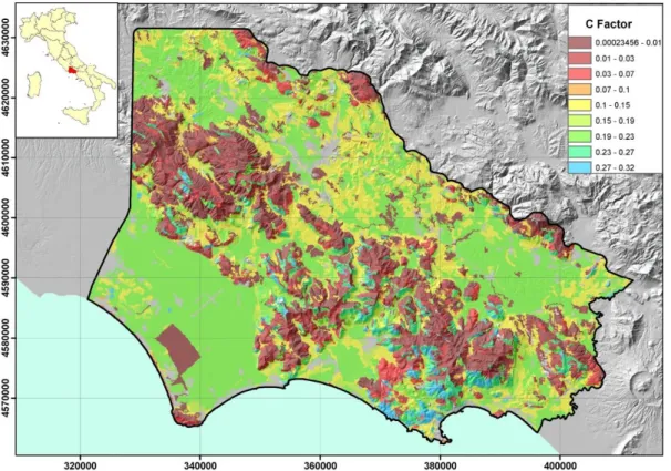
Fig. 9 - C-factor map of the area derived by equation (8). Urban areas and water bodies (in grey color) are excluded.
Figure 8 shows the fitted curve where none of the observed points lies outside the confidence interval. The model function so obtained was applied to the study-area, basing on the mean 2001-2016 year NDVI layer, in order to show the distribution of estimated mean long-term management factor in
0 0.05 0.1 0.15 0.2 0.25 0.3 0.35 0.4 0.4 0.5 0.6 0.7 0.8 0.9 1 C NDVI R2 = 0.989 Std. err. = 0.015 Sigmoid function Observed 95% confidence bounds
20
the area, with 250 m - spatial resolution (Fig. 9). In the figure, the estimated C-factor is classified following the same class-intervals as in the base-map by Panagos et al. (2015c) (Fig. 10) in order to compare the results.
Fig. 10 - C-factor map extracted from the EU map by Panagos et al. (2015c). Urban areas and water bodies (in grey color) are excluded.
By a quick look, compared to the EU-map, a major diffusion of medium-high classes seems to be evident in the map derived by applying equation (8). This differentiation appears more noticeable in large plain areas (Agro Pontino, Fondi plain and Valle Latina), meaning that, as far as croplands are concerned, the proposed model would overestimate the C-factor with respect to the EU-map. Elsewhere in the area, e.g., on the central mountain ridge and other areas of Valle Latina, slight underestimates can be observed. In Table 2, a direct comparison on statistical basis is shown. The correlation appears good for C-factor values lower than 0.1482, corresponding to forest and semi-natural areas (NDVI higher than 0.622). It worsens for values from 0.1482 to 0.2954 (agricultural areas) and get slightly better for greater values up to 0.369 (vineyards, olive groves and natural grasslands). These latter, however, show a very lesser areal extent than other land-use categories.
Analyzing the two maps in detail, if we consider the boundaries of the CLC2012 classes, one can see that the areas classified as arable lands show a data ranging very similar in the EU map and the map modeled by the eq. (8) (from 0.001 to 0.358 with standard deviation of 0.036 in the first, and from 0.001 to 0.344 and standard deviation of 0.097 in the second). Consequently, the corresponding average values for arable lands are very close (Table 3).
21
Table 2 - Correlation degrees between model results and EU-map for different C-factor class groups.
Lower bound Upper bound Spearman's coefficient 1 [0.001, 0.0746[ 0.53
2 [0.0746, 0.1482[ 0.62 3 [0.1482, 0.2218[ -0.04 4 [0.2218, 0.2954[ 0.04 5 [0.2954, 0.369] 0.27
Table 3 - Comparison between EU-map and model results averaged for CLC12 land cover classes
CLC2012
3rd level Description EU map Model eq. (8) 211 Non-irrigated arable land 0.212 0.183 222-223 orchards and berry plantations; Olive
groves
0.182 0.113
242 Complex cultivation patterns 0.140 0.171 243 Land principally occupied by agriculture,
with significant areas of natural vegetation
0.118 0.092
31x Broad-leaf forest; Coniferous forest; Mixed forest;
0.013 0.045
321 Natural grassland 0.174 0.191 322-23-24 Moors and heathland; Sclerophyllous
vegetation; Transitional woodland-shrub
0.133 0.097
Actually, the C-factor assigned to arable lands in the EU map has a uniform value of 0.221 for 94% of the cells composing that land-cover class, while the eq. (8) model values show a wide range around the average (Fig. 11), probably more realistically mirroring the varying cover degrees of different kinds of cultivations. To this aim, it must be pointed out that the C-factor for arable lands reported in the EU map is the result of C-factor estimates from literature review, averaging different crop types, combined with the effects of management practices.
With regard to forested areas (CLC2012 class 31x), the EU map shows a data ranging from 0.001 to 0.310 with standard deviation of 0.04 and average value of 0.013. The model eq. (8) gives for the same areas values from 0 to 0.344 with standard deviation of 0.067 and average value of 0.045. Also in this case, the difference between observed and estimated data is not substantial.
Ultimately, the diagram shown in Fig. 12, correlating the average C-factors reported in Table 3, allows to conclude that the EU-map and the map derived from eq. (8) show a good agreement (R2 = 0.64).
22
Fig. 11 - Frequency diagram of C-factor values for arable lands from model equation (8)
The uncertainties between the two maps may be explained considering the different techniques used, in the two model approaches, for deriving and representing the data. As an example, besides the different resolution, already recalled, the influence of artifacts on the NDVI spectral response in the "mixed areas", as pointed out above, can entail some deviations from the EU map reference values.
Fig. 12 - Correlation diagram between EU map average data and data from eq. (8) for CLC12 classes
All things considered, the estimates obtained by means of eq. (8) do not strongly conflict on average with the EU map. The most significant difference is that while the EU map provides a static value for C-factor, depicting the long-term effect of land cover (as it was detected in that considered time-interval), on the contrary, the proposed model will be able to catch the changes of the same variable with time.
R² = 0.64 0 0.05 0.1 0.15 0.2 0.25 0 0.05 0.1 0.15 0.2 0.25 C - m o d e le d b y e q . (8) C - EU map
23
24
25
For example, considering a couple of critical years, for the area here examined, such as 2007 and 2013 year, characterized, respectively, by the lowest and the highest yearly total rainfall in the whole 2001-2016 time span, the corresponding values assumed by the annual C-factor can be estimated (Fig.13). Consequently, the soil loss degree may also be assessed in those specific conditions. As can be seen, the C-factor in 2007 appears much higher than in 2016, on average, indicating a major proneness to soil erosion as consequence of minor vegetation growth under lower moisture conditions.
In the same way, a suitable C-factor can be assessed on a seasonal basis too. As an example, considering Autumn as the most critical season for croplands in the Mediterranean area, since soils are coverless and most vulnerable, in this part of the year, while rainfalls are heaviest, the C-factor maps are here reported for Autumn 2005 and 2006, when the maximum and the minimum rainfall have been recorded for that season in the studied area (Fig. 14). Actually, the resulting C-factor in the first case is lower than in the second, on average, as consequence of major vegetation development and soil coverage under higher moisture conditions.
6. Conclusions
An improved non-linear correlation model was developed to estimate the soil cover management factor of USLE/RUSLE basing on NDVI satellite observation data. Notwithstanding some uncertainties in the estimate, the model provided good results. The main benefit deriving from the model here developed will consist in the possibility to estimate the C-factor for large areas at differently refined time scales (from 15-days to yearly) and draw updated maps when needed, basing on the availability of NDVI data-series.
The choice of utilizing moderate-resolution satellite images, such as those provided by the MODIS platform, can be the origin of uncertainties between observed and derived C-factor values. However, the advantage in using such data is in their optimum coverage and temporal resolution with free availability. Most likely, satellite platforms with higher resolution could allow better results. This issue will be a topic for further research. On the other hand, high-resolution imageries could be economically onerous, which is a key-factor for many public administrations requiring to utilize satellite data as planning and management tool.
Acknowledgements
The present study was made possible thanks to the free availability of MODIS imageries, courtesy of the NASA Land Processes Distributed Active Archive Center (LP DAAC), USGS/Earth Resources Observation and Science (EROS) Center, Sioux Falls, South Dakota, https://lpdaac.usgs.gov/data_access/data_pool.
Thanks also to the ESDAC-European Soil Data Centre (esdac.jrc.ec.europa.eu), European Commission, Joint Research Centre, for making available the Cover Management factor (C-factor) map for the EU in digital format.
26
References
Angeli L, Costantini R, Ferrari R, Innocenti L, Costanza L (2007) Stima della sensibilità all'erosione del suolo attraverso l'analisi di scenari climatici. Atti 11^ conferenza nazionale ASITA, 6-9 novembre 2007 Torino (Italy)
Angulo-Martínez M, López-Vicente M, Vicente-Serrano SM, and Beguería S (2009) Mapping rainfall erosivity at a regional scale: a comparison of interpolation methods in the Ebro Basin (NE Spain). Hydrol. Earth Syst. Sci., 13: 1907-1920
ARPAV (2008) Valutazione del rischio d'erosione per la Regione Veneto. Gennaio 2008: 49 pp Bagarello V, Di Piazza GV, Di Stefano C, Ferro V (2008) Il fattore di erodibilità del suolo e la carta dell'erosione potenziale. In: Ferro (ed ) Linee guida per l'applicazione della USLE in ambiente Mediterraneo. Quaderni di Idronomia Montana 28/1, Nuova Editoriale Bios, Castrolibero (Cs): 55-70
Bayramov E, Jabbarli K (2013) GIS and Remote Sensing based environmental management of the Shirvan National Park in Azerbaijan. 2013 ESRI Europe, Middle East, and Africa Conference Proceedings, October 21–25, 2013 - Munich (Germany)
Binetti A (2011) Difesa del suolo attraverso l’uso del suolo: suggestioni per una rivisitazione del vincolo idrogeologico ex RD 3267/23. Atti 15a Conferenza Nazionale ASITA - Reggia di Colorno 15-18 novembre 2011: 349-360
Borselli L (1993) Temporal changes in soil erodibility. Quaderni di Scienza del Suolo, vol. V: 23-46
Borselli L, Torri D, Poesen J, Iaquinta P (2012) A robust algorithm for estimating soil erodibility in different climates. Catena, 97: 85–94
Braunović S, Bilibajkic S and Ratknic M (2010) Calculation of rainfall erosivity factor in the Region of Vranje (South-Eastern Serbia). In: Zlatic M (ed.) Global change - challenges for soil management. Catena-Verlag: 184-191
Buttafuoco G, Conforti M, Aucelli P Robustelli G, Scarciglia F (2011) Assessing spatial uncertainty in mapping soil erodibility factor using geostatistical stochastic simulation. Environ Earth Sci DOI 10.1007/s12665-011-1317-0
Cartagena DF (2004) Remotely Sensed Land Cover Parameter Extraction for Watershed Erosion Modeling. M.Sc. Thesis, International Institute for Geo-Information and Earth Observation, Enschede (The Netherlands), 104 pp
Castellari S., Venturini S., Ballarin Denti A., Bigano A., Bindi M., Bosello F., Carrera L., Chiriacò M.V., Danovaro R., Desiato F., Filpa A., Gatto M., Gaudioso D., Giovanardi O., Giupponi C., Gualdi S., Guzzetti F., Lapi M., Luise A., Marino G., Mysiak J., Montanari A., Ricchiuti A., Rudari R., Sabbioni C., Sciortino M., Sinisi L., Valentini R., Viaroli P., Vurro M., Zavatarelli M. (a cura di.) (2014). Rapporto sullo stato delle conoscenze scientifiche su impatti, vulnerabilità ed adattamento ai cambiamenti climatici in Italia. Ministero dell’Ambiente e della Tutela del Territorio e del Mare, Roma, Italy, 878 pp
27
De Jong SM (1994) Derivation of vegetative variables from a Landsat TM image for modelling soil erosion. Earth Surface Processes and Landforms, vol. 19: 165-178
De Jong SM, Brouwer LC, Riezebos HTh (1998) Erosion hazard assessment in the Peyne catchment, France, Working paper DeMon-2 Project, Dept. Physical Geography, Utrecht University.
Desmet P and Grovers G (1996) A GIS procedure for automatically calculating the USLE LS factor on topographically complex landscape units. Journal of Soil and Water Conservation, 51(5): 427 – 433
Durigon VL, Carvalho DF, Antunes MAH, Oliveira PTS & Fernandes MM (2014) NDVI time series for monitoring RUSLE cover management factor in a tropical watershed. International Journal of Remote Sensing, 35/2: 441-453
Erencin Z (2000) C-Factor Mapping Using Remote Sensing and GIS. Thesis, Geographisches Institut der Justus-Liebig Universität Giessen (Germany) and International Institute for Aerospace Survey and Earth Sciences, Enschede (The Netherlands), 28 pp
Giovannozzi M, Martalò PF, Mensio F (2013) Carta dell’erosione reale del suolo a scala 1:250 000 Regione Piemonte.
http://www.regione.piemonte.it/agri/psr2007_13/dwd/servizi/note_carta_erosione_reale_suoli.pdf. Grimm M, Jones RJA , Rusco E and Montanarella L (2003) Soil Erosion Risk in Italy: a revised USLE approach. European Soil Bureau Research Report No 11, EUR 20677 EN, (2002)
Guermandi M, Staffilani F (2006) Carta del rischio di erosione idrica e gravitativa - Relazione metodologica. http://ambiente.regione.emilia-romagna.it/geologia/archivio_pdf/webgis-banche dati/erosionesuolo/poster_Carta_Erosione_PSR.pdf
Hickey R, Smith A and Jankowski P (1994) Slope length calculations from a DEM within Arc/Info GRID. Computers, Environment, and Urban Systems, 18(5): 365 - 380
Hickey R (2000) Slope Angle and Slope Length Solutions for GIS. Cartography, v. 29, no. 1: 1 - 8
Higginbottom T and Symeonakis E (2014) Assessing Land Degradation and Desertification Using Vegetation Index Data: Current Frameworks and Future Directions. Remote Sensing, 6: 9552-9575. doi:10.3390/rs6109552
INFC Italian national forest inventory (2015) http://www.sian.it/inventarioforestale/
ISTAT Italian National Institute of statistics (2013) 6° General Census of Agriculture http://censimentoagricoltura.istat.it/
Jamshidi R, Dragovich D, Webb AA (2014) Catchment scale geostatistical simulation and
uncertainty of soil erosdibility using sequential Gaussian simulation. Environ. Earth Sci., 71: 4965-4976
Karaburun A (2010) Estimation of C factor for soil erosion modeling using NDVI in Buyukcekmece watershed. Ozean Journal of Applied Sciences 3(1): 77-85
28
Kouli M, Soupios P, Vallianatos F (2009) Soil erosion prediction using the Revised Universal Soil Loss Equation (RUSLE) in a GIS framework, Chania, Northwestern Crete, Greece. Environ Geol (2009) 57: 483–497. DOI 10.1007/s00254-008-1318-9
Lark RM, Cullis BR, Welham S J (2006) On spatial prediction of soil properties in the presence of a spatial trend: the empirical best linear unbiased predictor (E-BLUP) with REML. European Journal of Soil Science, 57: 787-799
Mancino G, Nolè A, Ripullone F, Ferrara A (2014) Landsat TM imagery and NDVI differencing to detect vegetation change: assessing natural forest expansion in Basilicata, southern Italy. iForest 7: 75-84
Mitasova H, Hofierka J, Zlocha M and Iverson L (1996) Modelling topographic potential for erosion and deposition using GIS. International Journal of GIS, 10(5): 629 - 641
Moore ID and Wilson JP (1992) Length-slope factors for the revised universal soil loss equation: simplified method of estimation. Journal of Soil and Water Conservation, 47(5): 423-428
Panagos P, Karydas CG, Gitas IZ, Montanarella L (2012) Monthly soil erosion monitoring based on remotely sensed biophysical parameters: a case study in Strymonas river basin towards a functional pan-European service. International Journal of Digital Earth Vol. 5, Iss. 6, 2012, pp. 461-487
Panagos P, Karydas CG, Ballabio C, Gitas IZ (2014a) Seasonal monitoring of soil erosion at regional scale: An application of the G2 model in Crete focusing on agricultural land uses.
International Journal of Applied Earth Observations and Geoinformation 27PB (2014), pp. 147-155, DOI: 10.1016/j.jag.2013.09.012.
Panagos P, Karydas CG, Borrelli P, Ballabio C, Meusburger K (2014b) Advances in soil erosion modelling through remote sensing data availability at European scale. Second International Conference on Remote Sensing and Geoinformation of the Environment (RSCy2014), Proc. of SPIE Vol. 9229 92290I, DOI: 10.1117/12.2066383
Panagos P, Borrelli P, Poesen J, Ballabio C, Lugato E, Meusburger K, Montanarella L, Alewell C (2015a) The new assessment of soil loss by water erosion in Europe. Environmental Science & Policy, 54: 438–447
Panagos P, Borrelli P, Meusburger K, van der Zanden EH, Poesen J, Alewell C (2015b) Modelling the effect of support practices (P-factor) on the reduction of soil erosion by water at European scale. Environmental Science & Policy, 51: 23-34 http://dx.doi.org/10.1016/j.envsci.2015.03.012
Panagos P, Borrelli P, Meusburger K, Alewell C, Lugato E, Montanarella L (2015c) Estimating the soil erosion cover-management factor at the European scale. Land Use Policy journal 48C : 38-50 doi:10.1016/j.landusepol.2015.05.021
Parveen R and Kumar U (2012) Integrated Approach of Universal Soil Loss Equation (USLE) and Geographical Information System (GIS) for Soil Loss Risk Assessment in Upper South Koel Basin, Jharkhand. Journal of Geographic Information System, 2012, 4: 588-596
29
Patil RJ and Sharma SK (2013) Remote Sensing and GIS based modeling of crop/cover management factor (C) of USLE in Shakker river watershed. International Conference on Chemical, Agricultural and Medical Sciences (CAMS-2013) Dec. 29-30, 2013 Kuala Lumpur (Malaysia): 1-4 Perović V, Životić L, Kadović R, Ðorđević A, Jaramaz D, Mrvić V, Todorović M (2012) Spatial modelling of soil erosion potential in a mountainous watershed of South-eastern Serbia. Environ Earth Sci. DOI 10.1007/s12665-012-1720-1
Piccini C, Marchetti A, Santucci S, Chiuchiarelli I, Francaviglia R (2012) Stima dell’erosione dei suoli nel territorio della regione Abruzzo. Geologia dell’Ambiente, Supplemento al n° 2/2012: 257-261
Prasannakumar V, Shiny R, Geetha N, Vijith H (2011) Spatial prediction of soil erosion risk by remote sensing, GIS and RUSLE approach: a case study of Siruvani river watershed in Attapady valley, Kerala, India. Environ Earth Sci, 64: 965-972
Renard KG, Foster GR, Weesies GA, Porter PJ (1991) RUSLE-revised universal soil loss equation. Journal of Soil and Water Conservation 46: 30-33
Renard KG , Foster GR , Weesies GA , McCool DK , Yoder DC (1996) Predicting soil erosion by water - a guide to conservation planning with the revised universal soil loss equation (RUSLE). United States Department of Agriculture, Agricultural Research Service (USDA-ARS) Handbook n° 703, Washington, DC
Römkens MJM, Prasad S.N. and Poesen JWA (1986) Soil erodibility and properties. Proc. 13th Congr. Int. Soil Sci. Soc., Vol. 5: 492-504
Rusco E, Montanarella L, Tiberi M, Rossini L, Ricci P, Ciabocco G, Budini A, Bernacconi C (2007) Implementazione a livello regionale della proposta di direttiva quadro sui suoli in Europa. European Commission - Joint Research Centre, EUR 22953 IT, ISSN 1018-5593: 65 pp
Salvador Sanchis M P, Torri D, Borselli L and Poesen J (2008) Climate effects on soil erodibility. Earth Surf. Process. Landforms 33: 1082-1097
Terranova O, Antronico L, Coscarelli R, Iaquinta P (2009) Soil erosion risk scenarios in the Mediterranean environment using RUSLE and GIS: An application model for Calabria (southern Italy). Geomorphology, 112, doi:10 1016/j geomorph 2009 06 009: 228-245
Torri D, Poesen J, Borselli L (1997) Predictability and uncertainty of the soil erodibility factor using a global dataset. Catena, 31: 1-22
Van der Knijff JM, Jones RJA & Montanarella L (1999) Soil erosion risk assessment in Italy. European Soil Bureau - JRC, EUR 19022 EN 54 pp
Van der Knijff JM, Jones RJA & Montanarella L (2000) Soil erosion risk assessment in Europe. European Soil Bureau - JRC, EUR 19044 EN 34 pp
Van der Knijff JM, Jones RJA & Montanarella L (2002) Soil erosion risk assessment in Italy. Proceed. 3rd Int. Congress ISSS Valencia (J.L. Rubio, R.P.C. Morgan, S. Asins & V. Andreu, eds.), Geoforma Ediciones: 1903-1917
30
Van Leeuwen WJD and Sammons G (2003) Seasonal land degradation risk assessment for Arizona. In: Proceedings of the 30th International Symposium on Remote Sensing of Environment, ISPRS: 378-381
Van Remortel R, Hamilton M and Hickey R (2001) Estimating the LS factor for RUSLE through iterative slope length processing of digital elevation data. Cartography, 30, n°1: 27-35
Van Remortel RD, Maichle RW, Hickey RJ (2004) Computing the LS factor for the Revised Universal Soil Loss Equation through array-based slope processing of digital elevation data using a C++ executable. Computers & Geosciences 30: 1043-1053
Van Camp L, Bujarrabal B, Gentile AR, Jones RJA, Montanarella L, Olazabal C and Selvaradjou SK (2004) Reports of the Technical Working Groups Established under the Thematic Strategy for Soil Protection. EUR 21319 EN/2, Office for Official Publications of the European Communities, Luxembourg, 872 pp
Wang G, Gertner G, Liu X, Anderson A (2001) Uncertainty assessment of soil erodibility factor for revised universal soil loss equation. Catena, vol. 46, issue 1: 1–14
Wischmeier WH, Smith DD (1978) Predicting rainfall erosion losses: a guide to conservation planning. United States Department of Agriculture Handbook n°537, United States Government Printing Office, Washington, DC
Young RA, Römkens MJM, McCool DK (1990) Temporal variations in soil erodibility. Catena supplement, 17: 41-53
ENEA
Servizio Promozione e Comunicazione
www.enea.it
Stampa: Laboratorio Tecnografico ENEA - C.R. Frascati giugno 2018