Benefits to Vulnerable Consumers in Italian Energy Markets: A Focus on the Eligibility Criterion

See discussions, stats, and author profiles for this publication at: https://www.researchgate.net/publication/274194410

Benefits to vulnerable consumers in Italian energy markets: a focus on the eligibility criterion Chapter · May 2016 CITATION 1 READS 202 3 authors:

Some of the authors of this publication are also working on these related projects:

Multi-unit Auctions’ Design in Electricity Markets: new challenges after the growth of renewable power plant capacityView project

Public Utilitiies: Affordability measures and vulnerable consumers' supportView project Raffaele Miniaci

Università degli Studi di Brescia

74PUBLICATIONS   878CITATIONS   

SEE PROFILE

Carlo Scarpa

Università degli Studi di Brescia

91PUBLICATIONS   880CITATIONS   

SEE PROFILE

Paola Valbonesi

National Research University Higher School of Economics (HSE)

120PUBLICATIONS   649CITATIONS   

SEE PROFILE

All content following this page was uploaded by Paola Valbonesi on 02 April 2015. The user has requested enhancement of the downloaded file.

1

Benefits to vulnerable consumers in Italian energy markets:

a focus on the eligibility criterion

Raffaele Miniaci – Carlo Scarpa – Paola Valbonesi

ABSTRACT: We discuss alternative approaches to define and measure the affordability of energy consumption. We then focus on energy vulnerability in Italy and on the benefit schemes that compensate households in needs for their spending on energy services. We identify the potential beneficiaries of these subsidies in 2012 and investigate if their eligibility criterion is effective in

targeting public resources to families in a state of energy vulnerability. (67 words)

Keywords: fuel poverty; affordability; utility tariffs; vulnerable consumers, eligibility criterion JEL: D12, I32, I38, Q4

1. Introduction

In this study, we aim at providing evidence on vulnerable consumers in the Italian domestic energy markets. By exploiting a large household survey and alternative indices, we investigate electricity and gas affordability in 2012; we then illustrate the Italian program of gas and electricity benefits in support of low-income households and assess its ability to actually target the households in needs.

In this perspective, we shortly present the debate about the concepts of affordability and the statistical indices that are typically adopted to assess the issue. Each approach can produce a somehow different picture of households’ vulnerability in energy consumptions and the recent report by Hills (2012) provides evidence of the lively debate on this issue. The key point is that the ideal affordability indicator should accommodate - with appropriate weights – numerous elements. On the one hand, it should be sensitive to changes in supply side variables (i.e. energy prices, technology, quality of service) and, on the other one, it must take into consideration consumers’ needs and preferences. This seems to be a particularly complex goal, given the heterogeneity of the households’ living conditions (e.g. climate, type of housing), and composition (e.g. number of family members, presence of children and/or elderly and disabled).

forthcoming in Jon Strand (ed.): The Economics and Political Economy of Energy Subsides, The MIT Press.

2

Based on our discussion on the pros and cons of the different affordability measures, we look at the affordability issue in the Italian domestic energy markets in 2012, using the annual European Union Surveys on Income and Living Conditions (SILC). On this database, we implement indices of affordability based on the incidence of the energy expenditure on the Italian family budget, as well as two ad hoc variations of the Low Income High Cost (LIHC) index proposed by Hills for fuel poverty in the UK. Moreover, we also consider self-assessed indicators of energy vulnerability, such as the presence of leaking roofs or broken windows, the inability to keep the house adequately warm and the presence of arrears for utility bills. As expected, the picture one gets on the extent of energy affordability problems substantially depends on how one defines and measures it.

Finally, we evaluate the effectiveness of the energy benefit system introduced in Italy in 2008. In particular, we investigate to what extent the eligibility rules really benefit households with energy affordability problems. Our results highlight that the eligibility rules are affected by several limitations: overall, about 15% of the households in absolute poverty do not meet the criteria, only 43% of the households at risk of poverty and no more than 61% of those with energy affordability problems qualify for the benefits

The rest of paper is organized as follows. In Section 2, we present alternative measures of affordability. In Section 3, we describe the Italian program of energy benefits. In Section 4 we empirically investigate the measures of affordability on Italian data; we then consider the potential beneficiaries of the Italian energy benefits providing estimates of the probability of being eligible, given that the household is energy poor. Policy implications are then discussed in the Conclusions (Section 5).

2 Energy affordability indicators and their measurement

In this Section we first present the most common affordability measures, based on the incidence of energy spending on total household expenditure or income (subsection 2.1); we then illustrate indicators based on the LIHC approach suggested by Hills (2012), also proposing some modifications (subsection 2.2).

2.1 Affordability indices based on energy budget shares

The general idea behind this approach is that energy consumption is part of an essential basket of consumption goods, which every household should be able to afford in order to have a

3

“normal” standard of living, characterized by normal heating conditions and consumption of household appliances services. In practice, a household is considered to face an affordability issue if its energy budget share exceeds a critical threshold, determined – more or less arbitrarily – by the policy makers. Accordingly, that household should be considered as part of the target population of any policy aimed at reducing energy poverty.

In this context, a headcount index is the percentage of consumers who spend on energy more than a given fraction of their income or total expenditure. In most studies, this critical threshold

has been fixed between 5% and 10%, depending on the good/service considered.1 In so doing,

such index – as the underlying concept of affordability – does not incorporate any information about the desirable minimum amount of consumption of energy and other goods.

Formally, define xh the total observed expenditure for household h, corresponding to the sum

of the expenditure in energy, u

h

x , and the actual expenditure in all other consumption items, x_hc.

According to this approach, a household has problems of sustainability of its energy consumption

if the ratio h

u h

h x x

r  / is larger than a given threshold ru. Considering a population, the extent of

the sustainability problem is measured by the fraction of households for which u

h r

r  , i.e. by the

Headcount Index (HI):

[1]



u



h h r r HI N  



1

where N is the total number of households and



u



h

r r

1 is an indicator function, which equals

one whenever the condition in parentheses holds, and zero otherwise. The index HI in [1] tells us the fraction of the households which spend more than a given "reasonable amount" (in proportion to available resources) for energy consumptions. Notice that [1] does not incorporate any qualitative information on the amount of minimum/ desirable consumption, both for energy and for other goods or services.

However, such notion cannot provide useful indications on either the extent of the affordability problem, or its depth. As for the former issue, it does not include among the fuel poor those households in absolute poverty that decide – because of economic constraints - to spend very little on energy services. Moreover, it can label as “fuel poor” some relatively well-off households

1

See about Fankhauser and Tepic (2007), Chaplin and Freeman (1999), Hancock (1993), Healy (2001), Sefton, (2001), Sefton and Chesshire, (2005), Waddams Price et al. (2012).

4

that are characterized by high energy consumption. 2

2.2 Affordability indices based on Low Income High Cost (LIHC) approach

As highlighted in Miniaci et al. (2008a, 2014b), the indices based on the budget share completely neglect the fact that spending in energy services can become problematic when it leaves a household insufficient income to consume other goods or services, namely when the household’s “residual income” is too low. Considering a residual income approach, there is a problem of energy affordability if - after paying the energy bills - the household does not have

sufficient financial resources to fund the minimum level of consumption of other goods/services.3

Note that this approach highlights the financial difficulties induced by the consumption of public utilities (Stone, 1993). This approach permits to disentangle at least three types of households whose affordability problems have different origins:

(i) households unable to access the minimum amount of both essential commodities and energy services: in this case, the problem of energy affordability can be alleviated by a mechanism of general income support, not conditional to the actual level of energy consumption;

(ii) households with limited income, which over-consume energy: in this case, an appropriately targeted action should address the reason why this happens (i.e. preferences, technological constraints, inefficient equipment, etc.);

(iii) households whose energy consumption is below the minimum standard due to monetary or non-monetary constraints (e.g. , lack of access to gas or electricity networks): in this case, interventions should first be aimed at removing these constraints.

The Low Income High Cost (LIHC) approach suggested by Hills (2012) combines elements of the residual income approach discussed above, with those of the budget share approach introduced in

the previous subsection. In particular, the LIHC approach classifies households as energy poor if:

- their disposable income minus the necessary spending in energy results lower than the

European Union relative poverty line,4 and

- the ratio between their necessary spending in energy over their disposable income results

lower than the median national energy budget share,

2

The problem of affordability in energy consumption has been firstly investigated in UK where it has been labelled as “fuel poverty” (see Defra 2001 and 2007).

3

The field where the notion of residual income was first introduced is housing economics (Thalmann, 2003).

4

The EU relative poverty line may differ from the relative poverty lines computed by the national statistical offices because of the different equivalence scales adopted.

5

where the necessary spending in energy is the expenditure needed to keep the house adequately warm, irrespectively of actual energy consumption. By referring to necessary rather than to actual energy expenditure, this approach avoids to “misclassify” those households that over-consume energy without needing to, as well as those that under-consume energy but that would need to consume more to live in an adequately heated home. Although appealing, Hills’ approach can hardly be implemented to countries other than the UK, for at least two reasons:

- it is particularly data demanding, as it requires an accurate estimate of households' energy

needs given the characteristics of their accommodations, data that are often unavailable in continental Europe and in the US;

- it refers to national median energy budget shares, which may be appropriate when applied to

an area/country where climatic conditions are relatively homogeneous.

We thus consider a modified version of the LIHC approach, where we use actual energy expenditure (rather than necessary spending) and, given the territorial variety of the Italy, we use regional specific budget share thresholds.

Formally, consider an household h with an actual level of energy expenditure u

h

x ; this

household has a residual income 𝑅𝐼ℎ , defined as RIh xhxhu, that is the difference between its

total disposable income 𝑥ℎ and its energy expenditure xuh. Such an household is energy poor

according the LIHE approach if its residual income falls below the relative poverty line xrp and its

energy budget share r_h xu_h /x_h is larger than a given threshold r . The headcount index u

associated with the modified LIHC approach, say LIHC1, is:

[2] LIHC1

1



h hu rp

 

h u



h

HI

x

x

x

r

r

N





1







1



In our opinion, both the original LIHC and its revised version LIHC1 suffer of the same problem: in order to assess the households’ ability to pay, they both refer to relative poverty rather than to absolute poverty and the residual income (i.e., net of energy costs) is compared to full income (that includes resources for energy spending). By doing so, the criteria do not consider as deprived those households with low income and low (necessary or actual) energy expenditure. In other words, the criteria are likely to exclude from the set of vulnerable consumers those households, whose lack of income induces them to spend too little in energy services.

In order to avoid misclassifying these households in need, we suggest a further modification to the LIHC criterion, according to which we consider as vulnerable those household:

6

- whose their disposable income is lower than the absolute poverty line, or

- the ratio of their actual spending in energy over their disposable income results larger than the

regional specific median energy budget share.

The headcount index associated with this modified LIHC approach, say LIHC2, is:

[2] LIHC1

1



h ap

 

h u

 

h ap

 

h u



h

HI

x

x

r

r

x

x

r

r

N









_

1





1





1





1



_

where xap denotes the absolute poverty line.

By using the LIHC2 criterion, we would include all the households that cannot afford the minimum quantity of energy without consuming too little of the other goods (first criterion), plus the households that consume “too” high a fraction of their income for energy. So, while LIHC1 tends to excludes poor households not spending enough on energy, LIHC2 tends to include some high-income household spending too much on energy.

3 Electricity and gas benefits in Italy

The Italian policy concerning benefits for electricity and gas to vulnerable consumers has been set forth by the Law 205 of 23 December 2005, and then implemented through two Ministerial Decrees in 2007 for electricity and 2008 for gas. The declared aim of the policy is to provide support in energy consumption to:

i) households living in poverty - or on its margins;

ii) large households.

And in case of electricity, also to:

iii) households which include a disabled, or a critically ill person (i.e. using medical device).

The policy is funded through specific components in transmission or distribution, paid by all consumers.

The income eligibility criteria for electricity and for gas benefits are the same; in both cases, the spending ability of the family is tested by using a synthetic indicator called ISEE (the acronym for “Indicatore di Situazione Economica Equivalente”, that is, Equivalent Economic Conditions Indicator). This indicator combines information about income, real and financial assets, family

7

composition and occupational status of household members. To be eligible, the household's equivalent income indicator must not exceed 7,500 Euro, unless the family includes more than three dependent children; in this case the threshold is increased to 20,000 euro.

Given that the benefits are paid in the form of lump-sum discounts on the electricity and gas bills, a necessary eligibility condition is that the household must be a domestic customer in its primary residence. In case of electricity, some limits to the installed power must be met (3 kW for up to 4 household members, 4.5 kW if more), unless the household includes a person who needs essential electro-medical appliances. In the case of gas, the benefit is given to the eligible households in the form of discount in bills for domestic customers having an individual contract, and with a postal order for customers having a condominium contract (i.e. usually due to the presence of centralised heating).

All domestic customers that meet the above criteria can apply for the benefits by filing a form to the municipality of residence. Given that the eligibility criteria are independent of consumption levels, the ubiquity of the power grid guarantees that (de facto) all households meeting the above income requisites are potential beneficiaries of the electricity benefit. The coverage of the gas benefit is instead jeopardized by the non-universal diffusion of the natural gas. In particular, the gas distribution grid does not serve many mountainous areas and the entire Sardinia region. This in practice makes the pool of eligible households for the gas benefit a subset of the households eligible for the electricity benefit.

The amount of the electricity benefit depends on the number of households components and it is independent of actual consumption (with the exception of the presence of electro-medical appliances, where it is calculated on the ground of the electricity usage intensity). In 2012, it ranged between 63 euro per year for a couple and 139 euro for a household with more than 4 members (plus 10% VAT). The amount of gas benefit is proportional to family size and depends on the classification of the municipality according to its typical winter temperature, and to the adoption of natural gas for heating. In this case, the value of the benefit ranged from 85 euro for a household with less than 5 members living in the warmest part of the county, to 318 euro for a household with at least 5 members living in the coldest areas (plus 21% VAT). Notice that the design of the gas benefit implies that households heating their homes with fuels other than natural gas are implicitly penalized by this system.

8

4 Energy poverty and energy benefits in Italy

To describe the incidence of energy poverty in Italy using the alternative approaches introduced in Section 2, and to assess to what extent the benefits’ policy described in Section 3 is actually capable of channelling resources toward vulnerable consumers, we first need to define some parameters for the empirical analysis as follows.

4.1 Setting the parameters for the empirical analysis

In the aim to apply the above measures of energy affordability to Italy, we have to set two

preliminary steps:

(i) define the relative and absolute poverty lines (xrp and xap, respectively), (ii) define the threshold ( u

r ) above which the budget share indicates the presence of an affordability problem.

We exploit the Eurostat - Istat “Survey on Income and Living Conditions” (EU-SILC) to estimate these crucial values according to a variety of criteria. This survey is particularly suitable for this aim, as it provides information on demographic, housing, occupational, and income variables for a representative sample of about 20,000 Italian households.

Table 1 shows some preliminary descriptive statistics to frame the Italian context, i.e. the average

monthly disposable income5 and the expenditure for energy, by household size and climatic

classification of the area of residence in Italy, in 2012. As already noticed in Miniaci et al (2008a, 2008b, 2014), the expenditure for gas and other fuels shows a significant variability across climatic areas: a family of two components in a cold region spends more that the double that a similar family in a warm region. For electricity instead, it is the number of household members that mainly affects the level of expenditure, while the area of residence plays a limited role.

5

Disposable income is defined as the household income, net of taxes and contribution to the social security system, including imputed rents.

9

Table 1: Average monthly disposable income and expenditure for energy, by household

size and climatic classification of the area of residence.

Disposable income

# hh members Warm Mild Temperate Cold Total 1 1501.84 1893.44 1829.49 2026.90 1883.36 2 2219.11 2897.49 2816.17 3328.81 2984.20 3 2673.25 3363.66 3715.36 3980.92 3556.29 4 2966.35 3722.64 3911.38 4503.47 3863.51 5 + 3073.76 3907.92 4410.94 4459.07 3930.55 Total 2340.11 2895.95 2950.12 3238.69 2953.29 Electricity expenditure

# hh members Warm Mild Temperate Cold Total

1 36.38 31.30 29.08 30.32 31.37 2 50.29 42.07 39.65 41.74 42.87 3 59.73 52.44 47.04 50.19 52.09 4 61.64 53.09 54.46 58.35 57.34 5 + 67.38 59.50 64.59 61.69 63.20 Total 52.14 43.87 41.48 42.78 44.61

Gas and other fuels expenditure

# hh members Warm Mild Temperate Cold Total

1 34.71 56.74 60.50 91.06 70.17 2 47.92 71.21 82.81 119.40 92.33 3 53.01 78.55 87.56 118.44 92.80 4 57.52 75.99 90.07 125.22 92.20 5 + 59.15 78.94 105.90 126.45 93.70 Total 48.24 69.63 79.20 110.89 85.59 Source: Istat “Survey on Income and Living Conditions” (EU-SILC), 2012.

Table 2: Average monetary value of the minimum reference for total monthly expenditure and energy

components, by household size and climatic classification of the area of residence.

Relative Absolute poverty line

# hh members poverty line Warm Mild Temperate Cold Total

1 740.71 603.19 707.96 709.10 797.64 733.91 2 1234.51 854.86 973.28 978.03 1102.34 1017.01 3 1641.90 1108.65 1231.26 1240.16 1399.71 1284.43 4 2012.26 1358.23 1489.40 1472.06 1698.63 1535.10 5 + 2434.20 1605.91 1752.95 1798.02 2010.59 1808.53 Total 1353.79 1002.09 1081.77 1067.36 1180.91 1109.51 Source: Istat “Survey on Income and Living Conditions” (EU-SILC), 2012.

10

Table 2 presents the relative poverty line and the average monthly absolute poverty line, by household size and climatic classification of the area of residence. We compute the relative income poverty line mimicking the definition of the expenditure poverty line for Italy adopted by the Italian Statistical Office (Istat). That is, the poverty line for a two-member household is equal to the average per capital household disposable income, and the value for other family size is adjusted using the Carbonaro equivalence scale. The disposable income is calculated as household income net of taxes and contribution to the social security system, and including imputed rents. The absolute poverty line for each family sampled by the survey is set following the definition of official Italian poverty line (Istat 2009), and it is, by construction, regional specific.

Different options are available in order to define the values of the threshold ru necessary to

define the measure based on the budget shares approach. In the present analysis, we consider

two criteria:

a) A “median budget share” approach, that looks at the balance sheets of households with low purchasing power and defines the maximum sustainable threshold ( u

r ) as the median value of the share of energy expenditure for the households in relative poverty. This threshold is conditional on household size and geographical area and varies over time due to changes in relative prices and household consumption decisions.

b) An “European Commission (EC) criterion”, that leads to a measure mimicking what has been

used in a European Commission Report (2010), i.e. the threshold is twice the ratio between the average energy expenditure over the average total expenditure. We implement this criterion with two modifications: 1) using disposable income instead of total expenditure, and 2) using averages (of both expenditure and disposable income) conditional on household size and climatic area.6

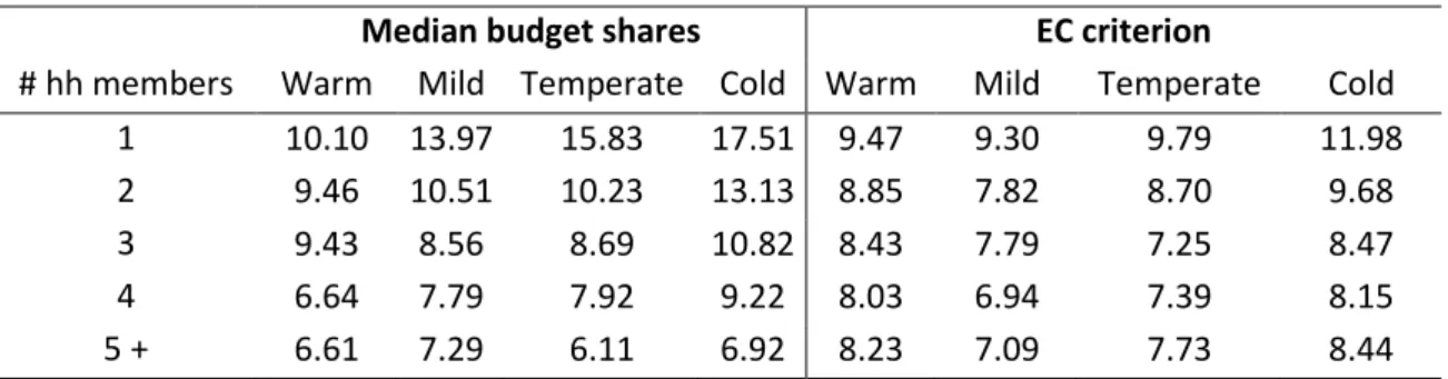
Table 3 shows the difference between thresholds computed according to criteria (a) and (b). In

particular, the table highlights that for households up to four members the threshold calculated according to the median budget shares approach are higher than those calculated with the EC criterion. As a consequence, we expect the incidence of energy poverty to appear to be lower when the threshold is set in accordance to the median budget share approach rather than the EC criterion.

6

The first modification is dictated by the lack of a reliable measure of total expenditure in the EU-SILC dataset, and in any case, income is probably a more sensible denominator in such ratio. The second modification is suggested by the large differences in Italian energy spending across areas and family size, as shown in Table 1.

11

Table 3: Critical thresholds ru for budget share approach. Median budget shares: median budget shares of the relatively poor, by household size and climatic classification of the area of residence. EC criterion: 2* Average expenditure / Average income, by household size and climatic classification of the area of residence.

Median budget shares EC criterion

# hh members Warm Mild Temperate Cold Warm Mild Temperate Cold 1 10.10 13.97 15.83 17.51 9.47 9.30 9.79 11.98

2 9.46 10.51 10.23 13.13 8.85 7.82 8.70 9.68

3 9.43 8.56 8.69 10.82 8.43 7.79 7.25 8.47

4 6.64 7.79 7.92 9.22 8.03 6.94 7.39 8.15

5 + 6.61 7.29 6.11 6.92 8.23 7.09 7.73 8.44

Source: Istat “Survey on Income and Living Conditions” (EU-SILC), 2012.

4.2 Setting the affordability of energy consumption and the benefits’ coverage

As already mentioned, we exploit the EU-SILC data to empirically investigate the incidence of energy poverty in Italy as captured by alternative approaches presented in Section 2. Moreover, to assess to what extent the benefits’ policy - described in Section 3 - is actually capable of channelling resources toward vulnerable consumers, we also make use of the Istat estimate of taxable labour income for each household in the survey; this information is necessary to compute the Equivalent Economic Conditions Indicator (ISEE), and therefore the eligibility status for the energy benefits.

Unfortunately, the EU-SILC dataset has some limitations. First, information on real and financial assets is not as detailed as information on income sources. Therefore the amount of real and financial wealth can only be estimated on the basis of fiscal and financial income data (see Miniaci et al. 2014, see Appendix C, for details). Second, the data do not reliably identify the households that could benefit of the electricity benefit for health reasons; therefore, we will focus exclusively on the eligible households of electricity benefits for economic hardship, which anyway are the vast majority of the entire audience. Third, some approximation is necessary also for gas; in fact, the questionnaire does not distinguish between the use of natural gas and other kinds of gas (e.g., LPG), thereby leading to an overestimation of the pool of eligible customers.

Table 4 presents average income, percentage of income poor, eligible households, and households with affordability problems considering household size, area of residence, degree of urbanization, tenure status and dwelling type. Here “Poor” households are those with adult equivalent income below the absolute poverty line, and the households “At risk of poverty”, according to Eurostat,

12

are those with adult equivalent income lower than 60% of median adult equivalent income. We compute the percentage of households with affordability problems following three different methods: i) the budget share approach (with thresholds set the as the median budget shares or according to the EC criterion); ii) the modified Low Income High Cost approach (i.e. LICH1 and LICH2 in Section 2.2); and iii) relying on self-assessed indicators of potential problems with housing conditions and energy costs. As for iii), the EU-SILC questionnaire asks the households if they have problems of leaking roofs, damp walls/floors or rot in windows frames or floor; if they can afford to keep their home adequately warm; and if they have been unable to pay on time due to financial difficulties for utility bills. The answers to these three questions are informative on the

sustainability of the energy costs and on the energy efficiency of the accommodation.7

7

Notice that the answer these three questions in the EU-SILC questionnaire are taken as components for the Eurostat multidimensional deprivation index.

13

Table 4: Average income, percentage of income poor, eligible households, and households with affordability problems. Equivalent income (euro per month): household income net of taxes and

contribution to the social security system, including imputed rents, divided by the equivalence scale used for the definition of the absolute poverty line. Poor: households whose adult equivalent income is below the absolute poverty line. At risk of poverty: households whose adult equivalent income is lower than 60% of median adult equivalent income. Median budget shares: median budget shares of the relatively poor, by household size and climatic classification of the area of residence. EC criterion: 2* Average expenditure / Average income, by household size and climatic classification of the area of residence. LIHE1: (Income – energy spending < EC relative poverty line) AND (energy budget share > median budget share). LIHE2: (Income < absolute poverty line) OR (energy budget share > median budget share).

With energy affordability problems (%) Benefit eligible (%) Budget share approach Low Income High

Costs Self-assessed indicators

Equivalent income (€) Poor (%) At risk of poverty (%) Electricity Gas Median budget shares EC

criterion LIHC1 LIHC2

Leaking roof … Unable to keep home warm Arrears on utility bills Total 2,817.67 6.31 19.39 11.34 8.97 8.93 13.84 6.96 11.41 20.80 21.49 9.56 Household types Single 3,138.89 6.80 24.48 11.38 8.32 6.91 15.07 5.33 10.43 20.35 24.37 6.16

2 adults, less than 65 yrs 3,277.55 5.66 12.70 7.93 5.96 6.73 11.06 5.75 9.02 19.04 18.43 9.80 2 adults, at least one 65 yrs 2,892.89 1.06 12.43 9.03 7.43 5.75 12.28 3.22 6.16 20.46 20.26 3.86

Others, no children 3,021.59 2.06 11.04 5.97 5.01 6.48 8.68 4.18 6.98 23.41 22.36 10.64 Single parent 1,867.68 23.69 38.29 33.48 27.81 25.10 35.28 21.15 34.16 22.47 24.31 17.74 2 adults, 1 child 2,483.17 6.91 16.21 10.47 8.38 9.60 13.87 8.23 11.88 19.44 16.08 12.56 2 adults, 2 children 2,170.24 8.70 23.42 13.01 11.24 13.40 14.77 11.32 16.05 19.68 18.95 14.04 2 adults, 3 or more children 1,732.16 19.96 36.26 35.62 26.60 25.37 22.68 22.24 30.61 25.44 25.70 19.25

Others with children 2,294.41 7.52 21.81 12.27 10.54 13.19 10.36 9.95 15.36 23.69 24.15 18.56

Region

North 3,152.95 4.58 11.83 6.47 5.51 6.45 12.92 4.45 8.58 18.80 12.66 7.36

Centre 3,042.33 4.97 16.72 8.57 7.27 5.94 10.22 4.37 8.16 21.33 17.23 9.37

South and Islands 2,166.71 9.80 32.57 20.50 15.30 14.58 17.50 12.39 17.75 23.51 37.60 13.01 Source: Istat “Survey on Income and Living Conditions” (EU-SILC), 2012.

14

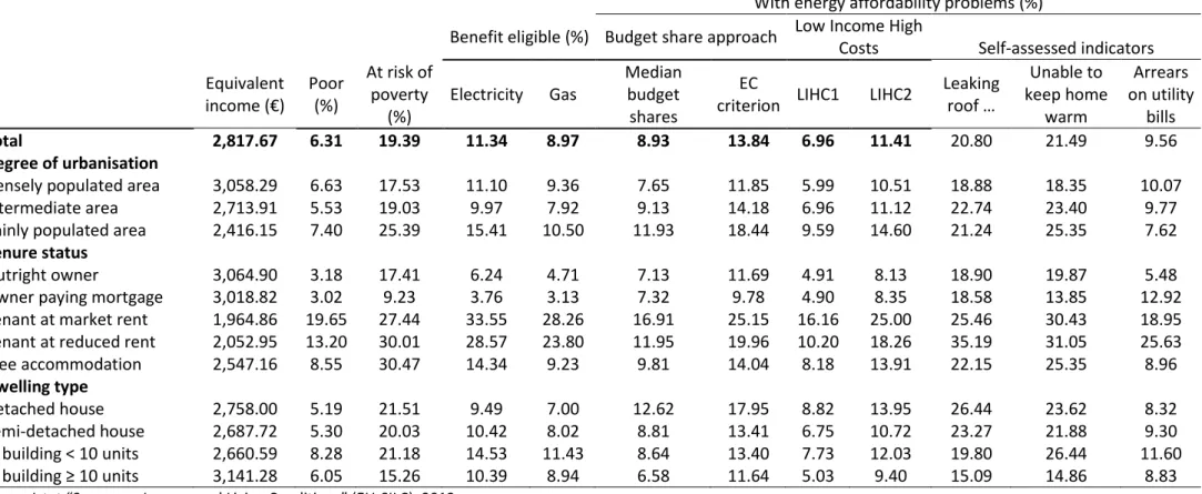
Table 4 continued: Average income, percentage of income poor, eligible households, and households with affordability problems. Equivalent income (euro per month): household income net

of taxes and contribution to the social security system, including imputed rents, divided by the equivalence scale used for the definition of the absolute poverty line. Poor: households whose adult equivalent income is below the absolute poverty line. At risk of poverty: households whose adult equivalent income is lower than 60% of median adult equivalent income. Median budget shares: median budget shares of the relatively poor, by household size and climatic classification of the area of residence. EC criterion: 2* Average expenditure / Average income, by household size and climatic classification of the area of residence. LIHC1: (Income – energy spending < EC relative poverty line) AND (energy budget share > median budget share). LIHC2: (Income < absolute poverty line) OR (energy budget share > median budget share).

With energy affordability problems (%) Benefit eligible (%) Budget share approach Low Income High

Costs Self-assessed indicators

Equivalent income (€) Poor (%) At risk of poverty (%) Electricity Gas Median budget shares EC

criterion LIHC1 LIHC2

Leaking roof … Unable to keep home warm Arrears on utility bills Total 2,817.67 6.31 19.39 11.34 8.97 8.93 13.84 6.96 11.41 20.80 21.49 9.56 Degree of urbanisation

Densely populated area 3,058.29 6.63 17.53 11.10 9.36 7.65 11.85 5.99 10.51 18.88 18.35 10.07

Intermediate area 2,713.91 5.53 19.03 9.97 7.92 9.13 14.18 6.96 11.12 22.74 23.40 9.77

Thinly populated area 2,416.15 7.40 25.39 15.41 10.50 11.93 18.44 9.59 14.60 21.24 25.35 7.62

Tenure status

Outright owner 3,064.90 3.18 17.41 6.24 4.71 7.13 11.69 4.91 8.13 18.90 19.87 5.48

Owner paying mortgage 3,018.82 3.02 9.23 3.76 3.13 7.32 9.78 4.90 8.35 18.58 13.85 12.92

Tenant at market rent 1,964.86 19.65 27.44 33.55 28.26 16.91 25.15 16.16 25.00 25.46 30.43 18.95 Tenant at reduced rent 2,052.95 13.20 30.01 28.57 23.80 11.95 19.96 10.20 18.26 35.19 31.05 25.63

Free accommodation 2,547.16 8.55 30.47 14.34 9.23 9.81 14.04 8.18 13.91 22.15 25.35 8.96 Dwelling type Detached house 2,758.00 5.19 21.51 9.49 7.00 12.62 17.95 8.82 13.95 26.44 23.62 8.32 Semi-detached house 2,687.72 5.30 20.03 10.42 8.02 8.81 13.41 6.75 10.72 23.27 21.88 9.30 In building < 10 units 2,660.59 8.28 21.18 14.53 11.43 8.64 13.40 7.73 12.03 19.80 26.44 11.60 In building ≥ 10 units 3,141.28 6.05 15.26 10.39 8.94 6.58 11.64 5.03 9.40 15.09 14.86 8.83 Source: Istat “Survey on Income and Living Conditions” (EU-SILC), 2012.

15

Considering the results in Table 4, we notice that, no matter the definition of energy affordability we adopt, low income categories are those with highest incidence of energy poverty. So, for instance, the “single parents” households are those with the lowest per capita disposable income (1,867.68 euro per month), result to be those with the highest percentage in absolute poverty and at risk of poverty (23.7% and 38.3% respectively) and also those affected by the highest incidence of energy poverty. In general, changing the definition of energy poverty or a component of its indicator has two major effects on the assessment of energy affordability. On the one hand, it can change significantly the level of energy poverty measured: going from the “objective” criterion LIHC1 to the “subjective” criterion relying on the self-assessment of being able to keep the home warm shift the incidence of energy poverty in the entire population from 7% to 21.5%. On the other hand, it can remarkably change the identification of the group of household most/least in need. For instance, according to the budget share approach if one takes the EC criterion as a threshold, one-person households are more in need than the households classified as “others with children”, but the conclusion is reversed if the critical threshold is the median budget share. The table provides illuminating evidence on how the choice of the instrument adopted to measure the phenomenon can have dramatic effects on the policy decisions, both in terms of assessment of its relevance and targeting of the intervention.

Although higher levels of energy poverty are typically associated with lower disposable income, the type of accommodation seems to play a major role in determining energy vulnerability. The second part of Table 4 highlights that detached houses have the poorest maintenance conditions, and that their inhabitants are more likely to have energy affordability problems, despite the fact that they are relatively well off. The high incidence of energy poverty among tenants is also potentially due to the combination of their low income together with the low energy efficiency of their houses. As the eligibility criterion is explicitly designed to target low-income households, we expect the percentage of eligible households to vary across groups together with the incidence of absolute poverty and the percentage of households at risk of poverty. The percentage of eligible households is always higher for the electricity benefit than for the gas one. This is particularly relevant in the southern regions and islands due to the geographical limitation of the gas distribution grid and the differences in gas consumption in areas with different climatic conditions.

16

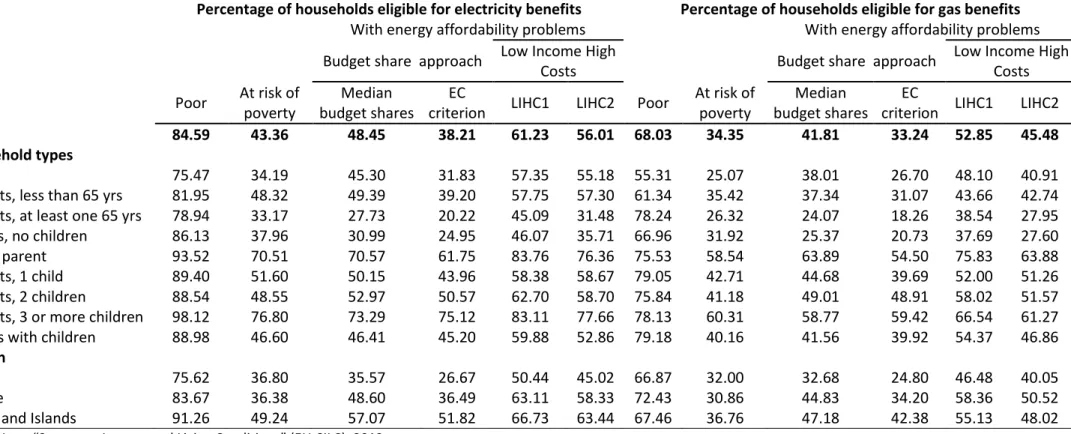
Table 5: Percentage of eligible households among poor households, households at risk of poverty and households with affordability problems. Poor: household whose adult equivalent income

is below the absolute poverty line. At risk of poverty: households whose adult equivalent income is lower than 60% of median adult equivalent income. Median budget shares: median budget shares of the relatively poor, by household size and climatic classification of the area of residence. EC criterion: 2* Average expenditure / Average income, by household size and climatic classification of the area of residence. LIHE1: (Income – energy spending < EC relative poverty line) AND (energy budget share > median budget share). LIHE2: (Income < absolute poverty line) OR (energy budget share > median budget share).

Percentage of households eligible for electricity benefits Percentage of households eligible for gas benefits

With energy affordability problems With energy affordability problems Budget share approach Low Income High

Costs Budget share approach

Low Income High Costs Poor At risk of poverty Median budget shares EC

criterion LIHC1 LIHC2 Poor

At risk of poverty

Median budget shares

EC

criterion LIHC1 LIHC2

Total 84.59 43.36 48.45 38.21 61.23 56.01 68.03 34.35 41.81 33.24 52.85 45.48

Household types

Single 75.47 34.19 45.30 31.83 57.35 55.18 55.31 25.07 38.01 26.70 48.10 40.91

2 adults, less than 65 yrs 81.95 48.32 49.39 39.20 57.75 57.30 61.34 35.42 37.34 31.07 43.66 42.74 2 adults, at least one 65 yrs 78.94 33.17 27.73 20.22 45.09 31.48 78.24 26.32 24.07 18.26 38.54 27.95 Others, no children 86.13 37.96 30.99 24.95 46.07 35.71 66.96 31.92 25.37 20.73 37.69 27.60

Single parent 93.52 70.51 70.57 61.75 83.76 76.36 75.53 58.54 63.89 54.50 75.83 63.88

2 adults, 1 child 89.40 51.60 50.15 43.96 58.38 58.67 79.05 42.71 44.68 39.69 52.00 51.26

2 adults, 2 children 88.54 48.55 52.97 50.57 62.70 58.70 75.84 41.18 49.01 48.91 58.02 51.57 2 adults, 3 or more children 98.12 76.80 73.29 75.12 83.11 77.66 78.13 60.31 58.77 59.42 66.54 61.27 Others with children 88.98 46.60 46.41 45.20 59.88 52.86 79.18 40.16 41.56 39.92 54.37 46.86

Region

North 75.62 36.80 35.57 26.67 50.44 45.02 66.87 32.00 32.68 24.80 46.48 40.05

Centre 83.67 36.38 48.60 36.49 63.11 58.33 72.43 30.86 44.83 34.20 58.36 50.52

South and Islands 91.26 49.24 57.07 51.82 66.73 63.44 67.46 36.76 47.18 42.38 55.13 48.02

17

Table 5 shows the percentage of eligible households among poor households, households at risk of poverty and households with affordability problems according to the budget share or the Low Income High Costs approaches. Among the absolute poor, we observe that about 15% of them are not eligible for the electricity benefits and 32% are not eligible for gas benefits. Among households at risk of poverty, only 43% are eligible for the electricity benefits and 34% for the gas ones.

Considering the energy poor households, we observe large changes in the eligibility rates as we change the definition of affordability. The eligibility rates are the lowest among the households classified as energy poor according to the budget share approach with the EC criterion threshold (38% for electricity and 33% for gas benefits), and the highest with the LIHC1 approach (61% for electricity and 53% for gas).

Eligibility rates vary remarkably across household types and area: for example, among households in absolute poverty, the eligibility rate for the electricity benefit is 75.5% for the one-person households and 98.1% for households with two adults and at least three children. Similarly, for given income or energy poverty conditions, the eligibility rates in southern regions are higher than in the rest of the country.

The fact that the eligibility criteria exclude a significant portion of households in need from the benefits is due to a combination of different reasons, three of which refer to the adoption of the Equivalent Economic Conditions Indicator (ISEE); in particular:

(i) the Equivalent Economic Conditions Indicator (ISEE), which is used to assess the financial resources of the households, refers to a definition of income that differs from the one considered by standard poverty analyses. In fact, the ISEE considers the gross household income together with an estimate of the income produced by real estate and financial wealth, while the poverty statistics refer to net household income including imputed rents due to primary residence ownership and social transfers. Accounting for home-ownership and the value of real estate tend to decrease the eligibility rates of homeowners, in particular in the Northern regions and large cities, where the values of the houses are considerably higher than in the rest of the country.

(ii) the Equivalent Economic Conditions Indicator (ISEE) is based on an equivalence scale that is slightly different from the one used for poverty definition. In particular, it attaches a relevant

18

weight to the presence of disabled individuals, single parents, presence of with children and occupational status, while the equivalence scale used for the poverty indicators considers only the size of the household and the age of its members. This can explain some of the differences in eligibility rates across different household types.

(iii) the threshold value of the Equivalent Economic Conditions Indicator (ISEE) does not vary with the region of residence, while the components of the absolute poverty line are region-specific, as they consider differences in prices, housing markets and heating needs. This generates different eligibility rates across the regions of the country.

(iv) the eligibility criteria do not depend on households' energy consumption; by design the policy is not particularly well suited to support consumers who face affordability problems despite their spending ability is above the subsistence level.

(v) in order to be eligible for the gas benefit, the households must be connected to the natural gas network, and this dramatically reduces eligibility among households living in areas not served by the gas distribution grid.

4.3 A focus on the eligibility for benefits

So far, we have studied the eligibility and the energy poverty rates by relying on simple descriptive statistics. Although informative, these tables do not allow us to disentangle the effects of the determinants that are at work at the same time. For instance, the difference across areas in the energy poverty rates may be simply due to the well-known differences in income across areas. In order to further investigate the main drivers of energy poverty and to evaluate to what extent the benefit policy adopted to support Italian vulnerable consumers in those market is able to target public resources to families in need, we resort to a multiple regression approach. Our goal is to show the key determinant of the probability of being energy poor and eligible for electricity benefits. Remind that electricity and gas benefits have the same income eligibility criterion, therefore if the household is eligible for the electricity benefit, it would be eligible also for gas benefit if it used natural gas. We analyse how the percentage of energy vulnerable households eligible for the energy benefits changes not only because of their ability to spend, but also depending on other characteristics, as family composition, occupational and tenure status.

19

We model the joint probability of being energy poor and eligible for the energy benefits by resorting to a bivariate probit model (see Cameron et al., 2005). We consider a household to be energy poor according to the Low Income High Cost criterion, in which:

 the “low income” condition is assessed referring to the absolute poverty line, and

 the “high cost” condition is satisfied if the incidence of energy spending on income is

higher than the median energy budget shares of the (relatively) poor households of similar size living in the same climatic area.

The probability of being energy poor is therefore a function of income level and energy spending. For given level of income and spending, the energy poverty status is affected also by household composition, area of residence, housing conditions and type of fuel used for heating.

Household’s income is – in principle – the only determinant of the eligibility. In practice, this is not actually the case, because eligibility depends on an estimate of income from real estate and financial assets, which are not included in the standard definition of disposable income. The latter is instead routinely used in any household welfare analysis, both in Italy and in the European Union. This implies that the type and location of the accommodation and the tenure status affect the eligibility of the households, because of their impact on the real estate wealth.

Furthermore, the way the eligibility criterion accounts for family composition and occupational status differs from the standard adjustment via equivalent scale. We therefore consider household composition and occupational status as possible determinants of the eligibility status, also once controlled for household adult equivalent disposable income.

Overall, only the variables describing the type of fuels used and the incidence of energy spending on household disposable income affect exclusively the energy poverty status and not the eligibility one. We therefore specify the following multivariate model:



1 1





2 2



h h h h h h h

EnPov 1 x z  u Eli 1 x  u

where EnPovh is a dummy variable equal 1 if household h is energy poor, zero otherwise; Elih is a

dummy variable for the eligibility status; 1(.) is an indicator function that equals one if the

condition in parentheses hold true and zero otherwise; xh is vector of household and

20

the type of fuels used by the households and the incidence of energy expenditure on household

income. The random components (uh1,uh2) are jointly normally distributed, independently and

identically distributed with unitary variance and correlation . The unknown parameters



   1, 2, ,



are estimated via maximum likelihood.

As the bivariate probit model is highly non-linear, it is easier to assess the effect of the covariates on the outcomes by looking at the marginal effects of x and z on the probability of being energy poor and eligible, rather than simply looking at the estimated parameters. We thus consider the marginal effect on the probability of being energy poor, that is Pr



EnPov_h|x z_h, _h



/x_h and





Pr EnPov_h|x z_h, _h / z_h

  , the probability of being eligible for the energy benefits





Pr Eli_h|x_h / x_h

  ; and of the probability of being eligible, given that the household is energy

poor, Pr



Eli_h|EnPov_h 1,x z_h, _h



/x_h and Pr



Eli_h|EnPov_h1,x z_h, _h



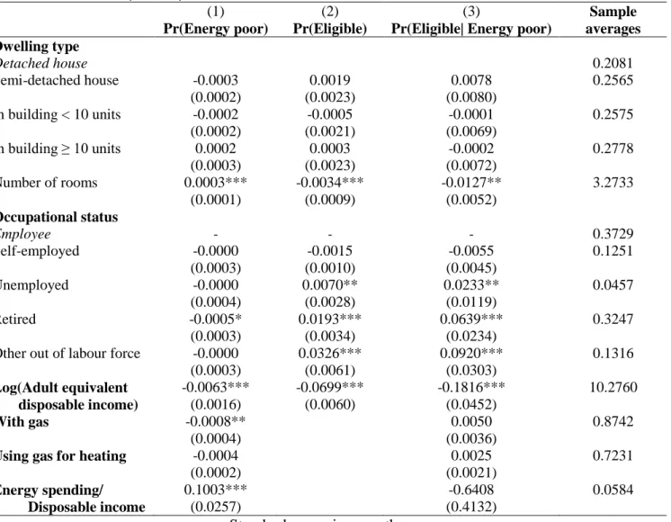
/z_h.

Table 6 shows estimated marginal effects computed at the average values of the covariates. As expected, an increase in income - Log(Adult equivalent disposable income) - reduces the probability of being energy poor and eligible for the benefits. Vice-versa, keeping income and the other characteristics constants, an increase in the energy budget shares raises the probability of being energy poor. Family composition plays a role in both marginal probabilities, but usually with opposite signs: at the mean values, the single-person household is the one least likely to be energy poor according to the LICH2 criterion, but it is the type of household most likely to be eligible for benefits, together with single parents. The conditional probability





Pr Eli_h|EnPov_h1,x z_h, _h confirms that – at the average values – the probability of a single-person household to be eligible is the highest.

There are significant territorial differences, also once controlled for compositional and income effects. The differences between homeowners and tenants are irrelevant for energy poverty, once income and other characteristics have been accounted for, while they persist as important determinants for eligibility: at the average values, the probability to be eligible for electricity benefits among the energy poor is about 13 percentage points higher for tenants with respect to outright homeowners.

21

Table 6: Marginal effects on the probability of being energy poor, eligible for energy benefits and eligible given that one is energy

poor. Marginal effects computed at the mean values of the explanatory variables. Standard errors in parentheses, in italics

reference option for qualitative variables.

(1) (2) (3) Sample

Pr(Energy poor) Pr(Eligible) Pr(Eligible| Energy poor) averages

Household types

Without children

Single - - - 0.3030

2 adults, 0.0007** -0.0120*** -0.0495** 0.1037

both younger than 65 yrs (0.0003) (0.0030) (0.0215)

2 adults, 0.0004** -0.0047 -0.0235 0.1490

at least one over 65 yrs (0.0002) (0.0031) (0.0145)

Others 0.0029*** -0.0133*** -0.0580** 0.1266 (0.0010) (0.0028) (0.0254) With children Single parent 0.0030* 0.0144* 0.0135 0.0309 (0.0017) (0.0078) (0.0186) 2 adults, 1 child 0.0007** -0.0134*** -0.0548** 0.1057 (0.0003) (0.0028) (0.0229) 2 adults, 2 children 0.0023*** -0.0120*** -0.0534** 0.1055 (0.0008) (0.0028) (0.0235) 2 adults, 3 or 0.0049** 0.0302** 0.0421 0.0213 more children (0.0022) (0.0124) (0.0257) Others 0.0095*** -0.0083** -0.0483** 0.0543 (0.0031) (0.0037) (0.0239) Area of residence North - - - 0.4828 Centre 0.0015*** 0.0037** 0.0051 0.1989 (0.0005) (0.0018) (0.0057)

South and Islands 0.0008** 0.0131*** 0.0342*** 0.3183

(0.0003) (0.0027) (0.0113)

Degree of urbanization

Densely populated area - - - 0.4391

Intermediate area -0.0003 0.0036** 0.0134* 0.3993

(0.0002) (0.0016) (0.0070)

Thinly populated area -0.0005** 0.0118*** 0.0403** 0.1615

(0.0002) (0.0030) (0.0160)

Tenure status

Outright owner - - - 0.6054

Owner paying mortgage 0.0001 -0.0021 -0.0080 0.1371

(0.0003) (0.0016) (0.0062)

Tenant at market rent 0.0001 0.0579*** 0.1454*** 0.1335

(0.0002) (0.0079) (0.0399)

Tenant at reduced rent -0.0003 0.0470*** 0.1310*** 0.0485

(0.0002) (0.0090) (0.0415)

Free accommodation -0.0000 0.0092** 0.0293** 0.0755

(0.0003) (0.0036) (0.0143)

Standard errors in parentheses *** p<0.01, ** p<0.05, * p<0.1

22

Table 6 continued. Marginal effects on probability of being energy poor, eligible for energy benefits and eligible given that one is energy poor. Marginal effects computed at the mean values of the explanatory variables. Standard errors in parentheses, in

italics reference option for qualitative variables.

(1) (2) (3) Sample

Pr(Energy poor) Pr(Eligible) Pr(Eligible| Energy poor) averages

Dwelling type Detached house 0.2081 Semi-detached house -0.0003 0.0019 0.0078 0.2565 (0.0002) (0.0023) (0.0080) In building < 10 units -0.0002 -0.0005 -0.0001 0.2575 (0.0002) (0.0021) (0.0069) In building ≥ 10 units 0.0002 0.0003 -0.0002 0.2778 (0.0003) (0.0023) (0.0072) Number of rooms 0.0003*** -0.0034*** -0.0127** 3.2733 (0.0001) (0.0009) (0.0052) Occupational status Employee - - - 0.3729 Self-employed -0.0000 -0.0015 -0.0055 0.1251 (0.0003) (0.0010) (0.0045) Unemployed -0.0000 0.0070** 0.0233** 0.0457 (0.0004) (0.0028) (0.0119) Retired -0.0005* 0.0193*** 0.0639*** 0.3247 (0.0003) (0.0034) (0.0234)

Other out of labour force -0.0000 0.0326*** 0.0920*** 0.1316

(0.0003) (0.0061) (0.0303)

Log(Adult equivalent -0.0063*** -0.0699*** -0.1816*** 10.2760

disposable income) (0.0016) (0.0060) (0.0452)

With gas -0.0008** 0.0050 0.8742

(0.0004) (0.0036)

Using gas for heating -0.0004 0.0025 0.7231

(0.0002) (0.0021)

Energy spending/ 0.1003*** -0.6408 0.0584

Disposable income (0.0257) (0.4132)

Standard errors in parentheses *** p<0.01, ** p<0.05, * p<0.1

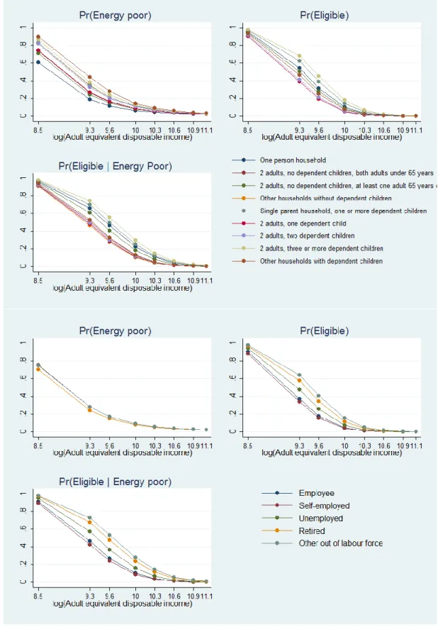
As the estimated model is non-linear, the differences between groups are not constant, and they depend on the value of all the variables at play. In particular, given the skewness of the income distribution, and the attention to the low-income households, it is worth considering how the differences between groups vary with income. In Figures 1 and 2 we plot the three probabilities





Pr EnPov_h|x z_h, _h , Pr



Eli_h|x_h



and Pr



Eli_h|EnPov_h1,x z_h, _h



for different level of income and by different subgroups of households. More specifically, we compute the probabilities at the 1st, 5th, 10th, 25th, 50th, 75th, 90th and 95th percentiles of adult equivalent disposable income, keeping all other variables at their observed values. We expect the probabilities to be energy poor and eligible to be the highest for low values of income and drop to zero for affluent households. The speed at which this happens may differ between household groups.

23

Figure 1 shows the predicted probabilities for different level of income, by household type and occupational status. Looking at the probability of being energy poor, it is possible to observe how the predicted probability is different across different household types for low level of income and how the difference vanishes as income increases, becoming negligible around the median value of income. For the eligibility rate, the picture is rather different: there are no differences between

types for very low levels of income (1st percentile), where all households are predicted to be

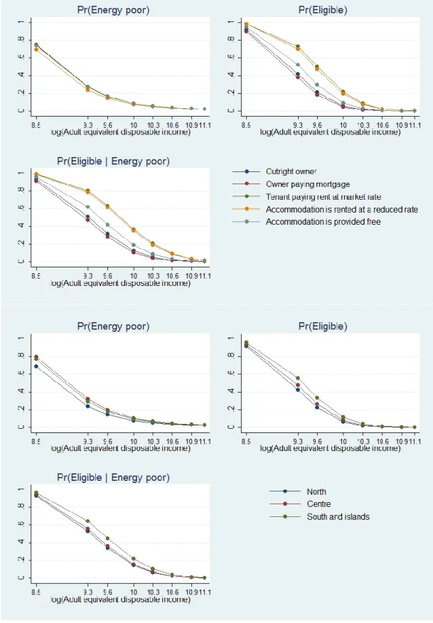
eligible, then the differences widens reaching their maximum around the fifth percentile, and then decreases. Large differences in the eligibility probability are depicted also between different occupational status (second panel of Figure 1) and housing tenure (first panel of Figure 2), which instead do not affect energy poverty. The latter result is apparently in sharp contrast with the descriptive evidence provided in Table 4, where a considerably higher incidence of energy poverty is reported for tenants. The use of a multiple regression strategy allows us to say that such difference is mainly due to income differences between tenants and homeowners, that is, when tenants and homeowners of similar income level are confronted, there is no relevant difference in their probability of being energy poor.

The regression analysis confirms the presence of a persistent difference in the regional eligibility rates: the second panel of Figure 2 shows that among energy poor households with adult

equivalent income around the 5th percentile, the eligibility rate in the Southern regions is about

65%, 10 percentage points higher than in the Centre and North areas. As previously explained, this can be due to the heterogeneity in price levels, housing values and different labour market participation rates.

Overall, the graphs make evident that, ceteris paribus, the eligibility criterion does not guarantee equal opportunity of access to the benefits, but it rather privileges the households with children, those households whose head is out of labour force, the tenants and the resident in the Southern regions.

24

Figure 1: Predicted probability of being energy poor and eligible for energy benefits as function of adult equivalent disposable income, by household type and occupational status of the head of the households. Predicted values are computed at 1st, 5th, 10th, 25th, 50th, 75th, 90th and 95th percentiles of adult equivalent disposable income, keeping all other variables at their observed values.

25

Figure 2: Predicted probability of being energy poor and eligible for energy benefits as function of adult equivalent disposable income, by tenure status and area of residence. Predicted values are computed at 1st, 5th, 10th, 25th, 50th, 75th, 90th and 95th percentiles of adult equivalent disposable income, keeping all other variables at their observed values.

26

5

Conclusions

Alternative indices of affordability in energy consumption focus on different aspects of the energy poverty; any sensible indicator should combine information on households income and the achievement of a minimum standard of quality of life, also considering under-spending as a potential cause of deprivation. The actual implementation of these principles has to deal with the nature of the available data and it needs to be complemented by a precise analysis of the determinants of the affordability problem.

In this chapter we have shortly presented alternative indices of affordability in energy consumption (i.e. budget share approach and Low Income High Cost approach) and provided their measurement for Italy in 2012. Our results highlight the different pictures about Italian vulnerable consumers in energy markets from adopting the alternative indices.

We then describe the Italian scheme of energy benefits which consists of a lump-sum contribution on the vulnerable consumers’ bills. The amount of the both electricity and gas benefits refers to the number of household components; the amount is for both independent of the household’s actual consumption; and the gas benefit depends on the index about climatic conditions of the area of the households’ residence. The policy provides a limited benefit to a potentially large number of beneficiaries: in 2012, the amount of the electricity benefit ranged between 63 euro per year for a couple and 139 euro for a household with more than 4 members (plus 10% VAT); the amount of the gas benefit ranged from 85 euro for a household with less than 5 members living in the warmest part of the county, to 318 euro for a household with at least 5 members living in the coldest areas (plus 21% VAT).

Our empirical results show the changes in the eligibility rates, according to the alternative definition of affordability in energy consumption. We also discuss several reasons why the adopted eligibility criteria excludes a significant proportion of Italian households in need from the benefits.

Finally, we set a multiple regression model to investigate the key determinant of the probability of being energy poor and eligible for energy benefits. As expected, an increase in income reduces the probability of being energy poor and eligible for energy benefits; keeping income and the other characteristics constants, an increase in the energy budget shares raises the probability of being energy poor. Family composition plays a role in both marginal probabilities, but usually with opposite signs: at the mean values, the single-person household is the one least likely to be energy poor according to the LICH2 criterion, but it is the type of household most likely to be eligible for benefits, together with single parents. At the average values, the probability of a single-person household to be eligible is the highest. There are significant territorial differences, also once controlled for compositional and income effects. All in all, our analysis shows that, ceteris paribus, the eligibility criterion does not guarantee equal opportunity of access to the benefits, but it rather privileges the households with children, those households whose head is unemployed, the tenants and the resident in the Southern regions.

27

References

Cameron, A. Colin, and Pravin K. Trivedi. Microeconometrics: methods and applications. Cambridge university press, 2005.

Chaplin, R. and A. Freeman (1999), "Towards an Accurate Description of Affordability", Urban Studies, 36 (11), pp. 1949-57.

DEFRA (2001). The UK Fuel Poverty Strategy - 1st Annual Progress Report 2003, http://www.dti.gov.uk/energy/consumers/fuel_poverty/index.shtml

DEFRA (2007), The UK Fuel Poverty Strategy, First Annual Progress Report 2006,

http://webarchive.nationalarchives.gov.uk/+/http://www.berr.gov.uk/files/file29688.pdf

Fankhauser, S. and S. Tepic (2007) “Can poor consumers pay for energy and water? An affordability analysis for transition countries”, Energy Policy, 32(2), pp. 1038-1049.

Hancock, K. E. (1993), `Can Pay? Won't Pay?' or Economic Principles of `Affordability’, Urban Studies, 30(1), pp. 127-145.

Healy, J. (2001), Home Sweet Home? Assessing Housing Conditions and Fuel Poverty in Europe, ERSR WP 01/13, University College Dublin.

Hills, J. (2012): Getting the measure of fuel poverty. Final Report of the Fuel Poverty Review.

Download from: http://sticerd.lse.ac.uk/dps/case/cr/CASEreport72.pdf

ISTAT (2004), La povertà assoluta: informazioni sulla metodologia di stima, Approfondimenti – Famiglia e società, Roma: ISTAT

ISTAT (2009), La misura della povertà assoluta, Metodi e norme n. 39, 2009.

Miniaci, R., C. Scarpa, Valbonesi, P. (2008a), Measuring the affordability of public utility services in Italy, Giornale degli Economisti ed Annali di Economia, pp.185-230.

Miniaci, R., C. Scarpa, Valbonesi, P. (2008b), Distributional effects of the price reforms in the Italian utility markets, Fiscal Studies, 29/1, pp.135-163.

Miniaci, R., C. Scarpa, Valbonesi, P. (2014a), Fuel poverty and the energy system: the Italian case, IEFE Working Paper n.66.Sen, A. (1976): “Poverty: an ordinal approach to measurement”, Econometrica, 44, pp. 219-31.

Sefton, T. (2002), Targeting Fuel Poverty in England: is the government getting warm?, Fiscal Studies, 23/3, pp. 369-399.

Sefton, T. and J., Chesshire, (2005), Peer Review of the Methodology for Calculating the Number of Households in Fuel Poverty in England. Final Report to DTI and DEFRA.,

28

Stone, M. E. (1993), Shelter Poverty: New Ideas on Housing Affordability, Philadelphia: Temple University Press.

Thalmann, P. (2003), "House poor or simply poor?", Journal of Housing Economics, 12, pp. 219-317.

Waddams Price, C. , Brazier, K. and W. Wang (2012): Objective and subjective measures of fuel

poverty, Energy Policy, 49, pp. 33–39

View publication stats View publication stats