POLITECNICO DI MILANO
MSc in Computer Science and Engineering Scuola di Ingegneria Industriale e dell’Informazione Dipartimento di Elettronica, Informazione e Bioingegneria
AN EXPERIMENT IN AUTONOMOUS
NAVIGATION FOR A SECURITY
ROBOT
AI & R LabLaboratorio di Intelligenza Artificiale e Robotica del Politecnico di Milano
Supervisor: Prof. Matteo Matteucci Co-supervisor: Ing. Gianluca Bardaro
Master Graduation Thesis by: Fabio Santi Venuto, Student ID 837644
Abstract
One of the most useful purpose in autonomous robots is to substitute for human activity in the so called Dirty, Dangerous, Dull (DDD) tasks. The Ra.Ro platform, developed by NuZoo, is designed to work as a security robot, able to patrol, detect anomalies, and eventually send alarms to a cen-tralized station. This platform is has to be adapted to different purposes and customized for each client, but in most of cases an autonomous navigation is required. The aim of this thesis is to propose a mapping and localization system to avoid the well-known odometry drifting problem and allow for long term autonomous navigation the Ra.Ro. platform. In particular, the robot moves in an indoor environment, challenging because of the lack of any global positioning sensor such as GPS in outdoor. The odometry system provided by the wheel encoders is not precise enough and very sensitive to errors, thus it is important to fuse the information retrieved by multiple sen-sors such as IMU, LIDAR and a camera used to recognize specific markers in order to compensate for odometry drifting.
The final results, testing the robot in real world scenarios, are quite sat-isfying, allowing finally the robot to move autonomously in an environment previously mapped.
Sommario
I robot autonomi nel ruolo di guardia di sicurezza non sono ancora comuni. Una guardia efficiente deve essere abile nell’individuare persone non autor-izzate o qualsiasi altra cosa che non vada bene. Deve essere reattiva, veloce e ovviamente difficile da battere. Probabilmente la tecnologia attuale `e pre-matura, ma la piattaforma Ra.Ro. `e molto semplice da adattare a scenari differenti, a seconda delle richieste dei clienti. Essendo un robot basato su una meccanica Skid-steering, ha senza dubbio l’abilit`a di muoversi autono-mamente nell’ambiente, a prescindere dalla sua finalit`a.
La navigazione “autonoma” del Ra.Ro. commercializzato finora con-siste nel seguire delle linee colorate incollate o dipinte sul pavimento e/o seguire delle indicazioni date da dei marker appartenenti ad uno specifico set e riconosciuti dalle telecamere installate. I problemi di questi approcci sono faclimente individuabili. Prima di tutto, in determinati luoghi, non `e desiderabile avere il pavimento rovinato da linee incollate o dipinte, mentre all’aperto `e praticamente impossibile disegnarle o incollarle. Inoltre diverse condizioni luminose possono condizionare il riconoscimento del colore delle linee. Possiamo avere problemi simili quando abbiamo a che fare con i marker, che hanno bisogno di essere appesi su muri o altri tipi di strutture stabili. Se il robot usa le linee e i marker per pattugliare un edificio per ra-gioni di sicurezza, sarebbe facile per un malintenzionato coprire, cancellare o staccarli, facendo perdere il robot in pochi secondi.
Ringraziamenti
Poche parole, anche perch´e di pi`u non me ne verrebbero. Sicuramente i miei genitori sono le persone a cui vanno i miei pi`u sentiti ringraziamenti. Sar`a banale dirlo, ma senza di loro e il loro supporto non sarei qui. Mio padre dice sempre che “La libert`a `e avere le possibilit`a” e loro sono stati in grado di darmi la libert`a necessaria e sono sicuro che continueranno a farlo. Grazie a mia sorella, Valeria, che mi sa capire e che nel momento del bisogno c’`e sempre.
Un ringraziamento speciale alla mia ragazza, Desy, che mi ha accompa-gnato durante questo lungo percorso, dal primo giorno di universit`a, fino all’ultimo, aggiungendo un pizzico di amore che ha reso la strada da percor-rere pi`u piacevole.
Grazie agli amici di una vita, i miei amici pievesi (ed ex pievesi); Ori, Andre, Mane e Gabry, e i nuotatori in pensione; Paolo, Gi`o, Andreino e Teo. Di cuore a tutti un abbraccio. Insostituibili.
Grazie a mio cugino, Alessandro, che da quando `e tornato in Italia mi ha riavvicinato ad un pezzo di cultura: i videogiochi :) Forse ora avremo pi`u tempo per giocare a Overwatch con Alberto.
Grazie agli amici incontrati in universit`a, in particolare ai ragazzi dell’AirLab, Ewerton, Enrico, Davide e Dave, Teo e Luca e tutti coloro che sono passati da l`ı. Hanno reso l’ambiente di lavoro davvero speciale e il loro supporto morale e tecnico `e stato fondamentale.
Infine, ma non ultimi, grazie ai professori, in particolare il mio relatore, Matteucci, una persona che mille ne pensa e duemila ne fa -letteralmente-e Gianluca ch-letteralmente-e mi hanno fatto capir-letteralmente-e un po’ di pi`u cosa vuol dire essere un ingegnere informatico.
Grazie,
Fabio
Contents
Abstract 5 Sommario 7 Ringraziamenti 9 1 Introduction 15 1.1 Thesis contribution . . . 161.2 Structure of the thesis . . . 16
2 The Ra.Ro. platform 19 2.1 Ra. Ro. Hardware . . . 19
2.2 Ra.Ro. Software . . . 20
2.2.1 ROS topics . . . 21
2.2.2 Built-in navigation . . . 23
3 Background knowledge 25 3.1 State estimation . . . 25
3.1.1 Baysian state estimation . . . 26
3.1.2 Graph-based State Estimation . . . 28
3.2 Odometry estimation . . . 29
3.2.1 Generic odometry . . . 29
3.2.2 Differential drive odometry . . . 31
3.2.3 Skid-steering odometry . . . 34
3.3 Sensor fusion framework . . . 38
3.3.1 ROAMFREE . . . 38
3.4 Simultaneous Localization and Mapping . . . 43
3.4.1 Gmapping . . . 46
3.4.2 Cartographer . . . 47
3.5 Localization . . . 48
3.5.1 Adaptive Monte Carlo Localization (AMCL) . . . 50
3.6 A note on ROS reference system . . . 50
4 A new navigation system for the Ra.Ro. 53 4.1 Navigation system overview . . . 53
4.2 Sensor fusion and odmetry estimation . . . 55
4.2.1 Custom odometry . . . 56
4.2.2 ROAMFREE module . . . 59
4.3 SLAM module . . . 64
4.4 Autonomous navigation module . . . 65
5 Experiments 67 5.1 Setup description . . . 67
5.2 Odometry experiments . . . 69
5.2.1 Custom odometry . . . 70
5.2.2 ROAMFREE odometry . . . 71
5.2.3 ROAMFREE with markers odometry . . . 72
5.3 Mapping experiments . . . 74
5.3.1 Mapping with custom odometry . . . 74
5.3.2 Mapping with ROAMFREE odometry . . . 75
5.3.3 Mapping with ROAMFREE odometry and markers . 76 5.4 Navigation experiments . . . 76
6 Conclusion and Future Work 79 A About ROS and the TF library 81 A.1 ROS Filesystem Level . . . 82
A.2 ROS Computation Graph Level . . . 82
A.3 The TF library . . . 84
B Sensors specifications 87 B.1 LSM303D Ultra compact high performance e-compass: 3D accelerome-ter and 3D magnetomeaccelerome-ter module . . . 88
B.2 L3GD20H MEMS motion sensor: three-axis digital output gyroscope . . 89
B.3 Hokuyo URG-04LX-UG01 Scanning Laser Rangefinder . . . . 90
List of Figures
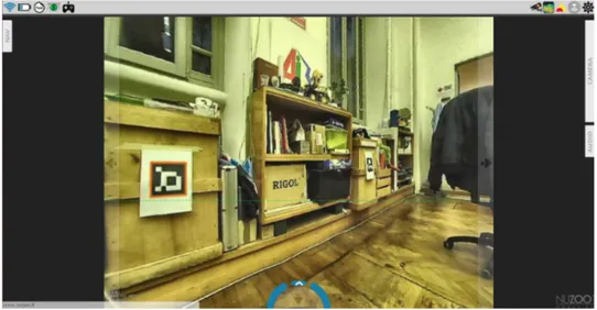
2.1 Three Ra.Ro. views . . . 20 2.2 NuZoo web interface. The recognized marker is orange
bor-dered. . . 21 2.3 Ra.Ro. photograph from NuZoo website . . . 23
3.1 A factor-graph for the product fA(x1)fB(x2)fC(x1, x2, x3)fD(x3, x4)fE(x3, x5). 28
3.2 Different integration methods results . . . 30 3.3 Commercial differential drive robots . . . 32 3.4 Differential drive kinematics . . . 33 3.5 Differential drive robot motion from pose (x, y, θ) to (x0, y0, θ0) 34 3.6 Ra.Ro. wheels . . . 35 3.7 Skid-steering platform . . . 36 3.8 Geometric equivalence between the wheeled skid-steering robot
and the ideal differential drive robot . . . 37 3.9 An instance of the pose tracking factor graph with four pose
vertices ΓWO(t) (circles), odometry edges eODO(triangles), two shared calibration parameters vertices kθ and kv (squares), two GPS edges eGP S and the GPS displacement parameter S(O)GP S . . . 40 3.10 ROAMFREE estimation schema . . . 42 3.11 The image represents the topics subscribed and published by
the mapping node, independently of the exact mapping sys-tem used . . . 45 3.12 The tree frame representation. . . 51
4.1 The ROS standard navigation stack schema . . . 54
4.2 Gyroscope measurement during two different time spans. The time difference is about 550 seconds and we can se how the bias change from an image to another. The represented mea-surements are raw data from gyroscope. We can see from the images comparison a difference of about 75. Considering that the LSB represents 17.5 mdps, this difference means that
exists a bias variation of 75 × 17.5mdps= 1.275dps. . . 58
4.3 An OptiTrack marker . . . 61
4.4 Different marker frame measurement passed to ROAMFREE. The ones blue highlated are the tranformation required and composed, the orange ones are the resulting transforamations 62 4.5 The tree frame representation, with node explanations . . . . 65
5.1 An approximate hand drown ground truth of the path made by the robot . . . 69
5.2 The resulting path generated with the custom odometry . . . 70
5.3 The resulting path generated with the ROAMFREE odome-try, without markers . . . 71
5.4 The resulting path generated with ROAMFREE odometry and markers . . . 73
5.5 Map generated using Cartographer. The long corridors result to be too short and the borders does not match properly. . . 74
5.6 The resulting map generated with the custom odometry . . . 75
5.7 The resulting map generated with the ROAMFREE odome-try without markers . . . 76
5.8 The resulting map generated with the ROAMFREE odome-try with markers . . . 77
5.9 The rviz visualization of the local and global costmaps . . . 78
A.1 The ROS Computations Graph . . . 84
A.2 A representation of a robot with several frames. . . 85
B.1 LSM303D module . . . 88
B.2 L3GD20H module . . . 89
Chapter 1
Introduction
“Narrator: Deep in the Caribbean, Scabb Island.
Guybrush: ...So I bust into the church and say, “Now you’re in for it, you bilious bag of barnacle bait!”... and then LeChuck cries, “Guybruysh! Have mercy! I can’t take it anymore!”
Fink: I think how he must have felt.
Bart: Yeah, if I hear this story one more time, I’m gonna be crying myself.” Monkey Island 2: LeChuck’s revenge
Autonomous robots as security guardian are not yet common. An efficient guard must be very smart in detecting unauthorized people or anything else wrong. It must be reactive, fast and of course hard to be defeated. Probably the current technology is premature to perform this task, but the Ra.Ro. platform is very easy to be adapted to different scenarios, according to the customers’ requests. Being a skid-steering based robot, it has certainly the ability to move autonomously in the environment, regardless of its high-level purpose.
Until now, the “autonomous” navigation of the commercialized Ra.Ro.s consists in following colored lines sticked or painted on the floor and/or following indications given by markers belonging to a specific set and rec-ognized by the installed cameras. The issues of these approaches are easy to identify. First of all, in some locations it is not desirable to have the floor ruined by sticked or painted lines while in outdoor environments it is almost impossible to draw or stick them. Moreover, different light condi-tions can affect the line color detection. We can have a similar issue when dealing with markers, which need to be hanged on walls or on similar stable structures. If the robot uses the lines and markers to patrol a building for security reasons, it will be quite easy for an malitious person to cover, delete or detach them, getting the robot lost in seconds.
1.1
Thesis contribution
The Ra.Ro. platform is already equipped with different sensors such as IMU (gyroscope, accelerometer and magnetometer), cameras and a LIDAR, but they were not used as much as they could be potentially done, especially these are not used for navigation.
This thesis proposes a multi-sensor navigation system based on the ROAM-FREE framework, a system that provides a multi-sensor fusion tools to im-prove the odometry estimation using the information provided by different sensors. We used the wheel encoders, gyroscope, accelerometer and, for a better result, visual markers as landmarks. Then, using the improved odometries, we generated and compared different maps using mostly the gmapping framework. Subsequently we set up the autonomous navigation system using the move base framework with AMCL and we tested the whole navigation stack in our indoor environments.
1.2
Structure of the thesis
The thesis is structured as follows:
• In Chapter 2 we describe the Ra.Ro. platform. In particular in Section 2.1 we introduce the hardware components which include the sensors provided with the robot. In Section 2.2 we introduce the robot built in software environment. In particular we describe the ROS topics used by the robot and the built in navigation systems in the following subsections.
• In Chapter 3 we provide the background knowledge needed to deeply understand in what our project consists. In particular, Section 3.1 introduces the most common state estimation approaches. Then, in Section 3.2, we focus on odometry estimation methods. Subsequently, in Section 3.3 we introduce the sensor fusion approaches we applied in this thesis, in particular we will introduce a custom odometry genera-tion method and the ROAMFREE framework. The following Secgenera-tion 3.4 is about SLAM, simultaneous localization and mapping, and two of the most popular ROS mapping systems. In Section 3.5 we describe the AMCL localization algorithm. We conclude with a note about the ROS reference system convention, in Section 3.6
• In Chapter 4 we describe our contribution, starting with the navigation system overview in Section 4.1. Then, in Section 4.2 we describe the
detail about the odometry estimation implementation and the sensor fusion framework applied. In Section 4.3 we explain how we used the mapping module.
• In Chapter 5, after a brief set up introduction in Section 5.1, we de-scribe the most significant experiment we make and the resulting out-put. In particular, we describe experiments about odometry estima-tion, in section 5.2, about mapping, in Section 5.3, and we provide a brief discussion about localization and autonomous navigation in section 5.4
• Finally in Chapter 6 we write about our conclusion, the main chal-lenges we had to deal with, and our suggestion about future works on this topic.
Chapter 2
The Ra.Ro. platform
“Guybrush: My name’s Guybrush Threepwood. I’m new in town
Pirate: Guybrush Threepwood? That’s the stupidest name I’ve ever heard! Guybrush: Well, what’s YOUR name?
Pirate: My name is Mancomb Seepgood.”
The Secret of Monkey Island
In this chapter we introduce the Ra.Ro. platform. Ra.Ro. stands for Ranger Robot, that is to say that its main purpose is to work as a security guard, able to patrol parkings, supermarkets and so on. However, the producer company, NuZoo offers the possibility of customizing the platform to meet different requests. It has already been adapted by the producer company for other different purposes, usually starting from its simpler version, code name Geko, which is very similar to Ra.Ro. except for the cameras, which are attached directly to the robot basis.
In the following paragraphs we focus on the version we have worked on, introducing its hardware and software suite. [1]
2.1
Ra. Ro. Hardware
Ra.Ro. is a skid steer drive robot. The basis is 460 mm x 540 mm and it is 270 mm tall. The robot reaches 750 mm including the cameras support. It is equipped with four wheels driven by two 50W DC motors, set in the middle of the two sides of the robot. Each motor drives a front and a rear wheel connected with two transmission belts.
The robot is equipped with a 9 axis IMU composed by a LSM303D module (3 axis magnetometer and 3 axis accelerometer) and a L3GD20H (3 axis gyroscope). The IMU is managed by a R2P board by Nova Labs [2]. A
Figure 2.1: Three Ra.Ro. views
Hokuyo Laser Scanner is included inside the robot body and allows a 170◦ view by projecting rays trough a 160 mm wide and 20 mm high body slit.
Inside the “head” of the Ra.Ro. are two HD cameras: a surveillance camera, which rotates according to the head itself and a navigation camera, which can, in addition, rotate around a horizontal axis. Vision into the darkness is guaranteed by two led flashlights. We can see in Figure 2.1 three Ra.Ro. views in which is possible to notice the two cameras, one flashlight inside the head, one near the basis and the body slit at the bottom, from which infrared laser rays are projected.
The core of the robot is an INTEL NUC built with an i5-5250U 64bit CPU, DDR3 4 GB RAM and SSD 60GB as a hard drive support. A Wi-Fi module is used to connect the robot to wireless nets or to convert it into an access point, in case of accessible net unavailability or first net setup. Ra.Ro. is able to recharge itself in a semi-autonomous way through a wide contacts-pins matching with its recharging station. In case of needs, a wired connection is also available to recharge the robot.
2.2
Ra.Ro. Software
The operative system currently installed on the NUC is Ubuntu 14.04 LTS, and all the robot features are managed by ROS Indigo. The provided ROS workspace includes most of the nodes and topics needed to start our work. In particular, we have nodes responsible for publishing sensors data, such as
Figure 2.2: NuZoo web interface. The recognized marker is orange bordered.
encoders, IMU, camera vision, laser scans and markers. Moreover, we have the nodes used to control the robot through the command velocity topics, via joy-pad or via browser interface. The browser interface itself is also a useful piece of software, which allows the user to see the images provided by the two cameras, the recognized marker, and to manage the various minor functionalities such as speakers, lights and so on. In Figure 2.2 we can see the camera view form the browser interface. When a marker is recognized, like in this case, an orange border is overlapped around the marker, in the camera view.
2.2.1 ROS topics
In this section we describe the most relevant, to our purposes, ROS topics published and/or subscribed by the previously implemented nodes. They allow the ROS system to communicate both with sensors and actuators, by reading outputs and sending commands respectively. The topics are introduced with the name and the message type used.
• /r2p/encoder l and /r2p/encoder r, [std msgs/Float32]:
These topics, and all of the following ones which have a name starting with r2p/, are published by the r2p board, which manages most of the sensors. In particular, these topics publish as messages the number of ticks per second done by the left wheels (r2p/encoder l) and the right ones (r2p/encoder r). Every tick corresponds to a portion of spun wheel.
• /r2p/imu raw, [r2p msgs/ImuRaw]:
This topic contains the raw messages from the IMU, including gy-roscope, accelerometer and magnetometer. The r2p msgs/ImuRaw is a custom message type built by three tridimensional vectors: angular velocity, linear acceleration and magnetic field. The names are self-explanatory enough and every vector has one compo-nent per axis: x, y, z. The values published represent the MEMS sensor register copy. In particular, the gyroscope has a 16 bit reading, covering a range from -500 dps to +500 degrees per second (dps), with a sensitivity of 17.50 millidegree per second (mdps) per least signifi-cant bit (LBS) and the accelerometer has a 12 bit reading, covering the range from −2g to +2g, that is about 1mg per LSB. The g here stands for gravitational acceleration which measures about 9.81 m/s2 • /r2p/odom, [geometry msgs/Vector3]:
The r2p board system publishes in this topic a very raw odometry. It is retrieved only by encoders data elaborations and is published as a vector of three elements in which the first and the second elements represent the position variation in meters (x and y) and the third element represents the orientation angle variation in radians.
• /nav cam/markers, [nav cam/MsgMarkers]:
The nav cam node publish in this topic the list of markers recog-nized by the robot, in real time. Each marker is represented as a nav cam/MsgMarker message, which includes a numerical id of the marker (id), the name of the published marker frame (frame id) and its transform with the respect of the camera frame (pose), divided in position, as a tridimensional vector, and orientation, as a quater-nion.
• /odom, [nav msgs/Odometry]:
The autonomous nav node publishes the odometry built using the messages from /r2p/odom. We have improved this odom-etry for this project, as we will explain in Chapter 4. The nav msgs/Odometry message contains pose information, divided in position and orientation, and twist information, i.e. velocity, which is divided in linear and angular, both with the respective covariance matrices.
• /scanf, [sensor msgs/LaserScan]:
The autonomous nav node also publishes messages from the Hokuyo laser scanner, after being filtered by some outliers. The
Figure 2.3: Ra.Ro. photograph from NuZoo website
sensor msgs/LaserScan messages represent the collection of the dis-tances at which an infrared ray beamed by the laser scanner is inter-cepted by an obstacle.
2.2.2 Built-in navigation
The provided workspace includes different ways to teleoperate the robot. All of them always use the so called “laser bumper” which basically interrupts all forward movements in case of obstacle detected by laser scanner in a very close range. The teleoperation system operates in three ways: manual, assisted and semi-autonomous.
Manual teleoperation : The manual teleoperation is managed through the web application using a remote controller being plugged into a computer and connected to the robot via network. It is the simplest way and it relies completely on human control.
Assisted teleoperation : The assisted teleoperation is managed via the web application interface which in this case can be run even on mobile de-vices. It is Google street view inspired and allows to move the robot towards a specific spot by clicking or touching on the correspondent on-screen spot in the map besides its basic movements such as forward, backward and left and right rotation. The system cannot manage obstacles in the trajectory. We can also consider as assisted teleoperation the one with the particular follow me marker. The operator can show the marker to the robot’s naviga-tion camera and the robot tries to keep the marker into the camera frame, following the person is holding it.
Semi-autonomous teleoperation : The most advanced navigation sys-tems built into the robot consist in line following and in marker indication following. The first one consists in following colored line sticked or painted on the floor. It is possible to switch from one color to another. The second one consists in executing simple navigation tasks according to the recognition of a specific marker, which can be attached in sequence on walls creating, if needed, a patrol path. Examples of a marker command can be to turn left 90◦, turn 180◦, keep the wall on your right. Moreover, a special marker is set on the recharging station and the robot can, under proper conditions, autonomously connect itself to the station after recognizing the marker.
None of these system implements a proper obstacle avoidance algorithm, nor a good odometry calculation. There is no mapping system, thus no localization is possible.
Chapter 3
Background knowledge
“Smirk : I like your spirit. I’ll do what I can. Of course... it’ll cost you. What have you got?
Guybrush : All I have is this dead chicken.
Smirk : That isn’t one of those rubber chickens with a pulley in the middle is it? I’ve already got one. What ELSE have you got?
Guybrush : I’ve got 30 pieces of eight.
Smirk : Say no more, say no more. Let’s see your sword. Guybrush : I do have this deadly-looking chicken.
Smirk : Yes, swinging a rubber chicken with big metal pulley in it can be quite dangerous... BUT IT’S NOT A SWORD!!! Let’s see your sword.”
The Secret of Monkey Island
3.1
State estimation
For a robot interacting with the environment it is important to retrieve in-formation about the state of the environment around it and its own state. This knowledge cannot be summarized into a unique hypothesis, in fact it is crucial to also have a characterization of the uncertainty of this knowl-edge [3].
We define the state of a robot as the values of specific variables needed to identify the robot and/or parts of it in a specific state space, for exam-ple, velocity, position or orientation of a particular component. Most of the contemporary autonomous robots represent the possible states using prob-ability distributions in order to not rely only on a single “best guess”, but to have the possibility to take decisions under uncertain conditions.
A well designed robot should be able to retrieve heterogeneous informa-tion given by different kind of sensors, in order to make the update of the possible states depending on complementary information.
This is basically the definition of sensor fusion and in the following paragraph we are going to introduce the most used probabilistic techniques for state estimation. These techniques are employed in different fields but on this essay we will focus only on the robotic field.
3.1.1 Baysian state estimation
We define the belief of a state with the following formula:
bel(xt) = p(xt|z1:t, u1:t) , (3.1) the belief of a state at time t is defined as the probability to be in that state given the measurements z from the sensors and the known input values u until the time t.
To update the state and retrieve the measurement of the sensor at the t time is not very practical; Indeed, the formula
bel(xt) = p(xt|z1:t−1, u1:t)
is more often used, in wich a posterior distribution represents the probability of each state given its prior, i.e. sensor readings and the controls until time t − 1. Hence, this distribution is called prediction. From bel(xt) we can obtain bel(xt) in a recursive fashion, considering the first term as prior and the second one as posterior. The most general form of the recursive state estimation is the Bayes filter, which is here reported in Algorithm 1.
For each state variable we can divide its estimation into two steps. In the first one, prediction, we estimate the state variable at time t given the utand xt−1. In the second one, update, the sensor readings zt are used, combined with the previously calculated prediction. The mathematical formulation of the Bayes filter is given by
bel(xt) = ηp(zt|xt) Z
x
p(xt|xt−1, ut)p(xt)dxt−1
which can be obtained:
• from the Bayes rule: P (B|A)P (A)P (B) , together with the law of total prob-ability:
P (A) = Z
P (A|B)P (B)dB
• assuming that the states follow a first-order Markow process, i.e. past and future data are independent if the current state is known:
Algorithm 1 Bayesian filtering
1: function BayesFilter(bel(xt−1), ut, zt) 2: for all x do 3: bel(xt) ← R xp(xt|xt−1, ut)p(xt)dx 4: bel(xt) ← ηp(zt|xt)bel(xt) 5: end for 6: return bel(xt) 7: end function
• assuming that the observations are independent of the given states, i.e.
p(zt|x0:t, z1:t.u1:t) = p(zt|xt)
The generic Bayes filter algorithm is almost impossible to use since the analytical representation of the multivariate posterior is usually difficult to compute. Moreover, the integrals involved in the prediction represent a very high computational effort.
The first practical implementation of the Bayesian filter for continuous domains was made by Rudolph E. Kalman, in 1960. The original formulation assumes that the belief distribution and the measurements noise follow a Gaussian distribution and that system and observation models are linear [4]. Under these assumptions, the Kalman update equation yields the optimal state estimator, in terms of mean squared-error. The so called Kalman Filter (KF) is very important and it is still considered the state of the art in state estimation, especially its more generic version, the Extended Kalman Filters (EKFs), which admit the non-linearity of the system. The EKF solution lies in a Taylor series expansion applied to linearize the requested functions.
These solutions i.e. KF and EKF, are still widely employed today and are often the first choice in recursive state estimation. However, none of them KFs holds in the non-linear case. In particular, the EKFs can suffer from a poor approximation caused by the linearization of highly non-linear models affected by the propagation of the Gaussian noise. In 1997, Simon Julier and Jeffery Uhlmann proposed the Unscented Kalman Filter (UKF) [5] which, using the unscented transform for the linearization, can obtain better results in terms of accuracy, keeping the error characterization as a Gaussian noise, which is usually reliable enough, and above all, easy to represent since the mean and the covariance give the full description of the distribution.
An alternative to the Kalman Filters is given by non-parametric filters. These do not rely on an analytic representation of the posterior probability distribution, nor on parametric distributions. A well-known non parametric
Figure 3.1: A factor-graph for the product fA(x1)fB(x2)fC(x1, x2, x3)fD(x3, x4)fE(x3, x5).
approach is the particle filter, proposed by Gordon et Al. in 1993 [6]. The idea is to describe the posterior distribution in a Monte Carlo fashion, rep-resenting a possible state with a particle. The more particles are present in a certain region of the state space, the more that state is likely to be the real state. The advantage of this approach is that any kind of distribution can be represented in this way, but there are still some issues. In particular, we have to deal with a possible high dimension of the state space which carries the exponential growth of the number of particles needed to represent the probability distribution of the belief.
3.1.2 Graph-based State Estimation
In 1997, Lu and Milios developed and proposed a graph-based approach [7] to solve the Simultaneous Localization and Mapping (SLAM) problem. We discuss about SLAM in Section 3.4. Here we want to focus about the pro-posed graph based approach. In their formulation, the nodes in the graph represent poses and landmark parameterizations. If a landmark is visible from a certain pose, then an edge linking the two poses is added. The state estimation problem consists in a global maxi-likelihood optimization. Since every node and edge represents respectively poses and landmarks, the aim is to maximize the observations joint likelihood. This requires to solve a large non-linear, least-squares, optimization problem.
Graph-based approaches are considered to be superior to conventional EKF solutions [8], even though a more accurate research from the point of view of computational complexity is required in order to make them faster and thus more usable in on-line state estimation [9]. The graph technique implies that not only the latest state can be estimated, but also the previous ones, making it possible to continuously estimate the full robot trajectory.
which is a hypergraph in which edges do not incide only between two nodes, but can possibly affect many of them [10]. We can see an example of factor graph in Figure 3.1. In this example the xi , i ∈ {1, . . . , 5} represent the state variables and fj, j ∈ {A, . . . , E} are the functions having as argument a subset of {x1, . . . , x5}. The function that has to be optimized, in this case, is g(x1, x2, x3, x4, x5) = fA(x1)fB(x2)fC(x1, x2, x3)fD(x3, x4)fE(x3, x5). This comes up to be a powerful tool in multi-sensor fusion problems, in particular it is appreciated the possibility to represent heterogeneous measurement, in the sense of number of poses effected, maintaining a quite explicit design of the graph [11].
3.2
Odometry estimation
Odometry measures the distance traveled by a robot, or any kind of movable system, from an initial point, into the space in which it operates. It is crucial to have a good odometry estimation for many reasons, in particular for autonomous navigation. A good odometry estimation can be done only by retrieving and combining different sensor measurements, but certainly the information given by the wheels rotation is the basis for thee estimation for every wheeled mobile robot.
3.2.1 Generic odometry
As mentioned before, the wheels rotation usually gives the majority of the information about odometry, especially in the case in which an absolute pose measurement is not available, e.g., the GPS sensor is not present in indoor environment.
As we are dealing with wheeled robots we can collapse our working space in a 2D plane, to estimate its odometry means indeed to estimate the po-sition and the orientation of the robot in a 2D space. It follows that a three element vector (x, y, θ) is enough to represent this information. More precisely, the x and the y represent the two coordinates on the plane, con-sidering the origin (0, 0) the initial position, and θ the rotation of the robot around its vertical axis, with the respect of the initial orientation.
In order to be able to move on a plane, each wheeled mobile robot (WMR) must have a single point around which all wheels follow a circular course. This point is known as the instantaneous center of curvature (ICC) or the instantaneous center of rotation (ICR). In practice, it is quite simple to identify because it must lie on a line coincident with the rotation axis of each wheel that is in contact with the ground. Thus, when a robot turns,
(a) Euler method (b) Runge-Kutta method (c) Exact reconstruction
Figure 3.2: Different integration methods results
the orientation of the wheels must be consistent and a ICC must be present otherwise the robot cannot move.
If we could retrieve the sequence of the exact position variation of the robot (∆x, ∆y, ∆θ) at a good rate, the odometry would be simply the inte-gration of these measurement. These delta positions could be, if necessary, derived from the velocity along the axis.
Defined as v(t) the linear velocity at a t instant of time and ω(t) the an-gular velocity at the same time, we can retrieve the position and orientation of the robot at time t1 as follows
x(t1) = Z t1 0 v(t)cos(θ(t))dt , y(t1) = Z t1 0 v(t)sin(θ(t))dt , θ(t1) = Z t1 0 ω(t)dt . (3.2)
In order to deal with concrete cases, namely discrete time, different integration methods exist. We will present three among the most com-mon ones: Euler method, II order Runge-Kutta method and the exact re-construction [12]. For these explanation we will use the relaxed notation xk = x(tk), vk = v(tk) and so on, and we will define Ts= tk+1− tk, namely the sampling period.
Euler method xk+1= xk+ vkTscosθk xk+1= yk+ vkTssinθk θk+1= θk+ ωkTs (3.3)
Euler method is the simplest integration method, but also the most subject to error in xk+1 and yk+1. θk+1 is exact and it will be used also for all the other integration methods, indeed. The whole system is correct for straight path. In general, the error decreases as Ts gets smaller.
II order Runge-Kutta method xk+1 = xk+ vkTscos(θk+ ωkTs 2 ) xk+1 = yk+ vkTssin(θk+ ωkTs 2 ) θk+1= θk+ ωkTs (3.4)
Compared with the Euler method, the II order Runge-Kutta decreases the error in computation of xk+1 and yk+1 using the mean value of θk. Even in this case, the smaller is the sampling period Ts, the smaller is the error.
Exact reconstruction xk+1= xk+ vk ωk (sinθk+1− sinθk) xk+1= yk− vk ωk(cosθk+1− cosθk) θk+1 = θk+ ωkTs (3.5)
With the exact reconstruction we can retrieve the actual arc of circum-ference that the robot traveled. It is computed using the instantaneous radius of curvature R = vk
ωk. Note that for ωk = 0 → R = ∞ the equation degenerates, matching the Euler and Runge-Kutta algorithms.
3.2.2 Differential drive odometry
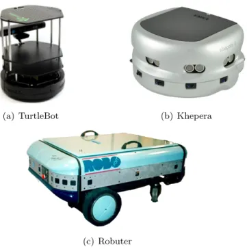
The differential drive kinematics consists in two active wheels, rotating on a common axis, driven by two different motors. In addition, one or more passive castor wheel(s) can support the robot stability without interfering with the robot kinematic. Many commercial robots adopt this kind of mech-anism due to the simplicity of implementation, the relative low cost and the compactness of the system. We can find it in TurtleBot [13], Khepera [14] or Robuter [15], represented respectively in Figure 3.3(a), Figure 3.3(b) and Figure 3.3(c)
The whole robot motion is based on the difference in rotation velocity of the two active wheels. The ICC lies, as expected, on the wheels rotation
(a) TurtleBot (b) Khepera
(c) Robuter
Figure 3.3: Commercial differential drive robots
axis and the curve that the robot will follow depends on the position of this point with the respect of the middle point between the two wheels, as shown in Figure 3.4. The relationship between the wheels velocity vr and vl, the distance between the ICC and the midpoint of the wheels R, and the angular velocity of the robot ω are given by the following
ω(R + l
2) = vr, ω(R − l
2) = vl,
(3.6)
where l is the distance between the 2 wheels.
We are actually interested in retrieving R and ω00 from the velocities, which are usually the available data given by the encoders, and l which is a fixed parameter. So the formulas are:
R = l(vr+ vl) 2(vr− vl),
ω = vr− vl
l .
(3.7)
It is interesting to analyze a couple of special cases. When vr = vl then R = ∞, which means that the robot is moving in a straight line. When
Figure 3.4: Differential drive kinematics
vl = −vr then R = 0, which means that the robot is only rotating around the vertical axis passing through the midpoint between the wheels.
Since the differential drive structure is non-holonomic, the robot is not able, for example, to perform a lateral movement or any other kind of dis-placement not represented by the previous equations. The position (x0, y0, θ0) at a particular instant of time is given by the computation on the previous (x, y, θ) and the time span ∆t between the two positions
x0 y0 θ0 = cos(ω∆t) −sin(ω∆t) 0 sin(ω∆t) cos(ω∆t) 0 0 0 1 x − ICCx y − ICCy θ + ICCx ICCy ω∆t , (3.8)
where ICCx and ICCy are the coordinates computed as it follows: ICC = (x − Rsin(θ), y + Rcos(θ))
The specific case for the odometry calculation in differential drive, according with 3.2 is x(t1) = 1 2 Z t 0 (vr(t) + vl(t))cos(θ(t))dt y(t1) = 1 2 Z t 0 (vr(t) + vl(t))sin(θ(t))dt θ(t) = 1 l Z t 0 (vr(t) − vl(t))dt (3.9) 33
Figure 3.5: Differential drive robot motion from pose (x, y, θ) to (x0, y0, θ0)
3.2.3 Skid-steering odometry
The skid-steering mechanics tries to maintain the simplicity and compact-ness of the differential drive model, improving in the meantime its robust-ness. It consists in four wheels that we can consider separately as a pair on the left, front and rear, and a pair on the right, again front and rear. Each couple of wheels is driven by one motor, located in the middle of the front and rear wheel. These two wheels are usually connected by a transmission belt or a chain. Each motor allows to rotate the pair of wheels connected at with the same velocity.
Skid-steering compactness and the high maneuverability [16][17], in ad-dition to the higher robustness, with the respect of the differential drive, make this kind of mechanic an optimal choice for different purposes [18][19]. This mechanics, indeed, offers a good mobility on different terrains, not only indoor, but also outdoor ones, because one of its advantages is the possibil-ity of installing tracks for the terrains that require them, without changing the whole mechanic.
Unfortunately, the drawback is a more complex kinematics because the pure rolling and no-slip assumption - which was possible to use for the differ-ential drive case - is no more an option: the wheels must slip during a curve. This implies a hard-to-predict motion, given the velocity input. Other dis-advantages are an energy inefficient motion and a fast tires’ consumption, caused by the slippage needed for curving [20].
Wang et al. [21] help to partially resolve the problem of the complex skid-steering kinematic proposing an approximation to the differential drive
Figure 3.6: Ra.Ro. wheels
kinematic based on three assumptions:
(i) the mass center of the robot is located at the geometric center of the body frame
(ii) the two wheels of each side rotate at the same speed (wf r = wrr and wf l = wrl)
(iii) the robot is moving on a firm ground surface, and all the four wheels are always in contact with the ground surface
Then, considering the Figure 3.7 and the deriving the Equations 3.9 we obtain vx vy wz = f " wlr wrr # (3.10)
where v = (vx, vy) represents the vehicle’s translational velocity with respect to its local frame, wz represents its angular velocity, r represents the radius of the wheels and wl and wr represent respectively the angular velocity of the left and right wheels.
While the robot is curving there are different ICR: ICRl, ICRr and ICRG, that belongs respectively of the left-side tread, right-side tread, and the robot center of mass, as shown in Figure 3.5. We define the coordinates of the ICRs respect to the local frame as (xl, yl), (xr, yr) and (xG, yG). All of the treads share the same angular velocity ωz, so these equations follows
yG= vx
wz , (3.11)
Figure 3.7: Skid-steering platform yl = vx− wlr wz , (3.12) yr = vx− wrr wz , (3.13) xG = xl= xr= − vy wz . (3.14)
From (3.9) to (3.14) the generic odometry kinematic (3.2) can be repre-sented as: vx vy wz = Jw " wlr wrr # . (3.15)
where Jw depends on IRCs coordinates and is defined as follows:
Jw = 1 yl− yr −yr yl xG −xG −1 1 . (3.16)
When the robot is symmetrical, then the ICRs lies symmetrically on the x-axis, and we have xG = 0 and y0 = yl= −yr. The Jw matrix can be rewritten as:
Figure 3.8: Geometric equivalence between the wheeled skid-steering robot and the ideal differential drive robot
Jw = 1 2y0 y0 y0 0 0 −1 1 . (3.17)
So the velocities defined in Equations 3.15 can be defined, for the sym-metrical model, as follows:
vx= vl+ vr 2 vy = 0 wz= −vl+ vr 2y0 (3.18)
and from Equation 3.7 we can get the instantaneous radius of the path curvature: R = vG wz = vl+ vr −vl+ vr y0. (3.19)
The ratio between the sum and difference of left and right wheels linear velocities [22] can be defined as a variable λ:
λ = vl+ vr
−vl+ vr , (3.20)
and Equation 3.19 becomes:
R = λy0. (3.21)
A similar approach is used in Mandow’s work [23], in which an IRC coefficient χ is defined as:
χ = yl− yr
B =
2y0
B , χ ≥ 1 (3.22)
χ represents the approximation from the differential drive kinematic. We can notice that when χ is equal to 1 there is no slippage and the skid-steering model coincides with the differential drive. It implies that we can approximate the skid-steering model as a differential drive model, working on the χ variable. In particular, the skid-steering coincides with a differential drive with a larger span between the left and right wheels as shown in Figure 3.8. This is a very useful method and it will be very useful for our work.
3.3
Sensor fusion framework
As mentioned before, pure kinematics equations are actually just an ap-proximation of the real world, they are not sufficient to retrieve the correct odometry of a robot with enough precision. This is why multi-sensor fusion is required. Here we introduce the framework used to make this process in a way possible to set up.
3.3.1 ROAMFREE
The acronym ROAMFREE stands for Robust Odometry Applying Multi-sensor Fusion to Reduce Estimation Errors. The main aim of the frame-work is to offer a set of mathematical techniques and to perform sensor fusion in mobile robotics, focusing on pose tracking and parameter self-calibration [24]. The main goals of the ROAMFREE project include ensur-ing that the resultensur-ing software framework can be employed on very different robotic platforms and hardware sensor configurations and easily tuning to specific user needs by replacing or extending its main components.
In ROAMFREE the information fusion problem is formulated as a fixed-lag smoother whose goal is to track not only the most recent pose, but all the positions and attitudes of the mobile robot in a fixed time window: short lags allow real time pose tracking, still enhancing robustness with respect to measurement outliers; longer lags allow for online calibration, where the goal is to refine the available sensor parameters estimation.
The system is based on a graph-based approach. In particular, a factor graph is generated; this graph keeps the probabilistic representation of the
pose retrieved by the sensor fusion measurements, the estimated sensor pa-rameters and the sensor error models. All the modules interact in some way with this graph, for example to update it with new measurements or new estimated poses. The factor graph is designed to allow an arbitrary number of sensors, even if they work at different rates, without a predictable rate or producing obsolete data.
The framework implements a set of logical sensors, which are indepen-dent from the actual hardware that produces the measurement. For ex-ample, an odometry measurement can be retrieved from a laser scanner elaboration or a wheels’ encoders one, but both can be properly setted up as a logical GenericOdometer sensor. Each logical sensor is characterized by a parametric error model specific to its domain. This means that we must initialize the sensors passing the specific parameters for that sensor. For example, a DifferentialDriveOdometer requires the wheels radii and the wheels distance, expressed in meters. Another required parameter to prop-erly set up a sensor is its position and orientation with the respect to the tracked base frame. For example, the camera sensor, possibly used to re-trieve markers positions, must be properly set in order to calculate the exact transformation between the marker seen and the base frame.
ROAMFREE’s modularity and its ROS implementation make it a very powerful tool for sensor fusion purposes. Unfortunately we had to deal with a lack of documentation which made the development of a stable ROS node quite hard.
Factor graph filter As mentioned before, the core of ROAMFREE lies in the factor graph filter. We have already written about the important fea-tures of graph-based approaches in Subsection 3.1.2 in a general way. The most relevant advantage is the possibility of manage high-dimensional prob-lems in a relatively short time. The graph holds the full joint probability of sensor readings given the current estimate of state variables, representing its factorization in terms of single measurement likelihoods. Each node of the graph contains a the pose of the robot and the sensors’ calibration pa-rameters, i.e. gains, biases, displacement or misalignments. The nodes are generated by new measurements, represented as hyper-edges (factors) con-necting one or more nodes, depending on their order. For example, a velocity measurement connects two nodes since it needs one integration to retrieve a position; an acceleration needs three nodes because two integrations are required.
We need to choose one, and only one, of the available sensors as an architecture master sensor, and a good practice is to choose an odometry
Figure 3.9: An instance of the pose tracking factor graph with four pose vertices ΓW O(t)
(circles), odometry edges eODO(triangles), two shared calibration parameters vertices
kθand kv(squares), two GPS edges eGP S and the GPS displacement parameter S (O) GP S
sensor to play this role, because it usually has a high rate and it is the one that gives a hopefully good starting point for the optimization process. Once the master sensor measurement is collected, an initial guess of the new pose is made and then a non-linear optimization process begins, also using the other measurements retrieved in the meantime. It can happen that sensor readings are late for low rate, connection problems or in general are not available. In these cases, if the available ones are not sufficient to generate a pose, the measurement handling is delayed until enough data are available. Node generation is based on a fixed-lag window. It means that only the nodes contained in this time span are considered for the following pose. Older nodes and factors, since are no more used, are deleted. In order to avoid high loss of information older nodes and factors can be marginalized, keeping the information they used to hold in a new generated factor.
We can resume the factor-graph advantages here:
• Flexible with respect to sensor nature and number. The modularity of the system allows to manage all the inserted sensors in an independent and uniform way, by means of the abstract hyper-edges interface, as they are inserted into the graph.
• Sensors can be, if necessary, turned on and off during the process. The factors management is asynchronous, so they can be added into the graph as soon as new readings are available.
infor-mation is received, according to its time stamp, it is not discarded, but an appropriate factor is created, connecting the nodes interested by it and consequentially updating and refining them.
• The resulting estimation is higher in quality and, in certain circum-stances, i.e., with many state variables faster than traditional filters, such as EKFs [8].
• The high degree of sparsity of the considered information fusion prob-lem is explicitly represented and it can be exploited by inference al-gorithms. Indeed, in our case a factor may involve up to three robot poses; moreover, it is difficult to imagine a robot employing much more than ten sensors for pose estimation, implying that each pose is incident to a limited number of factors.
Error models For each logical sensor model an error model definition is needed. All of theme come a common definition
ei(t) = ˆz(t; ˆxSi(t), ξ) − z + η , (3.23) where ˆxSi(t) represents the extended state for the sensor frame Si in which the position and the orientation of the frame with the respect of the world frame at time t; ξ represents the vector of the parameters relative to that sensor and ˆz(t; ˆxSi(t), ξ)) is a predictor measurement computed as a function of the previously defined parameters and the incident nodes. z is the real sensor output and η is a zero-mean Gaussian noise representing the mea-surement uncertainty. It is evident that the more the prediction is accurate, the more the error is near to 0, net of the Gaussian noise.
The equation that describes the actual error depends on the type of measurement considered. We can identify five classes:
(i) absolute position and/or orientation (e.g., GPS)
(ii) linear and/or angular velocity in sensor frame (e.g., gyroscope) (iii) acceleration in sensor frame (e.g., accelerometer)
(iv) vector field in sensor frame (e.g., magnetometer) (v) landmark pose with respect to sensor (e.g., markers)
Moreover, the other thing that characterize the sensor in ROAMFREE is the parameter’s vector ξ, which includes gain, bias and other specific parameters according to the sensor class. These parameters sometimes are
Figure 3.10: ROAMFREE estimation schema
easy to retrieve from sensors specifications or from observation, but they often need an accurate tuning to let everything work properly.
Every time a measurement is added to the factor-graph we need to pass as parameter also the covariance matrix ,in addition to the measurement itself and the sensor name.. Usually, in ROAMFREE, is used a diagonal matrix, with the measurement variances on the diagonal, and zeros other-wise. We must be careful in covariance matrix setup. Changing the value of the variances means to change the reliability of a sensor. In other words, if two measurements indicate two conflicting outputs, the system will trust more the one with a lower covariance. The covariance matrix can be even different according to the actual measurement, of course always being of the right dimension.
A convenient feature is the outlier management made through the robust kernel technique. It consists in setting a threshold in the measurement domain. If this threshold is exceeded in module, the error model of the sensor, for that measurement, becomes linear instead of quadratic, which means that it is less involved in the subsequent computation. This is useful to deal with errors that can sometimes occur in data retrieving.
Optimizations The optimization algorithms implemented in ROAMFREE are Gauss-Newton and Levenberg-Marquardt. Both of them require a prob-lem formulated as a non-linear, wighted and least-squares optimization and here we will discuss about how this is done. Considering the error function ei(xi, η) associated to the i-th edge of the hyper-graph and defined as (3.23). We can approximate the error function as ei(xi) = ei(xi, η)|η=0 since ei is a random vector. It can involve non-linear dependencies with respect to the noise, so its covariance Ση is computed by means of linearization, i.e.:
Σei = Ji,ηΣηJ T
i,η|xi=˘xi,η=0 (3.24) where Ji,η is the Jacobian of ei with respect to η evaluated in η = 0 and in the current estimate ˘xi. The covariance matrix Ση is the one we mentioned before and here is where it is involved in the optimization.
A negative log-likelihood function can be associated to each edge in the graph, which stems from the assumption that zero-mean Gaussian, noise corrupts the sensor readings. Omitting the terms which do not depend on xi, for the i-th edge this function reads as:
Li(xi) = ei(xi)Ωeiei(xi) (3.25) where Ωei = Σ
−1
ei is the information matrix of the i-th edge. The solution to the information fusion problem is given by the assignment for the state variables such that the likelihood of the observations is maximum.
P = argmin x N X i=1 Li(xi) (3.26)
We can observe that this is a non-linear least-squares problem where the weights are the information matrices associated to each factor. If a reason-able initial guess for x is known, a numerical solution for P can be found by means of the popular Gauss-Newton (GN) or Levenberg-Marquardt (LM) algorithms. A complete schema of the interaction among the ROAMFREE modules is represented in Figure 3.10.
3.4
Simultaneous Localization and Mapping
With simultaneous localization and mapping (SLAM) is meant the building of a map while the robot locates itself into the map that is being created. The SLAM can be considered as a preliminary phase in which the robot creates the map which it will use for the autonomous navigation, or it can be contextual to the autonomous navigation. It is important to point out that it does not matter whether the robot, during the SLAM phase, is human-controlled or not.
Although the first localization guess is given by the odometry, as men-tioned in Section 3.2, it accumulates error as long as the robot moves. A good odometry estimation is desirable for the SLAM problem, but the error given by the odometry can be corrected by using world references observed through laser scanner(s), camera(s) (Visual SLAM) or similar sensors. It follows that the observation should be done in an environment as static as
possible, even if SLAM frameworks can deal with mobile objects. Moreover, the localization makes sense if it is made with respect of a map, but if the map is being made at the same time is evident the possible problem that can occur. SLAM must be done in a recursive way and this is one of the main reasons why it is such a complex task.
From a probabilistic point of view, there are two main forms of SLAM. One is known as the online SLAM problem algorithm which involves esti-mating the posterior over the momentary pose along with the map:
p(xt, m|z1:t, u1:t) , (3.27)
Here xtis the pose at time t, m is the map and z1:t and u1:t are the measure-ments and controls, respectively. This problem only involves the estimation of the variables that exist at time t. Algorithms for the online SLAM prob-lem are incremental: they discard past measurements and controls once they are processed. The second SLAM problem is called the full SLAM problem. Here we want to calculate a posterior over the entire path x1:t along with the map, instead of just the current pose xt:
p(x1:t, m|z1:t, u1:t) (3.28)
Instead of incrementally computing the state as in the online case, here the sequence of states is computed once.
Regardless of the method used to implement a full or online SLAM, the algorithm must follow these steps:
(i) Landmarks detection: the robot must recognize some features from the environment, called landmarks. Considering a 2D map, horizontal LIDAR are the most common sensor used for this kind of task. An-gles, edges, particular shapes are good candidates to be detected as a landmark.
(ii) Data association: once the landmark is been detected, it must be matched with a possibly existing landmark into the map. It can be a hard task because a single feature can match with many, growing exponentially as long as the map grows.
(iii) State estimation. It uses observations and odometry to reduce errors. The convergence, accuracy, and consistency of the state estimation are the most important properties. Thus, the SLAM method must main-tain the robot path and use the landmarks to extract metric constraints to compensate the odometer error.
Figure 3.11: The image represents the topics subscribed and published by the mapping node, independently of the exact mapping system used
The major difficulties of SLAM are the following:
• High dimensionality: since the map dimension constantly grows when the robot explores the environment, the memory requirements and time processing of the state estimation increase. Some submap-ping techniques can be used to reduce these consumption, at the cost of a worse performance.
• Loop closure: when the robot returns to a place it has been previ-ously, the accumulated odometry error might be large. Then, the data association and landmark detection must be effective in correcting the odometry. Place recognition techniques are used to cope with the loop closure problem.
• Dynamics in environment: state estimation and data association can be confused by the inconsistent measurements in the dynamic environment. There are some methods that try to deal with these environments.
We will focus on 2D SLAM, using a laser scanner as a sensor and related laser scans measurements. In general, the aim of a SLAM framework is to collect the laser scans and try to associate them in one occupancy grid map. Then, if following scans match with the memorized map, the position will be corrected according to this match, hopefully improving the localization estimation. The more various the environment is, the more the localization is easy to make, because the probability to deal with a potential ambiguity is lower.
Algorithm 2 Improved RBPF for map learning Require:
St−1, the sample set of the previous time step
zt, the most recent laser scan
ut−1, the most recent odometry measurement
Ensure:
St, the new sample set
St= { }
for all s(i)t−1∈ St−1do
hx(i) t−1, w (i) t−1, m (i) t−1i = s (i) t−1 //Scan − matching x0 (i)t = x(i)t−1⊕ ut−1 ˆ
x(i)t = argmaxxp(x|m(i)t−1, zt, x0 (i)t )
if ˆx(i)t = failure then x(i)t ∼ p(xt|x(i)t−1, ut−1)
w(i)t = w(i)t−1· p(zt|m(i)t−1, zt, x0 (i)t )
else
//Sample around the mode for all k = 1 to K do
xk∼ {xj| |xj− ˆx(i)| < ∆}
end for
//Compute Gaussian proposal µ(i)t = (0, 0, 0)T
η(i)= 0
for all xj∈ {x1, . . . , xK} do
µ(i)t = µ(i)t + xj· p(zt|m(i)t−1, xj) · p(xt|x(i)t−1, ut−1) η(i)= η(i)+ p(z
t|m(i)t−1) · p(xt|x(i)t−1, ut−1)
end for µ(i)t = µ(i)t /η(i)
Σ(i)t = 0
for all xj∈ {x1, . . . , xK} do
Σ(i)t = Σ(i)t + (xj− µ(i)t )(xj− µt(i))T· p(zt|m(i)t−1· p(xt|x(i)t−1, ut−1)
end for Σ(i)t = Σ(i)t /η(i) //Sample new pose x(i)t ∼ N (µ(i)t , Σ
(i) t )
//U pdate importance weights w(i)t = w(i)t−1· η(i)
end if // U pdate map
m(i)t = integrateScan(m(i)t−1, x(i)t , zt) // U pdate sample set
St= St∪ {hx(i)t , w (i) t , m (i) t i} end for Nef f= 1 ΣN i=1( ˜w(i))2 if Nef f< T then St= resample(St) end if 3.4.1 Gmapping
gmapping is the most widely used laser-based SLAM package in robotic field, worldwide. The algorithm was proposed by Grisetti et al. in 2007 and it is a Rao-Blackwellized Particle Filter SLAM approach [25].
We mentioned the Particle Filter in Subsection 3.1.1 and here we will describe RBPF, which is an optimized version for the SLAM problems. Let’s start from (3.28) and factorize it as:
this factorization allows to first estimate only the trajectory of the robot and then to compute the map given that trajectory. In particular, p(m|x1:t, z1:t) can be easily computed using “mapping with known poses” since x1:t and z1:t are known.
If new control data ut from the odometry and a new measurement zt form the laser scanner is available; the RBPF occupancy grid SLAM works as follows.
1. It determines the initial guess x0t(i), based on ut and the pose, since the last filter t update xt−1 has been estimated.
2. It performs a scan matching algorithm based on the map m(i)t−1 and x 0(i) t . If the scan matching fails, the pose x(i)t of particle i will be determined according to a motion model, otherwise the next two steps will be per-formed.
3. If the scan matching is successfully done, a set of sampling points around the estimated pose ˆx(i)t of the scan matching will be selected. Based on this set of t poses, the proposal distribution will be estimated.
4. It draws pose x(i)t of particle i from the approximated Gaussian distribu-tion of the improved proposal distribudistribu-tion.
5. It performs an update of the importance weights.
6. It updates map m(i) of particle i according to x(i) and zi.
The more detailed RBPF algorithm pseudo-code can be read in Algo-rithm 2. The author proposes a way to compute an accurate distribution by taking into account both the movement of the robot and the most re-cent observations. This decreases the uncertainty about the robot’s pose in the prediction step of the particle filter. As a consequence, the number of particles required decreases since the uncertainty is lower, due to the scan matching process, improving the performance.
3.4.2 Cartographer
Another possible approach to the SLAM problem is using graph-based meth-ods. These methods use optimization techniques similar to the factor graph previously introduced to transform the SLAM problem into a quadratic pro-gramming problem. The historical development of this paradigm has been focused on pose-only approaches using the landmark positions to obtain con-straints for the robot path. The objective function to optimize is obtained
assuming Gaussianity. Since these methods are based on a factor graph, they are able to better remember the previous sub-maps and the previous localization and thus they prove to be more accurate with respect to other approaches. On the other hand, their main disadvantage is the high compu-tational time they take to solve the problem, for this reason they are usually suitable to build maps off-line.
Google’s Cartographer provides a real-time solution to indoor and out-door mapping. The system generates submaps from the matching of the most recent scans at the best estimation position, which is assumed to be ac-curate enough for short periods of time. Since the scan matching only works on submaps, the error of the pose estimation in the world frame eventually increases. For this reason, the system runs periodically a pose optimization algorithm. When a submap is considered to be finished, no more scans are added to it and it takes part in scan matching for loop closure. If the robot estimated pose is close enough to one or more processed submaps, the algo-rithm runs the scan matching between the incoming laser scans and those maps. If a good match is found, it is added as a loop closing constraint to the optimization problem. By completing the optimization every few sec-onds, the loops are closed immediately once a location is revisited. This leads to the soft real-time constraint that the loop closure scan-matching has to happen before the new scans are added, otherwise it will fall behind noticeably. This has been achieved by using a branch-and-bound approach and several precomputed grids per finished submap.
3.5
Localization
As mentioned before, robot localization is the problem of estimating a robot pose relative to the map of the operational environment. It has been defined as one of the most fundamental problems in mobile robotics [26].
We can recognize different levels of localization problems. The localiza-tion tracking is the simplest one; the robot starts from a known posilocaliza-tion and the localization aim is to correct the hopefully small odometry errors. A more challenging problem is the global localization problem; the robot must localize itself without a given initial position. An even more difficult problem is the kidnapped robot problem [27]; it can happen when a localized robot is moved, with no information about this transportation, to a different location. It might seem a similar problem to the second one, but here we can not trust a measurement as consistent with a previous one, because of the loss of information during the unexpected movement.
Algorithm 3 Adaptive variant of Monte Carlo Localization
1: procedure AMCL(Xt−1, ut, zt, m)
2: Xt= Xt= 0
3: for all m := 1 toM do
4: x(m)t = SampleMotionModelOdometry(ut, x(m)t−1) 5: w(m)t = MeasurementModel(zt, x(m)t , m); 6: Xt= Xt− hx(m)t , w (m) t i 7: wavg = wavg+ 1 Mw (m) t 8: end for
9: wslow = wslow+ αslow(wavg− wslow)
10: wf ast= wf ast+ αf ast(wavg − wf ast)
11: for all m := 1 to M do
12: with probability max(0.0,1.0 - wf ast wslow) do
13: add random pose to Xt
14: else
15: draw i ∈ {1, . . . , N } with probability ∝ x(m)t
16: add x(i)t to Xt
17: end with
18: end for
19: return Xt
20: end procedure
In other words, the localization problem consists in identifying an appro-priate coordinate transformation between the global frame, which is fixed and integral with the map, and the robot frame. Then, a detected object from the robot’s point of view can be, in turn, transformed with the respect of the global frame by coordinate transformation.
In robot localization the state xtof the system is the robot pose, which for the two dimensional mapping, is typically represented as a three dimensional vector xt = (x, y, θ) in which x and y indicate the position of the robot in the map plane, and θ the angle formed by the robot orientation. The state transition probability p(xt|xt−1, ut−1) describes how the robot position changes given the previous position xt−1and the new sensors’ measurements ut−1. The perceptual model p(zt|xt) describes the likelihood of making the observation ztgiven that the robot is at position xt.
3.5.1 Adaptive Monte Carlo Localization (AMCL)
The Adaptive Monte Carlo Localization (AMCL) is a method to localize a robot in a given map. It is an improved implementation of a particle filter. The word “adaptive” means that the number of particle used for the Monte Carlo localization is not fixed, but changes according to the situation. This number of particles is retrieved using the KLD-Sampling (Kulback-Leibler-Divergence) [28] [29]. The AMCL pseudocode algorithm is reported in Algorihm 3. It requires the set of particles of the last known state Xt−1 and the control data utfor the prediction; the measurement data ztand the map m for the update.
The algorithm returns the new state estimation as a set of particles Xt. This filter implementation is able to deal with the global localization problem, the localization tracking and the kidnapping problem. The AMCL is flexible with the respect of the resampling technique, that means that an arbitrary one can be used. Another advantage is that AMCL is able to recover from localization errors by adding some random particles to the Xt set, after a specified decade (lines 15 and 16 of 3). An AMCL ROS package is available [30] and a lot of robots use this package for the localization since it provides a good configuration parameter suite.
3.6
A note on ROS reference system
Developers of drivers, models, and libraries need a share convention for co-ordinate frames in order to better integrate and re-use software components. Shared conventions for coordinate frames provide a specification for devel-opers creating drivers and models for mobile bases. Similarly, develdevel-opers creating libraries and applications can more easily use their software with a variety of mobile bases that are compatible with this specification. In this chapter we will explain the reference frames that should be used for a localization system, according to the ROS standard [31].
Coordinate frames
base link The coordinate frame called base link is rigidly attached to the mobile robot base. The base link can be attached to the base in any arbitrary position or orientation; for every hardware platform there will be a different place on the base that provides an obvious reference point. A right-handed chirality with x forward, y left and z up is preferred.