Agent-based modelling analysis of the market penetration of fuel cell vehicles in Germany

(1)

Politecnico di Milano

School of Industrial and Information Engineering

Energy Department

Forschungszentrum Jülich

Institute of Energy and Climate Research

Electrochemical Process Engineering (IEK-3)

Agent-Based Modelling Analysis of

the Market Penetration of Fuel Cell

Vehicles in Germany

Master thesis

by

Simone Delli Compagni

Matriculation number: 817046

Supervisor at Forschungszentrum Jülich: Schiebahn Sebastian, Dr.

Supervisor at Politecnico di Milano: Silva Paolo, Prof.

(2)

(3)

Abstract

Concerns about climate change and the problem of supply security of fossil fuels brought the German government to set the ambitious goal of covering 80% of the gross electricity consumption with renewables energies within 2050. Due to the fluctuating nature of these energy sources and grid limitations, large amounts of excess energy are likely to be available on the grid if this target is to be met. A promising use for this surplus energy is producing hydrogen to power fuel cell vehicles. Yet the successful introduction of this new technology is likely to present a barrier: car manufacturers will not produce fuel cell vehicles until filling stations start selling hydrogen, whereas the refuelling infrastructure will not develop unless a significant number of fuel cell vehicles on the road is observed. In order to overcome this obstacle, referred to as “chicken and egg problem”, policy is needed. In this master thesis, an agent-based model is implemented to investigate the effect that a tax on internal combustion engine vehicles or a subsidy for fuel cell vehicles, coupled with different refuelling infrastructure development programs, would have on the market penetration of fuel cell vehicles. Analysing this model will help gain deeper insights about how to design a policy to foster the diffusion of this new technology, making sure to minimise negative effects on consumers and on the automotive industry.

Key Words: Agent-based modelling, Fuel cell vehicles, Hydrogen economy, Hydrogen

infrastructure, Market penetration

Sommario

La preoccupazione per il cambiamento climatico e il problema della sicurezza dell’approvvigionamento energetico hanno portato il governo tedesco a stabilire l’ambizioso obiettivo di coprire l’80% del consumo elettrico con le energie rinnovabili entro il 2050. A causa dei vincoli della rete elettrica e della variabilità di queste fonti, grandi quantità di energia in eccesso sarebbero presenti sulla rete se questi obiettivi fossero raggiunti. Una promettente soluzione per l’utilizzo di questa energia è la produzione d’idrogeno da usare come combustibile in veicoli fuel cell. La diffusione dei veicoli a idrogeno presenta tuttavia un ostacolo: le case automobilistiche non cominceranno a produrre veicoli fuel cell fino a quando un determinato numero di stazioni di rifornimento non comincerà a vendere idrogeno, mentre l’infrastruttura per l’idrogeno non si svilupperà finché non sarà possibile osservare un numero significativo di veicoli fuel cell sulle strade. Questo ostacolo, cosiddetto dilemma “uovo-gallina”, può essere superato con l’aiuto di politiche incentivanti. In questa tesi un modello basato su agenti è stato implementato al fine di analizzare l’effetto che una tassa sui veicoli con motore a combustione interna o un sussidio per i veicoli fuel cell, abbinati con un piano di sviluppo dell’infrastruttura per il rifornimento d’idrogeno, avrebbe sulla diffusione dei veicoli fuel cell. Analizzare questo modello aiuterà ad acquisire le conoscenze necessarie a sviluppare un’efficace politica incentivante, limitando gli effetti negativi sui consumatori e sull’industria dell’auto.

(4)

(5)

Declaration of originality

Hiermit versichere ich, die vorliegende Arbeit selbständig und ohne Hilfe Dritter angefertigt zu haben. Gedanken und Zitate, die ich aus fremden Quellen direkt oder indirekt übernommen habe, sind als solche unter Angabe der Quelle als Entlehnung kenntlich gemacht. Dasselbe gilt sinngemäß für Tabellen, Karten und Abbildungen. Diese Arbeit hat in gleicher oder ähnlicher Form noch keiner Prüfungsbehörde vorgelegen und wurde bisher nicht veröffentlicht.

_________, den ___________ _______________________

(6)

(7)

Table of contents

1 Introduction

1.1 Motivation

Increase in climate change awareness and limited security of supply of fossil fuels are pushing towards a future in which most of the electric power is bound to be produced from renewable energy sources (RES). This is especially true for Germany, where, due to the ambitious goals set by the government with the Renewable Energy Act (Erneuerbare-Energien-Gesetz), 40% to 45% of the gross domestic power consumption is set to be covered by renewable energy sources by 2025, with this number increasing to 55% to 60% in 2035 and 80% in 2050 (EEG, 2014). If the renewable installed power increases to meet these targets and the number of conventional power plants decreases, large quantities of excess power will be available on the grid due to fluctuations of RES and grid limitations. Fig. 1 shows an estimate of the surplus power distribution in Germany at the county level. These results are based on the assumptions that the installed renewable power will follow (EEG, 2014) and that all the projects for the extension of the grid indicated in the German grid development plan will be realised within 2035. As the figure shows, considerable amounts of surplus energy will be observed as soon as 2025, most of which in the north of Germany, where most of the large offshore windfarms are located. Under each graph, an estimation of the total value of excess power in the whole country is indicated: this value is extremely high for the year 2050, considering that the total electric power consumption in Germany in 2015 was 576.5 TWh (IEA, 2015).

2025 2035 2050

(12)

1 Introduction

10

Reaching the above-mentioned targets requires the use of large-scale energy storage, which would allow to balance fluctuations in renewable energy production and store surplus power. The current storage capacity available in Germany, mainly represented by pumped storage hydropower, adds up to only 77 GWh (Kühne, 2012), which is orders of magnitude smaller than the estimates shown above. Storage capacity on the TWh scale can however be achieved storing surplus power in the form of chemical energy and a very promising option in this area is a process called “power to gas”. In this process, power from the grid is fed in large-scale electrolysers that convert it into hydrogen. The hydrogen produced in such a way can have different utilization paths, like producing methane or directly feeding it into the natural gas grid, but the best option from an economical standpoint is to use it in the transportation sector to power fuel cell vehicles (Schiebahn et al., 2015). In this solution hydrogen would become a link between two game-changing technologies, renewable energies and electromobility, coupling the two sectors with the highest total emissions in the country. With respectively 38% and 17% of the total CO2

emissions in Germany, the electricity and transportation sectors present in fact the highest potential for emissions reduction (Umweltbundesamt, 2014).

Fuel cells generate electricity via an electrochemical reaction in which oxygen and hydrogen are combined to form water. In fuel cell vehicles (FCVs), a fuel cell is used to generate electricity that powers an on-board electric motor: hydrogen from the tank and oxygen from the air are used as an input for the fuel cell. The absence of a combustion process and the use of an electric motor allow FCVs to reach overall efficiencies that are approximately twice as high as those of internal combustion engine vehicles (JRC, 2014). In addition, the use of fuel cell vehicles instead of internal combustion engine ones would allow for lower CO2 emissions, lower emission of local pollutants and reduced noise level

in cities.

Although very promising, such a solution presents several challenges: surplus power is not yet as high as to justify large-scale hydrogen production, large electrolysers like those needed for such a solution do not exist yet, there are only 22 hydrogen filling stations in Germany (CEP, 2016) and the total amount of registered FCVs in Germany is, simply put, negligible. Due to the lack of experience with such a new fuel and the high investments required to make this solution a reality, both car manufacturers and filling station owners are hesitant to enter this newly-born market. Without a refuelling infrastructure in place to support them, the auto industry is reluctant to start producing FCVs. Simultaneously, filling station owners will have no incentive to start selling hydrogen unless there is a significant number of FCVs on the road. The situation that FCVs face is known as chicken and egg problem, and poses the question “What comes first, the vehicle or the fuel?”

A solution to this dilemma can however be found in the use of policy, combined with an infrastructure development program: a tax on conventional vehicles or a subsidy for fuel cell vehicles, coupled with incentives to filling stations that start selling hydrogen, can help the FCVs market move past this barrier. In designing such a policy, it is nonetheless crucial to limit potential negative effects on the car market, especially in the light of its importance for the German economy.

(13)

1 Introduction In order to address this problem, an agent-based model is used in this master thesis to analyse the complex system made up of car manufacturers, consumers and filling station owners. This modelling technique follows a bottom-up approach that consists in defining the behaviour of single actors (called agents), like producers and consumers, and then observe the behaviour of the system as a whole when a policy to foster FCVs diffusion is applied. The model will allow gathering insights on the effects that a policy might have on the interested parties, so as to anticipate how they could be affected, where the oppositions might come from and where negative effects can be limited.

1.2 Aim of the thesis

The aim of this master thesis is developing an agent-based model based on (M. Schwoon, 2006) to study the diffusion of fuel cell vehicles in the German car market while demonstrating how such a model is implemented and analysed. The specific objectives are:

 Developing an agent-based model that will serve as a basis for future work;

 Showing how such a model is implemented and analysed and what kind of insights can be gathered from it;

 Comparing a tax on internal combustion engine vehicles and a subsidy on fuel cell vehicles as policy options to foster the diffusion of fuel cell vehicles in Germany  Comparing the obtained results with those provided by the model on which the

present one is based.

1.3 Structure

This master thesis is organised as follows:

Chapter 2 In this chapter, the theoretical foundations needed to understand agent-based modelling (ABM) are laid. After describing the characteristics of the systems that can be analysed with this modelling approach, the anatomy of such a model is described. At the end of the chapter, advantages and limitations of agent-based modelling are explained.

Chapter 3 This chapter describes the model in detail. In the first section, a general overview about the organization of the model is presented. In the rest of the chapter the behaviour of the agents, the underlying assumptions and the structure of their interactions are presented.

Chapter 4 This chapter provides a description of how the conceptual model was converted into software and its correct operation verified. The first section is about the choice of the modelling environment and the structure of the software implementation. The second section describes the verification process in detail.

(14)

1 Introduction

12

Chapter 5 In this chapter, the analysed scenarios and the calibration of the model are presented. First, the assumptions behind the scenarios and their structure are presented. Then, the calibration of single agent behaviour is discussed. Chapter 6 In this chapter results of the model are presented and discussed. In the first two sections, the results for tax and subsidy scenarios are described. In the third section, a brief evaluation of the environmental benefits of the market penetration of fuel cell vehicles is provided. In the fouth part, a sensitivity analysis of the crucial parameters is carried out. The fifth section deals with the differences in implementation and results between the original model and the present one. Finally, in the last section, the limitations of the model are discussed.

Chapter 7 The last chapter summarises the main points and conclusions of this master thesis. After presenting a short summary of its content, indications for future work on the model are provided.

(15)

2 Fundamentals of agent-based simulation

The following chapter aims at laying the necessary theoretical foundations needed to understand the complexities of agent-based simulation. First of all, complex adaptive systems, that agent-based modelling attempts to model, are defined and briefly described. After that, agent-based modelling (ABM) is compared to system dynamics as a modelling technique for complex adaptive systems. Lastly, the anatomy of an ABM is described in detail.

2.1 The concept of complex adaptive system

2.1.1 Definition of complex adaptive system

A complex adaptive system is a specific type of system often defined as a “complex macroscopic collection of relatively similar and partially connected micro structures formed in order to adapt to the changing environment and increase its survivability as a macro-structure” (MacLennan, 2007). Although this all-encompassing definition includes all the main features of complex adaptive system, a better understanding can be gained explaining the words that make up this name separately, starting with the definition of system.

A system consists of interacting and interrelated elements that act as a whole, where some pattern or order is to be discerned (Dam, Nikolic, & Lukszo, 2013). All systems (Ryan, 2008)

 are an idealization, meaning that they are an abstraction of a part of the real world;  have interdependent components that interact with each other forming patterns;  present emergent properties, that is to say properties that cannot be deduced just

looking at the single components, but result from the organization of these components;

 have boundaries;

 are enduring, since they have to last long enough to be observed;

 affect and are affected by the environment, which is simplified in modelling using a small number of relevant variables;

 exhibit feedback, since they contain loops in which A influences B and in turn B influences A;

 have non-trivial behaviour, that is to say they can react to a given input in a totally unexpected way.

A system is considered adaptive when it is capable of improvement over time in response to changes in the environment. In order for a system to be adaptive, it is not enough that

(16)

14

Finally a system is said to be complex when the whole can be considered more than the sum of its parts. Complexity implies that having a perfect knowledge about the behaviour of a group of single elements does not guarantee that it will be possible to predict what happens when those element are let interact in a system.

2.1.2 The concept of emergence

One of the most important properties of complex adaptive systems, that causes the complexity of their behaviour, is emergence. In system theory emergence is defined as a macro-level phenomenon that results from local-level interactions, and represents the overall system behaviour of a complex adaptive system. A very good example of emergence is given by a traffic jam, defined as a large number of vehicles on the road that are either unable to move or move very slowly. Although such a phenomena can be sometimes caused by an accident, it is, many other times, difficult to justify: the traffic jam emerges from the behaviour of single car drivers when certain conditions are met. The properties of the system that derive from this mechanisms are called emergent properties and are often counterintuitive: as an example, a traffic jam moves in the opposite direction to that of the cars that cause it. An interesting aspect of emergent properties is that they result from agent interaction and in turn constraint agent behaviour: the traffic jam is created by cars, and cars cannot move because of it. This causal relationship of a higher level to a lower level of the system is called downward causation and it is one of the effects of emergence.

2.1.3 Socio-technical systems

A socio-technical system is a complex system made up of two highly interconnected subsystems: a social network of actors and a physical network of technical artefacts (Allenby, 2006). A typical examples of socio-technical system is the electricity infrastructure. The technical subsystem is in this case made up of thousands of technical components, it provides electric power and includes power plants, the transmission and distribution grid, transformers and so on. The social subsystem is made up of all those actors that sell or buy electricity, like power plant owners, industrial consumers and private consumers, and by the legislative and regulatory framework that constraints the behaviour of these actors in the electricity infrastructure. Each actor in the social network makes decisions based on a certain set of rules, that can be studied more or less in depth depending on the focus of the system analysis. In this particular case the regulatory framework is very important, as can be deduced from what happened in the last 20 years in Europe: a change in rules from a vertically integrated system to a liberalised one brought about a lot of changes to which both consumers and producers had to adapt, completely reshaping the existing market. In this system the social network determines the development and operation of the technical system, which in turn affects the actors in the social network.

(17)

2.2 Modelling approaches

A model of a complex adaptive system is a formalisation of a modeller’s interpretation of reality and developing it the modeller is faced with two opposing needs. On the one hand the model should represent reality as accurately as possible, so that all the dynamics that one can observe in reality are also to be found in the model. On the other hand, the model should be simple enough to allow a better understanding of the modelled system: a model that is as detailed and as complex as what happens in the real world, would give the modeller no more information than studying reality directly.

Following the description given by (Dam et al., 2013) a model of a complex adaptive system should always possess three main characteristics: domain and multi-disciplinary knowledge, generative capacity and adaptivity. One of the defining characteristics of complex adaptive systems is that they cannot be thoroughly explained using a single formalism and this is why different points of view have to be considered in the study of these systems. As a consequence, developing a model for a complex adaptive system requires knowledge to be gathered from experts in different fields and also their active collaboration, since the modeller only has a partial understanding of the model complexity. Secondly, since a complex adaptive system is generated from the bottom up, the model will have to have a generative capacity. This means that the modeller will need to be able to “grow” the macroscopic regularity that can be observed in the real system using autonomous entities that interact with each other. Finally, the model has to be adaptive and be able to evolve over time: the individual entities‘ behaviour and the collective model behaviour should be able to mutate in response to selective pressures.

Due to the difficulties in developing a model that possesses all these characteristics, there is a tendency to solve these problems by reducing complexity and representing these systems using cost/benefit analysis, in which each system component is assigned a monetary equivalent. Yet there are modelling approaches that allow to address the problem on a more complex level. In modelling the market diffusion of innovations in general and the diffusion of alternative fuel vehicles in particular, the most used approaches that allow to retain complexity are system dynamics and agent-based modelling (Gnann & Plötz, 2015).

System dynamics is a modelling paradigm in which processes that happen in the real world are represented using delay structures and interacting feedback loops, that either balance or reinforce each other. From a mathematical point of view this representation corresponds to a system of differential equations and much of the modelling effort is spent on developing a structure that closely resembles the one observed in the real world. In system dynamics the main assumptions about a system’s behaviour lie in the global structure of the system and the effect of the global behaviour on the components is studied. In Agent-based modelling, on the other hand, the behaviour of the autonomous entities called agents and their interactions are simulated to study the effect that they have on the system as a whole. In ABM the structure of the model is not a precondition, as

(18)

16

The main difference between these two approaches is that agent-based modelling follows a bottom-up approach, in which the behaviour of the model emerges from the interaction of lower-level components of the system, while in system dynamics, that follows a top-down approach, the rules that describe the global behaviour must be chosen beforehand. In modelling complex adaptive systems the use of ABM can be advantageous when the modeller has no complete understanding about how the different parts of the model interact and cannot, as a consequence, set up a model description of unknown or partially-known behaviours.

ABM is particularly suited to model socio-technical systems. Assuming that the behaviour of real actors can actually be captured by the model, agent-based simulations allows the modeller to observe how the social part and the technical part of a complex system co-evolve and what is the system behaviour that can emerge due to this co-evolution. Running ABM simulations the modeller can conduct ex-ante analyses of the possible outcomes of a certain decision or solution to be better informed about what could happen if this solution is applied to the real system. It should be remembered though that ABM is no “crystal ball” that can predict the future: its goal is helping in the decision-making process, more often than not pointing at “what could go wrong” if a certain solution to a problem is deployed.

Further explanations about when to use ABM, its advantages and limitations are given in section 2.3.3.

2.3 Agent-based Modelling

Even though the concept of agent-based modelling (ABM) was first introduced in the late 40s, it can still be considered a relatively new approach to system modelling, since, due to its computational-intensive requirements, it only started being used in the 90s.

As anticipated above ABM is a modelling approach meant to examine the global effects caused by interactions of low-level entities in a complex adaptive system. These global effects emerge from the combined actions of all the agents, which are determined by a set of behaviour rules, and bring to results that can be surprising or difficult to predict otherwise. Agent-based modelling should not be confused with multi-agent system: even though these two modelling techniques can look similar, their goal is different. While in ABM agents are set up with the characteristics of real world equivalents and then emergent phenomena are observed, in multi-agent systems agents characteristics are set so that a certain emergence is obtained as a result.

ABM can be used to try and replicate complex phenomena that can be witnessed in reality and for which it is difficult to determine how things evolved in that specific way. Making assumptions about the behaviour of the single agents and causing the system to evolve similarly to reality can bring an understanding of how the system got there in the first place. Studying an agent-based model can be compared to being a new employee in a company: it takes a while to understand who relates to whom and how, because the pattern of relationships is not yet perceivable. After becoming familiar with the new environment, however, the pattern becomes clear. As it is usually said in the field of

(19)

2 Fundamentals of agent-based simulation generative science, “If you did not grow it, you did not explain it” (Epstein, 1999). Another promising possibility is using ABM to infer what it takes to make something happen, and this is exactly the type of question that this master thesis tries to answer for the successful difussion of fuel cell vehicles.

2.3.1 The agent

Following the definition given by (Jennings, 2000) an agent is an encapsulated computer system that is situated in some environment and that is capable of flexible, autonomous action in that environment in order to meet its design objectives. Agents

 are encapsulated, that is to say they have well-defined boundaries and interfaces;  are situated in a particular environment, meaning that they receive inputs about

the state of their environment through sensors and act on the environment through effectors;

 have design objectives, that means they have a specific goal to achieve;

 are autonomous, that is to say they have control over their internal state and their own behaviour;

 are capable of flexible problem solving behaviour, meaning that they can respond to changes in the environment and act in anticipation of future goals.

The agent is the smallest part of an agent-based model and its structure can be divided into states and rules.

A state is a collection of parameters that defines an agent at a given moment (Wooldridge & Jennings, 1995). States can be divided into internal state (only pertaining to one agent), local state (includes the internal state and the public variables of the agents that interact with the current one) and global states (all the relevant states in the observable environment). Imagining an application of ABM to the example of the electricity infrastructure, industrial consumers are agents whose internal states are represented by parameters like the amount of power they buy each year, the voltage level at which they take power from the grid and so on. The local state includes, besides the internal variables, also those of the neighbouring consumers that can be directly observed, like which electric company they buy electricity from. The state that contains all the variables accessible to one agent in the model is called global state. In this example the global state also contains variables like the price of electricity or the amount of taxes on electricity purchase.

Rules (or behaviours), on the other hand, define how an agent acts based on its internal, local or global state. This rules can have different characteristics and structures: the agent might act in some specific way if a parameter has a specific value and act in a completely different way if the parameter has another value (if-else statements). In some other cases the agent might choose how to act from a list of different possibilities based on the value of a utility function. An industrial consumer, for example, can decide to change the electric

(20)

18

All the agents in the ABM are contained in the environment: the environment contains all the information that the agents need to make decisions, that are not part of the internal state. The environment variables can be divided into two subgroups: model parameters and emergent properties. A model parameter is chosen by the modeller and can be both static or dynamic: the collection of all model parameters represents a scenario. Emergent properties, on the other hand, result from actions and interactions of the agents and cannot be known beforehand by the modeller: the wholesale price of electricity, for example, can emerge from the match between supply and demand in a regulated market and is a consequence of the decision of all the actors involved. In Fig. 2 a simple representation of an ABM is given: the agent in the middle receives inputs from other agents and from the environment, acts on itself to change its own state and finally acts on other agents and the environment.

Fig. 2: Structure of an agent-based model (Dam et al., 2013)

The environment in which agents interact is also usually characterised by a specific structure that determines a subset of neighbours that each agent can interact with: this can be a so called soup (in which each agent is equally likely to interact with all other agents), space (in which each agent has a specific location and a distance between two agents can be defined) or networks that more closely resemble human ones (e.g. small- world networks, scale-free networks, etc.).

Another important aspect of ABM is time. Since agent-based models are run on computers, time will inevitably be discrete, while most of them try to model real world systems with continuous time. The discrete time unit used in an ABM is called tick and the

(21)

2 Fundamentals of agent-based simulation choice of its length depends on the speed of the dynamics that are to be analysed with the model: a tick could represent a second if the model analyses the movement of birds in a flock or years if the phenomenon under investigation is the development of the electricity infrastructure. As a consequence of discrete time, actions of agents that happen in parallel in reality have to be executed one after the other in the model, yet avoiding that some agents have an advantage just because they act before other agents. One solution to avoid this problem is using a random order of action: in this way every agent has the same probability to go first and the effect of the advantage is evened out over a large number of actions. Another way to do it is to separate the decision about the action and the action itself: first all the agents make a decision about how to act and only afterwards the actions are performed. Failing to implement this process correctly can cause some agents to have a “glimpse into the future” just because they sees the already-updated state of other agents.

2.3.2 Example of an agent-based model

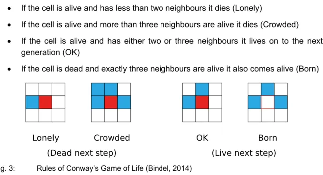
One of the simplest examples of agent-based model is Conway’s Game of Life, a two-dimensional cellular automaton invented by the mathematician John Horton Conway in 1970. A cellular automaton is a computational machine that performs actions based on certain rules. The “world” of Game of Life is a grid in which each square contains a cell that can have two states, alive or dead. The state of a cell in the next time step depends on its current state and the states of its neighbours, that is to say the 8 cells around it. The rules of the game are quite simple and are applied to each one of the cells at each time step:

 If the cell is alive and has less than two neighbours it dies (Lonely)

 If the cell is alive and more than three neighbours are alive it dies (Crowded)  If the cell is alive and has either two or three neighbours it lives on to the next

generation (OK)

 If the cell is dead and exactly three neighbours are alive it also comes alive (Born)

Fig. 3: Rules of Conway’s Game of Life (Bindel, 2014)

Game of Life can be initialised with any initial distribution, one possibility being a definition of the density of live cells, and it will evolve based on the above-mentioned rules. After the model starts running, the population of cells will constantly be changing and many

(22)

20

that is rather common in Game of Life and oscillates between three different states in a cyclical fashion: this pattern emerges from the selective pressures generated by the rule of the game.

Fig. 4: Pulsar (Wikimedia, 2007)

What is striking about this simple model is that from such simple rules hundreds of thousands of different patterns can emerge, patterns that would be impossible to predict from the rules that govern the survival of one cell. This concept continues to be valid when more complex models are considered.

2.3.3 When to use agent-based modelling

As stated in section 2.2 ABM presents several advantages over other modelling techniques like system dynamics. These advantages make ABM particularly suitable for the study of complex adaptive systems. Just like any other modelling technique, however, ABM presents both advantages and limitations and these will be briefly discussed in this section.

The main advantages are: ability to capture emergence, natural description of the system and the possibility to add heterogeneity to the model. The ability to capture emergence is intrinsic to the concept of ABM phenomena, since its concept is based on interacting entities: this makes it the best choice when the modelled system involves individual behaviour, which is ill suited to be modelled with differential equations. Individual behaviour is in fact non linear and often characterised by thresholds. Moreover emergent phenomena can be highly counterintuitive and system dynamics allows studying a phenomenon only if this is explicitly described in the differential equations: as a consequence radically new system behaviours can only be captured by agent-based modelling. Another advantage of ABM is that it provides a natural description of the system, since in real complex systems the structure is generated from the bottom up and not vice versa. This natural approach provides an easier way of implementing the model rather than trying to describe the global behaviour directly. This characteristic allows for heterogeneity in the model that cannot be included when differential equations are used. This allows for example grouping agents based on specific parameters and studying what

(23)

2 Fundamentals of agent-based simulation is the difference between innovators and early adopters when a new technology enters the market. This feature of ABM will be used in the model developed in this master thesis to group producers based on their market share and see how their decision to switch to FCVs depends on this variable.

Of course ABM presents also some disadvantages that limit its possible uses: among these are the impossibility of having a general-purpose model, the difficulty of modelling human behaviour and its computational requirement. First of all, just like any other modelling technique, an agent-based model has to answer a specific question and no ABM can exist that captures all the complexities of a given system. The model should be build with the right level of complexity to serve its purpose. Another issue regards ABMs that simulate human behaviour: since human behaviour can hardly be converted in numbers and formulas it follows that most of the times the results of ABMs can only be interpreted on a qualitative level. However, this mainly depends on the degree of accuracy of the used input data and on the expertise of the modeller, which in some cases could allow a quantitative interpretation as well. Lastly, it should be noted that ABM can be extremely computational intensive, especially if the analysed system is large and the number of agents is high. Due to the randonm initialization of agent variables and the randomness of their interactions the model needs to be run a large number of times in order to obtain statistically significant results. As a consequence, ABM often requires the use of a computer cluster to run simulations in a reasonable amount of time.

(24)

(25)

3 Model description

This chapter describes the agent-based model used in the master thesis project. After giving a general description of how the model is organised, the anatomy of the agents and the structure of their interactions are described in detail.

3.1 General structure of the model

The model implemented in this master thesis is based on (M. Schwoon, 2006). It tries to capture the main dynamics of the system made up of consumers, car manufacturers (here indicated as producers), filling stations operators and the government. This system can be interpreted as a socio-technical system: the technical subsystem includes the refuelling infrastructure and the cars, whereas the social subsystem includes all the actors indicated above.

In this model the government makes use of a policy to promote the diffusion of fuel cell vehicles: this policy is either a tax on the purchase of internal combustion engine vehicles (ICEVs) or a an equivalent subsidy for fuel cell vehicles (FCVs). Provided that this incentive to buy FCVs is high enough, consumer will start buying them and filling stations will in turn start selling hydrogen. The tick, that is the time unit in the model, represents one quarter. Every single tick the following series of events happens in the model:

 Producers choose the drivetrain technology and price for their cars that maximise a weighted average of expected income and expected sales, taking limited capital availability into account

 Total demand for cars is calculated using a simple function in which demand is inversely proportional to the average car price set by producers

 A number of consumers corresponding to the total demand is randomly drawn from the population of consumers, asked to evaluate all the cars on the market and buy the one that they consider the best choice and is still available

 Producers engage in research and development to improve their product and make it more appealing for customers

 If FCVs have been sold in this tick the hydrogen refuelling infrastructure develops and the share of filling stations that offer hydrogen increases

In order to allow comparability between products this model only focuses on the compact car segment, which makes up roughly 25% of the German car market. The choice fell on this segment because, being it the largest in the German car market, it is the most likely to generate a high enough hydrogen demand to stimulate the growth of the refuelling infrastructure. The results of the model are mainly interpreted in terms of the share of FCVs in the quarterly car sales (unless otherwise stated the share refers to the compact car segment only).

(26)

3 Model description

24

3.2 Consumers

Consumers in the model symbolise German compact car owners: each one of them owns a car and will buy a new one when randomly selected to do so. Each car is characterised by different features, represented by an array of 4 values between 0 and 1 ( ) and a boolean variable that indicates the technology of the drivetrain (FCV). A car is thus represented as

,

(1)

where FCV is 1 for fuel cell vehicles and 0 for internal combustion engine vehicles.

At the beginning the simulation all the cars in the model are ICEVs and the features array of each car is initialised with random values from a uniform distribution between 0 and 1. Although such an array cannot represent real car characteristics, it allows to create heterogeneity in consumers preferences and to model producers’ efforts to improve car features.

Each consumer is assigned a location in a simple grid, similar to that of Game of Life, in which it is surrounded by 8 neighbours. Fig. 5 shows a subset of the consumers’ grid in which a consumer, represented in blue, and its neighbours, in red, are found: the entirety of the coloured cells is called neighbourhood. This is a representation of the social network of the consumer in which neighbours represent people whose buying decisions have an effect on the consumer’s own decision, like friends, colleagues, relatives, etc. In order for all consumers to have the same number of neighbours and to avoid edge effects the grid cells are connected as to form a toroidal surface like the one shown in Fig. 6, which is common practice in spatial agent-based models.

Fig. 5: Representation of a consumer’s neighbourhood (Wikimedia, 2013)

(27)

3 Model description

3.2.1 The consumat approach

The way consumers make buying decisions in the model follows the consumat approach (Jager, 2000), a model of consumer behaviour meant to be applied to artificial consumers (the consumats). In this approach each consumat makes a buying decision based on expected utility associated to the product and the experienced uncertainty in the decision. The expected utility is in turn divided into two parts, namely a social need and a personal need. The personal need represents the personal preference for certain product features and its satisfaction depends on the difference between these preferences and the real product characteristics. The social need is related to social identity and can be formalised as having a preference for consuming the same products as the neighbours: the more neighbours consume the same product, the higher the satisfaction of the social need. The expected utility ( of a certain product j is given by

1

к (2)

where represents the personal need, the social need, the relative importance of the personal need, the price of the product and к is a scaling parameter, which states the relative weight of price. When the expected utility of a product is above a given threshold, the consumat is said to be satisfied with this product. The second part of the decision is determined by the experienced uncertainty ( ), defined as:

, , (3)

where _, is the current value of expected utility and _, is the value of the utility in previous period. The experienced uncertainty is high when there is a large variation in expected utility between two subsequent ticks. If this value is lower than a given threshold, the consumat is said to be uncertain.

In deciding what product to consume the consumat can employ different cognitive processes, based on its level of expected utility and experienced uncertainty :

 Repetition (satisfied and certain), the consumat consumes the same product as before

 Deliberation (dissatisfied and certain), the consumat evaluates the expected utility of product and chooses the one that maximises it

 Imitation (satisfied and uncertain), the consumat consumes the product with the largest share in the neighbourhood

 Social comparison (dissatisfied and uncertain), the consumat evaluates the product it was previously consuming and the one with the largest share in the neighbourhood: the one with the largest expected utility is consumed

(28)

3 Model description

26

usually agreed upon that social comparison plays an important role in the choice of a car and becomes particularly important if the consumer experiences uncertainty due to a new product like a FCV. Yet, including this cognitive process would be rather difficult in this model: this problem will be further discussed in section 6.5.1. It is important to point out however that considering social comparison would give a lower market penetration at the beginning since the consumers that do follow this cognitive process will not even consider the purchase of a FCV. Having removed the possibility for social comparison consumers will only deliberate.

3.2.2 Choice of the car

Starting from formula (2), adding the refuelling effect ( _, _, ) and using the price elasticity ( ) as a scaling parameter the total expected utility for a car is obtained. The value of total expected utility of the i-th car model for the k-th consumer is defined as follows:

, , ,

1 _, _, _, _,

, 1 ,

| | (4)

In order to choose which car buy it evaluates the total expected utility that it would get from buying each one of them and then buys the one with the highest total expected utility that is still available.

The total expected utility takes four aspects into account:

 The direct utility ( _, _, ) the consumer would derive from buying a certain car. This quantity depends on its preference about car features, described by an array of values between 0 and 1 ( _{, ,} ), in which each element corresponds to the preference about a specific car feature

, , 1

1

, , , , (5)

The value of direct utility is as close to one as the car features are close the preferences of the consumer.

 The social need ( _, _, ) reproduces the effect that neighbours’ decisions have on the decision of the consumer. This is represented by the share of cars with a certain drivetrain technology that neighbourhood would have if the deciding consumer bought a car with the same drivetrain technology.

, , ,

1

, , ,

(29)

3 Model description The higher the share of consumers that already have a car with the considered drivetrain technology, the higher the satisfaction of the social need.

The relative importance of direct utility and social need is different for each consumer to discern people that give a high importance to own opinion from the ones that tend to give more importance to the opinion of other consumers. This heterogeneity is represented in the total expected utility via the parameter : for the extreme case of 1 the consumer is not in any way influenced by its neighbours, while for 0 it completely neglects its own opinion. Since the last case is rather unlikely, a lower threshold of 0.4 is chosen for . The value of this parameter is thus randomly drawn from a uniform distribution between 0.4 and 1.  The refuelling effect _, _, takes into account the disadvantage that FCVs

would have compared to ICEVs due to a lower number of filling stations that sell hydrogen compared to conventional fuels. This is defined as

, , , 1 exp , (7)

where is the driving pattern of the consumer, _, is the share of hydrogen filling stations and is the fuel availability factor. The refuelling effect is always equal to 1 for conventional vehicles and is determined by car usage and the share of filling stations that sell hydrogen for FCVs. The driving pattern describes consumer car usage that is close to 0 for few short trips or closer to 1 for many long distant trips. The assumption here is that the importance of having a high share of hydrogen filling stations (HFSs) is higher if the consumer in reality drives often and to distant places. Fig. 7 shows how the refuelling effect varies with the share of HFSs for consumers with different driving patterns: it is clear form the chart that consumers with a high value of will have a very low refuelling effect for low shares of HFSs and are thus not likely to buy a FCV when the technology is first introduced. On the other hand, the refuelling effect has a very low impact on consumers with a low driving pattern so that they are the most likely to become early adopters of FCVs. As the share of FCVs sold in one tick increases, the amount of HFSs increases accordingly, so that consumers with high driving pattern are more and more likely to consider the purchase of a FCV.

(30)

3 Model description

28

Fig. 7: Refuelling effect with varying share of hydrogen filling stations

The importance of the share of filling stations that sell hydrogen in the refuelling effect is directly influenced by the fuel availability factor, set to be – 3 in the central case, and indirectly by the own price elasticity of the consumer

 The consumer price, at the denominator of the total expected utility function, plays an important role in the consumer decision and its importance is determined by the own price elasticity ( ), that replaces the scaling factor used in the consumat approach. Own price elasticity is a measure used in economics to show the responsiveness of demand to a change in price of a certain product and is defined as

(8)

where is the demanded quantity and is the price. To be more precise, it represents the percentage change in quantity demanded in response to a one percent change in price.

3.2.3 Change in consumer preferences

Consumer preferences are not constant, but change as the products consumers are exposed to change with time, due to the mere-exposure effect. This phenomenon, extensively studied and used in marketing, causes consumers to prefer products they are most familiar with rather than others they have never encountered before (Zajonc, 2001). This effect is taken into account in the model with a shift of preferences of all the consumers towards the characteristics of the “average car” sold in one quarter, where each feature is represented by an average across all car models sold weighted by market share. This mechanism gives an advantage to large producers, because they have a higher impact on the determination of the average car and can thus influence future consumer decisions. The preferences of each consumer are updated at the end of each tick using the following formula:

(31)

3 Model description

, , , , 1 , , ∙ , (9)

where _{, ,} is the preference for the specific feature in the current quarter, _{, ,} is the one for the next quarter, the summation represents the feature of the average car and indicates the speed at which prefereces vary. The value of is set to be 0.99, as to have a small but noticeable change during one model run.

3.3 Producers

Since producers are the main focus of this model, particular attention was given to a realistic representation of their behaviour. Each one of the producers has to make a decision at the beginning of the quarter about the price to set and the corresponding quantity of cars it expects to sell. A quarter is considered too short of a time to adjust the production capacity if the demand is higher than expected, thus the expected quantity also represents the maximum amount of cars a producer can sell in one quarter.

3.3.1 Production decision

In order to determine the optimal price for its car in one quarter every producer performs an objective function maximization, in which not only income is considered but also the expected market share. The objective function is defined as:

max 1 , _∑ , , , , ∑ _, with _, exp , ∑ , (10)

where _, is the expected income, _, is the expected sales, ∑ _, and ∑ _, are, respectively, the total income and the total sales of all producers in the previous period.

The expected income is defined as

, , , , , (11)

where _, is the price and _, ) is the variable cost per unit, which is considered constant across producers and 10% higher for FCVs compared to ICEVs. The main assumption behind this number is that all the cost reduction due to learning curves will have already been realised by the year in which the tax or subsidy is introduced. Even though this is a very strong assumption, it is necessary to keep the number of model dynamics low. Considering learning curves to take cost reductions into account is one of

(32)

3 Model description

30

(Kwasnicki & Kwasnicka, 1992) shows that producers using this function maximization in the price setting process perform better than the ones simply maximizing income. The weight function is conceived as to focus more on market share when the current producer had a low market share in the previous period and more on income in case of previously high market share. It is relatively straightforward that the two components of the objective function push the price in different directions: choosing a low price will decrease income and increase expected quantity, thus increasing the expected market share, while a high price will do exactly the opposite. In case the producer had a negative income in the previous quarter only expected income is maximised ( _, 0).

Each producer, that hasn’t switched to fuel cells yet, performs an optimization of the objective function at each tick for both ICEVs and FCVs, and decides to switch to FCVs as soon as the maximum value of the objective function is higher for FCVs. Since switching the whole production to FCVs is expensive and the production line needs to be adapted to the new drivetrain technology, producers that make the switch cannot go back to producing ICEVs.

3.3.2 Expected quantity estimation for a given price

The estimation of the expected quantity _, corresponding to a specific price _, is done by the producers in four steps.

First of all each producer evaluates how competitive its car is compared to the average car on the market in the previous period (at the end of the previous tick the car of the current producer has been improved with R&D): to do so it tries to replicate the way consumers evaluate the total expected utility of cars using known variables available from its customers and publicly available data (e.g. car features, market shares).

The variable is called competitiveness ( _, ) and is defined as follows:

, ̅ ₁ _∆ ₁ ̅ _, _, _, , 1 , | | with ∆ ∑ _{, ,} ∑ _{, ,} ∙ _, _, (12)

where ∆ is the sum of the differences between the features of the producer’s car model and the weighted average features on the market. The social need and the refuelling effect are estimated using the accessible information. Producers know the driving patterns of their customers from maintenance records and use its average value to estimate the refuelling effect. As regards the social need, this is estimated using the total number of existing FCVs and the total number of vehicles owned by the consumers, thus obtaining an “average density” of FCVs in the neighbourhood of every consumer. This approach is a little bit different from the one used in (M. Schwoon, 2006), where the estimation is made assuming that the share of FCVs sold in the previous period can also be found in the individual customer’s neighbourhood. This approach is somewhat unrealistic since, on

(33)

3 Model description average, a new car is bought in a specific neighbour only once every 10 quarters and thus the share of FCVs in the specific neighbourhood will always be lagging the share of FCVs in the newly registered cars. The result would be that producers always overestimate the share of FCVs in the average neighbourhood and might erroneously decide to switch when this is not yet convenient for them.

Knowing the competitiveness of its own product, the producer can use it to determine how its market share will change in the current tick compared to the last one. To do this it has to compare this value with the average competitiveness of all producers, to determine whether it is below or above average.

The average competitiveness is referred to the cars sold in the previous tick and is computed as follows

̅_, _, _, (13)

Since the current producer has no access to the driving pattern of the other producers’ customers, the estimation of the refuelling effect is done using the average driving pattern of own customers. This means that the estimated average competitiveness will be different for each one of the producers.

Assuming that the change in average competitiveness of this period will be equivalent to the one observed in the last tick we have

̅_, ̅_, ̅_, ̅_, ̅, ̅_, , (14)

The estimated average competitiveness depends on the decision of the current producer and is computed as

̅_, _, ̅,

, 1 , , ,

(15)

Finally the new market share can be estimated comparing own competitiveness with the average competitiveness.

, , _̅ ,

, ,

(16)

In order to obtain the expected quantity from the expected market share the total demand needs to be estimated. This is done assuming that the size of the market is constant (no market growth with time) and that the total demand decreases when the weighted after tax average price of cars increases, and extent to which this happens is taken into account by the elasticity of demand of the whole market segment ( .

(34)

3 Model description

32

̅_, ̅

̅ 1 , , 1 , , (17)

and then the total demand is estimated

,

̅_, (18)

where is the size of the market in monetary terms. Now that the total demand and the estimated market share are available, the expected quantity can be easily computed as

, , , (19)

It should be noted that producers with a higher market share can better predict the number of sales in the certain period due to their higher impact on the average price and average competitiveness.

In last step of the production decision process the producer verifies whether it has enough capital to produce an amount of cars equal to the expected quantity. The required amount of capital is given by

, , (20)

where is the productivity of capital, that is to say the number of products that is possible to produce with a unit of physical capital. When a producer switches to FCVs the productivity of capital decreases by 25%, so that the number of cars that is possible to producer after the switch without a capital expansion also decreases by 25%. If the required capital is higher than the available capital the producer can access the capital market and expand the production capacity through investments, which are limited to 30% of the currently available capital. If the capital is still not enough after the investment the expected quantity will be limited to the maximum amount of cars that it is possible to produce with the current capital plus investment, thus

, ∙ , (21)

For a more detailed description of the adjustment of capital stock refer to (M. Schwoon, 2006).

A visual representation of the objective function is given in Fig. 8 for producers with different market shares in the previous quarter. In the left part of the plot the value of the objective function increases with increasing price due to increasing expected income, while in the right part it decreases as a result of decreasing expected quantity. With the

(35)

3 Model description optimization process the producer chooses the price to which the maximum value of the function is associated, that is higher for producers with a higher market share, since income has for them a higher weight in the objective function. The value of the function is also higher for higher market share because the expected quantity is higher in this case.

Fig. 8: Objective function value with varying price

3.3.3 Research and Development

After the selected consumers have bought a car the producers try to improve their product so that its features will be more appealing to potential customers in the next quarter. They cannot observe consumer preferences directly, but the characteristics of the cars sold in this quarter are readily available and with these the features of the “average car”. Because producers are aware of the mere exposure effect, with which preferences shift towards the average car, they will try to change the features of their car models so that they get closer to those of the average car. Since not all the features can be improved at once, producers focus on the farthest and closest to the average car respectively, as to both maintain its advantages and reduce its major shortcomings.

It is rather difficult to determine the success of the research and development process, but it stands to reason that the probability of improving the design of the product should increases if the producer invests more money in these activities. The R&D expenditures of one producers at time are a fixed fraction of the capital

, , (22)

where is set to 0,12%. The improvement of the two features on which research and development focus is computed as

(36)

3 Model description 34 , 1 , , , , , ∙ , with _, 1 ∙ , (23)

where and are non-negative parameters and is a random value drawn from a uniform distribution between 0 and 1. As it can be seen from the formula, the likelihood of improving a specific feature increases when the R&D expenditures increase.

3.4 Match of supply and demand

After all the producers have made their decision about price and production quantity total demand is estimated with the formulas

̅

with ̅ ∑ _, 1 , ,

(24)

where ̅ is an average of the after tax price across all producers weighted by market share in the previous tick. It is assumed that the total demand varies based on the average price and represents the number of consumer willing to buy a car at this price level. A number of consumers corresponding to is randomly drawn from the population and each one of them pre-orders a car based on total expected utility and availability. The production of cars happens only after the consumer order, so that producers that overestimate sales will not lose variable costs but have the only disadvantage of a production capacity that is higher than needed. On the other hand they cannot increase the production capacity if the demand is higher than expected, thus implying an opportunity cost. In case the car with the highest total expected utility for a given consumer is not available anymore, it tries to buy the second-best car, and may end up buying the least preferred car if this is the only one left. This behaviour is rather unrealistic, but the alternative would be a stock of unsold cars for every producer that needs to be sold in the next tick: these cars would have features that are almost identical to the ones of the new car and would have to be sold at a different price. This simple approach is chosen to avoid a substantial increase in the complexity of the model.

3.5 Hydrogen refuelling infrastructure

Three different infrastructure scenarios are considered in the model: no exogenous infrastructure, exogenous infrastructure and high exogenous infrastructure. In the case of no exogenous infrastructure, there is no planned growth and the share of hydrogen filling stations (HFSs) increases only in response to an increase in the share of FCVs in the quarterly sales in the whole car market. In the case of exogenous growth, a fixed amount

(37)

3 Model description of HFSs is added every quarter, with a fixed 0.15% and 0.3% growth of the share for the cases of exogenous growth and high exogenous growth respectively.

In order to limit the complexity of the model filling stations are not represent as agents, but a general behaviour of the whole infrastructure is assumed. Although no differential equations are used, this is a top-down approach conceptually similar to system dynamics. For all three scenarios, the feedback of the hydrogen infrastructure can be described as follows:

 if the share of FCVs in the cars sold in one period is higher than the share HFSs, the infrastructure grows by the highest amount technologically feasible (

),

equal to 1.5%

 if the share of FCVs in the total market is higher than 20%, the infrastructure grows as fast as possible until full coverage is reached

 otherwise the new share of HFSs is given by the formula

, ,

min

,

, , (25)

where _, is the maximum share of FCVs in the car sold up to tick t, _,

the

one up to the tick before, represents the impact of the growth of the share of FCVs on the infrastructure and

the extent of exogenous growth. This means

that the growth of the infrastructure will accelerate if the FCV share reaches a new maximum.

is set to be 1.5 in the central case, as to give an increase in the share

of HFSs 50% higher than the increase in the share of FCVs that causes it. It should be noted that the share of FCVs considered for the development of the hydrogen infrastructure is the one in the whole car market: since the considered market segment represent roughly 25% of it, the share used here is obtained by multiplying the share of sold FCVs in the segment by 0.25.

(38)