Computing primal solutions with exact arithmetics in SCIP.

Alma Mater Studiorum

Universit`

a di Bologna

SCUOLA DI INGEGNERIA E ARCHITETTURA

Corso di Laurea Magistrale in Ingegneria dell’Automazione

TESI DI LAUREA

in

Optimization Models and Algorithms

Computing Primal Solutions

with exact arithmetics in SCIP

CANDIDATO :

Luca Fabbri

RELATORE :

Prof. Andrea Lodi

CORRELATORI :

Prof. Enrico Malaguti

Dr. Ambros Gleixner

III Sessione

Sommario

La ricerca di soluzioni esatte per problemi misti interi `e un tema molto attuale all’interno della comunit`a scientifica. I risolutori MIP allo stato dell’arte utilizzano una rappresentazione numerica in formato floating-point, introducendo quindi approssimazioni. Sebbene tali risolutori di problemi misti interi forniscano risultati affidabili per la maggior parte dei problemi, ci sono casi in cui `e necessaria una maggiore precisione. `E noto, infatti, che per alcune applicazioni i risolutori floating-point restituiscano soluzioni errate, vale a dire soluzioni indicate come accettabili a causa delle approssimazioni, le quali non supererebbero un controllo con aritmetica esatta e non possono essere implementate nella pratica.

L’ambito in cui questa tesi `e stata sviluppata `e SCIP, un risolutore di programmi interi misti, sviluppato presso lo Zuse Institute di Berlino. In tale sede abbiamo considerato un nuovo approccio per risolvere problemi misti interi in modo esatto. In particolare abbiamo sviluppato un plugin -un gestore di vincoli da inserire in SCIP - al fine di analizzare la precisione delle soluzioni floating-point ottenute e calcolare soluzioni primali esatte a partire da tali soluzioni floating-point.

Abbiamo condotto alcuni esperimenti computazionali per testare il ge-store di vincoli per soluzioni primali esatte, attraverso l’utilizzo di due principali configurazioni: la modalit`a di analisi e la modalit`a di applicazione. La modalit`a di analisi ha permesso di raccogliere statistiche riguardanti l’attuale affidabilit`a di SCIP. I risultati hanno confermato che le soluzioni cos`ı ottenute sono sufficientemente accurate per un larga parte delle istanze. Tuttavia, la nostra analisi evidenzia anche la presenza di errori numerici aventi entit`a variabile. Utilizzando la modalit`a di applicazione, il gestore di vincoli suggerisce soluzioni esatte a partire dalla parte intera delle soluzioni floating-point. In tale configurazione abbiamo rilevato un generale migliora-mento della qualit`a delle soluzioni finali trovate, senza tuttavia sopperire ad un significativo calo nelle prestazioni.

Abstract

The research for exact solutions of mixed integer problems is an active topic in the scientific community. State-of-the-art MIP solvers exploit a floating-point numerical representation, therefore introducing small approximations. Although such MIP solvers yield reliable results for the majority of problems, there are cases in which a higher accuracy is required. Indeed, it is known that for some applications floating-point solvers provide falsely feasible solutions, i.e. solutions marked as feasible because of approximations that would not pass a check with exact arithmetic and cannot be practically implemented.

The framework of the current dissertation is SCIP, a mixed integer programs solver mainly developed at Zuse Institute Berlin. In the same site we considered a new approach for exactly solving MIPs. Specifically, we developed a constraint handler to plug into SCIP, with the aim to analyze the accuracy of provided floating-point solutions and compute exact primal solutions starting from floating-point ones.

We conducted a few computational experiments to test the exact primal constraint handler through the adoption of two main settings. Analysis mode allowed to collect statistics about current SCIP solutions’ reliability. Our results confirm that floating-point solutions are accurate enough with respect to many instances. However, our analysis highlighted the presence of numerical errors of variable entity. By using the enforce mode, our constraint handler is able to suggest exact solutions starting from the integer part of a floating-point solution. With the latter setting, results show a general improvement of the quality of provided final solutions, without a significant loss of performances.

Acknowledgements

This text is the last stage of a long journey. I did not walk alone, that’s why I need to thank some people.

My experience in Berlin has been intense and gave me a personal and professional growth. I would like to express my sincere gratitude to Ambros Gleixner for teaching me a lot with his knowledges and his example, and for his support. Thank you Anna for the good time spent at ZIB and for your friendship. I would like to thank all the other ZIB guys that helped me, as well as Berlin itself to be so inspiring.

A special thank also to my supervisor, Professor Andrea Lodi, who gave me this opportunity and always let me feel his support and faith.

Colgo questa occasione per ringraziare chi mi ha sempre sostenuto in questi anni di studio e di vita. Non pu´o mancare un grazie ai miei amici Guido, Silvia e Marche, che hanno condiviso con me i loro spazi e il loro tempo. Le nostre esperienze e l’affetto che mi avete dato saranno sempre con me. Grazie anche a Gardo e Sonia per la loro grande e preziosa amicizia.

Un grazie immenso a Simona, per aver condiviso quotidianamente tutti i miei sforzi, riuscendo sempre a spronarmi con amore. Grazie per il tuo sostegno insostituibile e spontaneo, e anche per aver contribuito a questa tesi con la tua penna rossa sul mio inglese.

Il ringraziamento finale va alla mia famiglia. A partire dai miei nonni, nei quali vedo riflesso il mio passato, e dai quali ricevo incondizionato affetto. Grazie ad Annalisa, una sorella incredibile, che fra le tante cose mi ha accompagnato nei primi difficili passi a Berlino. Sei un grande riferimento per me. Grazie a Patrizia e Achille, i miei genitori. Custodisco gelosamente tutto quello che mi avete dato e la vostra fiducia totale, che mi ha sempre sorretto. Questo risultato lo dedico a voi.

Contents

1 Floating-point Constraint Integer Programming 9

1.1 From Mathematical Programming to CIP . . . 9

1.1.1 Mathematical Programming . . . 9

1.1.2 Linear Program . . . 11

1.1.3 Integer (Linear) Program . . . 11

1.1.4 Mixed Integer (Linear) Program . . . 12

1.1.5 Constraint Program . . . 13

1.1.6 Satisfiability Problems . . . 14

1.1.7 Comparing MIPs, CPs and SAT . . . 14

1.1.8 Constraint Integer Program . . . 15

1.2 Standard solution algorithms . . . 16

1.2.1 Branch and Bound . . . 16

1.2.2 Cutting planes . . . 17

1.2.3 Branch and cut . . . 18

1.3 Floating point arithmetic . . . 19

1.3.1 Floating point representation . . . 19

1.3.2 Definition of feasibility and optimality . . . 20

1.3.3 Floating point arithmetic and tolerances for MIP solvers 22 2 SCIP: Solving Constraint Integer Programs 25 2.1 Introduction to SCIP . . . 25

2.1.1 What is SCIP . . . 25

2.1.2 History and performances . . . 26

2.1.3 Features . . . 28

2.2 Working with SCIP . . . 29

2.2.1 Code structure and documentation . . . 29

2.2.2 File system organization . . . 30

2.3 Constraint Handlers . . . 31

2.3.1 Role of constraint handlers . . . 31

2.4.1 QSopt ex . . . 33

2.4.2 Iterative refinement . . . 34

3 Xprim Constraint Handler 35 3.1 Aim and motivation . . . 35

3.1.1 Dangers of numerical computation . . . 35

3.1.2 Wireless Network Design Problem . . . 36

3.1.3 Advances in exact MIP solving . . . 37

3.1.4 Integer and continuous parts of a solution . . . 38

3.2 Tool description . . . 39

3.2.1 Analysis and enforce modes . . . 39

3.2.2 Initialization . . . 39 3.2.3 Algorithm . . . 40 3.2.4 Tolerances . . . 42 3.3 Implementation details . . . 42 3.3.1 Properties . . . 43 3.3.2 Additional parameters . . . 44 3.3.3 Data structures . . . 45 3.3.4 Interface methods . . . 47 3.3.5 Callback methods . . . 47 3.3.6 GMP Library . . . 49 4 Computational experiments 51 4.1 Instances . . . 51 4.2 Analysis mode . . . 52 4.2.1 Tables . . . 52 4.2.2 Results . . . 54 4.3 Enforce mode . . . 59 4.3.1 Tables . . . 59 4.3.2 Results . . . 59 4.4 Conclusions . . . 65 List of Figures 67 List of Tables 68

Chapter 1

Floating-point Constraint

Integer Programming

In this chapter an overview of the topic we are going to explore is given. In section 1.1 we start from the definition of Mathematical Program, going through many different optimization models under different restrictions. The final model we want to obtain is Constraint Integer Programming, a quite general concept SCIP is based on.

In section 1.2 the main algorithms used in solving optimization problems are presented. In particular, original branch-and-bound and cutting planes are described. Nevertheless, it is worth to consider that state-of-the-art solvers use more sophisticated algorithms derived from these techniques.

In section 1.3 we discuss floating-point arithmetic, by considering how numbers are represented in a calculator, as well as advantages and disadvan-tages of such representations and how to deal with issues that may arise in solving optimization problems with floating-point data.

1.1

From Mathematical Programming to CIP

1.1.1

Mathematical Programming

Mathematical programming is the use of mathematical models to assist in taking decisions. In particular it makes use of optimization models with the aim to obtain the best solution of the problem associated with the mathe-matical model. Mathemathe-matical programming is more restrictive compared to other techniques (e.g., statistics, simulation, forecasting) because of its ambition to find out the optimal solution of a problem.

For a given problem it is possible to build an associated mathematical model. Since the model is an abstraction of the problem, it has some degree of approximation compared to the real-world problem. A few optimization algorithms is then applied to the model in order to find out the best solution depending on certain criteria. It is therefore possible to provide a definition of mathematical programming as follows.

Definition 1.1 (Mathematical Program). Given n decision variables x1, x2, . . . , xn, an objective function f (x1, x2, . . . , xn), and m constraints

gi(x1, x2, . . . , xn) ≤ bi, i = 1, 2, . . . , m, a mathematical program is to solve

z∗ = min f (x1, x2, . . . , xn)

gi(x1, x2, . . . , xn) ≤ bi i = 1, 2, . . . , m

xj ≥ 0 j = 1, 2, . . . , n

(1.1)

The optimal solution is given by the set of values x∗₁, x∗₂, . . . , x∗_n for decision variables such that z∗ = f (x∗₁, x∗₂, . . . , x∗_n).

The mathematical model has to be built considering two opposite re-quirements. It is important to have a model as faithful as possible to the real-world problem. In fact the solution found is optimal for the built model, but it is not necessarily optimal for the real-world problem. The quality of the optimal solution is then strictly correlated to the quality of the model. On the other side, a model very close to reality is likely to be complex, and consequently harder to be solved.

In practice, mathematical models in the general form (1.1) are usually not solvable by state of the art algorithms within acceptable time. It is therefore necessary to introduce some limitations to the model in order to obtain models easier to solve, by avoiding to lose sufficient closeness to real-world problems.

It is possible to introduce a classification of the models. First, we can distinguish between linear programming and nonlinear programming. A linear program is a mathematical program where both objective function f (x) and constraints gi(x), (i = 1, 2, . . . , m) are all linear functions. A

Nonlinear Program is a mathematical program where at least one of such functions is nonlinear. Linear programs are clearly simpler and easier to solve.

Another classification can be done depending on the decision variables domain. If all the variables are continuous, i.e. they can have any value

1.1 From Mathematical Programming to CIP 11

within a given interval, we have a continuous problem. If variables are discrete they can only have a finite number of possible values and they define a combinatorial problem. Mixed problems contains both continuous and discrete variables.

In the following paragraphs we will go deeper into the definition of many different models.

1.1.2

Linear Program

A Linear Program has linear objective function and constraints, and conti-nuous variables.

Definition 1.2 (Linear Program). Given a matrix A ∈ Rm×n_{, vectors}

b ∈ Rm_{, a vector c ∈ R}n_{, and a vector x ∈ R}n _{of variables or unknowns, the}

linear program (LP) is to solve

z∗ = min cTx Ax ≤ b x ≥ 0

(1.2)

where m represents the number of constraints and n represents the number of variables.

The inequalities Ax ≤ b and x ≥ 0 are the constraints which specify a convex polytope over which the objective function is to be optimized.

Linear Programs are solvable in polynomial time, which was first shown by Khatchiyan [22], by using the so-called ellipsoid method. However, the mainly used method to solve linear programs is simplex algorithm, invented by Dantzig [11]. Simplex algorithm is computationally exponential, but has good performances in the mean case.

1.1.3

Integer (Linear) Program

When all the decision variables x are restricted to be integer values, we have an integer linear program.

Definition 1.3 (Integer (Linear) Program). Given a matrix A ∈ Rm×n, vectors b ∈ Rm, a vector c ∈ Rn, and a vector x ∈ Rn of variables or

unknowns, the integer (linear) program (IP) is to solve

z∗ = min cTx Ax ≤ b

x ≥ 0, _{x ∈ Z}

(1.3)

Since it is a combinatorial problem, it can, in principle, be solved by complete enumeration, which consists in considering all the possible combi-nation of the n decisional variables. Then all the constraints are checked for each combination and the objective function value is computed. The combination providing the best objective value is the optimal solution.

In practice, complete enumeration is not used because the cost would increase exponentially with the number of variables and, consequently, it would be impossible to obtain a solution within acceptable time.

1.1.4

Mixed Integer (Linear) Program

If only a subset of the variables are integer, we have a Mixed Integer (Linear) Program.

Definition 1.4 (Mixed Integer (Linear) Program). Given a matrix A ∈ Rm×n, vectors b ∈ Rm, a vector c ∈ Rn, a vector x ∈ Rn of variables or unknowns, and a subset I ⊂ N = {1, . . . , n}, the mixed integer (linear) program (MIP) is to solve

z∗ = min cTx Ax ≤ b

x ≥ 0, xj ∈ Z ∀j ∈ I

(1.4)

The vectors in the set XM IP = {x ∈ Rn| Ax ≤ b, xj ∈ Z ∀j ∈ I} are

called feasible solutions of MIP. A feasible solution x∗ ∈ XM IP is called

optimal if its objective value satisfies cTx∗ = z∗. MIP solvers usually treat simple bound constraints lj ≤ xj ≤ uj, with lj, uj ∈ R ∪ {±∞} separately

from the remaining constraints. In particular, integer variables with bounds 0 ≤ xj ≤ 1 play a special role in the solving algorithms and are a very

important tool to model yes/no decisions.

1.1 From Mathematical Programming to CIP 13

integer program its LP relaxation is defined as

ˇ

z = min cTx Ax ≤ b x ≥ 0

(1.5)

XLP = {x ∈ Rn| Ax ≤ b} is the set of feasible solutions of the LP

relaxation. An LP-feasible solution ˇx ∈ XLP is called LP-optimal if cTx = ˇˇ z.

The LP relaxation can be strengthened by cutting planes which use the LP information and the integrality restrictions to derive valid inequalities that cut off the solution of the current LP relaxation without removing integral solutions. The objective value ˇz of the LP relaxation provides a lower bound for the whole sub-tree, and if this bound is not smaller than the value ˇz = cT_{x of the current best primal solution ˇˇ x, the node and its sub-tree}

can be discarded. The LP relaxation usually gives a much stronger bound than the one that is provided by simple dual propagation of CP solvers. The solution of the LP relaxation usually requires much more time, however.

The most important ingredients of an MIP solver implementation are a fast and numerically stable LP solver, cutting plane separators, primal heuristics and presolving algorithms. Additionally, the applied branching rule is of major importance [1].

1.1.5

Constraint Program

A more general approach consists in constraint programs.

Definition 1.6 (Constraint Program). A constraint program consists of solving

f∗ = min {f (x) | x ∈ D, C(x)} (1.6) with the set of domains D = D1 × . . . × Dn, the constraint set C =

{C1, . . . , Cm}, and an objective function f : D → R.

We denote the set of feasible solutions by XCP = {x | x ∈ D, C(x)}. A

CP where all domains are finite is called a finite domain constraint program (CP(FD)). The key element for solving constraint programs in practice is the efficient implementation of domain propagation algorithms, which exploit the structure of the involved constraints. To solve a CP(FD), the problem is recursively split into smaller subproblems (usually by splitting a single variable’s domain), thereby creating a branching tree and implicitly

enumerating all potential solutions. At each subproblem (i.e., node in the tree) domain propagation is performed to exclude further values from the variables’ domains. If every variable’s domain is reduced to a single value, a new primal solution is found. If any of the variables’ domains becomes empty, the subproblem is discarded and a different leaf of the current branching tree is selected to continue the search [1].

1.1.6

Satisfiability Problems

The satisfiability problem (SAT) is defined as follows. The boolean truth values false and true are identified with the values 0 and 1, respectively, and boolean formulas are evaluated correspondingly.

Definition 1.7 (Satisfiability Problem). Let C = C1∧ · · · ∧ Cm be a

logic formula in conjunctive normal form (CNF) on boolean variables x1, . . . , xn. Each clause Ci = li1∨ · · · ∨ lik1 is a disjunction of literals. A

literal l ∈ L = {x1, . . . , xn, x1, . . . , xn} is either a variable xj or the negation

of a variable xj. The task of the satisfiability problem is to either find

an assignment x∗ ∈ {0, 1}n_{, such that the formula C is satisfied, i.e., each}

clause Ci evaluates to 1, or to conclude that C is unsatisfiable, i.e., for all

x ∈ {0, 1}n at least one Ci evaluates to 0.

1.1.7

Comparing MIPs, CPs and SAT

Most solvers for constraint programs, satisfiability problems and mixed inte-ger programs share the idea of dividing the problem into smaller subproblems and implicitly enumerating all potential solutions. They differ, however, in the way of processing the subproblems.

Because MIP is a very specific case of CP, MIP solvers can apply advanced problem specific algorithms that operate on the subproblem as a whole. In particular, they use the simplex algorithm to solve the LP relaxations, and cutting plane separators. In contrast, due to the unrestricted definition of CPs, CP solvers cannot take such a global perspective, but they have to rely on the constraint propagators, each of them exploiting the structure of a single constraint class. An advantage of CP is, however, the possibility to model the problem more directly, using very expressive constraints which contain a lot of structure. Transforming those constraints into linear inequalities can conceal their structure from a MIP solver, and therefore lessen the solver’s

1.1 From Mathematical Programming to CIP 15

MIP linear objective function linear constraints

real and integer variables CP arbitrary objective function

arbitrary constraints

arbitrary (discrete) variables CIP linear objective function

arbitrary constraints real and integer variables

after fixing all integer variables CIP becomes an LP Table 1.1: Comparison between MIP, CP and CIP

ability to draw valuable conclusions about the instance or to make the right decisions during the search.

SAT is also a very specific case of CP with only one type of constraints. SAT solvers mainly exploit the special problem structure to speed up the domain propagation algorithm and to improve the underlying data structures.

1.1.8

Constraint Integer Program

Constraint integer programs allow to merge CP, SAT and MIP techniques, by combining their advantages and compensating for their individual weak-nesses.

Definition 1.8 (Constraint Integer Program). A constraint integer program consists of solving

c∗ = {min cT_{x | C(x) ∈ R}n, xj ∈ Z ∀j ∈ I} (1.7)

with a finite set C = {C1, . . . , Cm} of constraints Ci: Rn → {0, 1}, i =

1, . . . , m, a subset I ⊂ N = {1, . . . , n} of the variable index set, and an objective function vector c ∈ Rn.

A CIP has to fulfill the following condition:

∀ ˆxI ∈ ZI∃ (A0, b0) : {xC ∈ RC| C( ˆxI, xc)} = {xC ∈ RC| A0xC ≤ b0} (1.8)

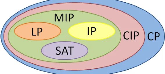
Figure 1.1: Outline of mathematical programs under different restrictions.

Restriction 1.8 ensures that the remaining subproblem, after integer variables have been fixed, is always a linear program. This means that in the case of finite domain integer variables, the problem can be, in principle, completely solved by enumerating all values of the integer variables and solving the corresponding LPs. Note that this does not forbid quadratic or even more involved expressions. Only the remaining part after fixing (and thus eliminating) the integer variables must be linear in the continuous variables.

1.2

Standard solution algorithms

1.2.1

Branch and Bound

The branch-and-bound procedure is a very general and widely used method to solve optimization problems. The key idea is to successively divide the given problem instance into smaller subproblems until the individual subproblems are easy to solve. The best among the subproblems’ solutions is the global optimum.

Figure 1.2 show the fundamental steps of branch-and-bound algorithm. The splitting of a subproblem into two or more smaller subproblems in step 7 is called branching. During the course of the algorithm, a branching tree is created with each node representing one of the subproblems. The root of the tree corresponds to the initial problem R, while the leaves are either “easy” subproblems which have already been solved or subproblems in L which still

1.2 Standard solution algorithms 17

Figure 1.2: Branch-and-bound algorithm [1].

have to be processed. The intention of the bounding in step 5 is to avoid a complete enumeration of all potential solutions of R, which are usually exponentially many. In order for bounding to be effective, good lower (dual) bounds ˇx and upper (primal) bounds ˇc must be available. Lower bounds are calculated with the help of a relaxation Qrelax which should be easy to

solve. Upper bounds can be found during the branch-and-bound algorithm in step 6, but they can also be generated by primal heuristics. The node selection in step 3 and the branching scheme in step 7 determine important decisions of a branch-and-bound algorithm that should be tailored to the given problem class. Both of them have a major impact on how early good primal solutions can be found in step 6 and how fast the lower bounds of open subproblems in L increase. They influence the bounding in step 5, which should cut off subproblems as early as possible and thereby prune large parts of the search tree. Even more important for a branch-and-bound algorithm to be effective is the type of relaxation that is solved in step 4. A reasonable relaxation must fulfill two usually opposite requirements: it should be easy to solve and it should yield strong dual bounds. In Mixed Integer Programming the most widely used relaxation is the LP relaxation, which proved to be very successful in practice.

1.2.2

Cutting planes

Besides splitting the current subproblem Q into two or more easier sub-problems by branching, while solving MIPs one can also try to tighten the

Figure 1.3: Branching on a single fractional variable [1].

Figure 1.4: A cutting plane that separates the fractional LP solution ˇx from the convex hull QI of integer points of Q [1].

subproblem’s relaxation in order to rule out the current solution ˇx and to obtain a different one.

The LP relaxation can be tightened by introducing additional linear constraints aT_{x ≤ b that are violated by the current LP solution ˇx but}

do not cut off feasible solutions from Q. Thus, the current solution ˇx is separated from the convex hull of integer solutions QI by the cutting plane

aTx ≤ b.

1.2.3

Branch and cut

Branch and cut is one of the most successful algorithm that implements both and-bound and cutting planes. The problem is solved with branch-and-bound, but the LP relaxations QLP of all subproblems Q (including the

1.3 Floating point arithmetic 19

initial problem R) might be strengthened by cutting planes. In this case one has to distinguish between globally valid cuts and cuts that are only valid in a local part of the branch-and-bound search tree, i.e., cuts which were deduced by taking the branching decisions into account. Globally valid cuts can be used for all subproblems during the course of the algorithm, but local cuts have to be removed from the LP relaxation after the search leaves the subtree they are valid for.

1.3

Floating point arithmetic

1.3.1

Floating point representation

In this section we will focus on some issues related to the data implementation of problems described in section 1.1 and the algorithms described in section 1.2. We will consider how data is represented in a computer and what descends from this representation.

The main limitation is the necessity of a finite representation. This is due to both the limited capacity of the memory and to the indefinitely large runtime that would be necessary to perform computations with indefinitely large numbers. Several different representations of real numbers have been proposed, but the most widely used is the floating-point representation. This representation is composed by three different parts: sign, significand and exponent. A generic number can therefore be written as ± signif icand × baseexponent_{. Since numbers implementation is binary, usually a base equals}

to 2 is used.

In the application we are going to discuss in this thesis the double-precision floating-point numeric format is the standard way to represent numbers. This format exploits 64 bits to represent each number. In particu-lar, one bit is used for the sign, 11 bits for the exponent and 52 bits for the significand (see Figure 1.5).

The significand has an implicit integer bit of value 1. With the 52 bits of the fraction significand appearing in the memory format, the total precision is therefore 53 bits (approximately 16 decimal digits, since 53 log₁₀2 ≈ 15.955).

The most common reason why a real number might not be exactly representable as a floating-point number is when a rational number, i.e. a number having a finite representation with base 10, has an infinite binary representation. It is the case, for instance, of the decimal number 0.6. Its

Figure 1.5: Double-precision floating-point format [33].

binary representation is

0.6(10) = 0.1001(2). (1.9)

Thus, when base = 2, the number 0.6 lies strictly between two floating-point numbers and is exactly representable by neither of them. [19]

Double-precision floating-point format is widespread because of its com-putational efficiency and results obtained by floating-point computation are accurate enough for most scientific applications. Furthermore, many high precision floating-point algorithm has been developed in order to obtain an arbitrary precise computation.

Nevertheless, for some applications this is not sufficient to get reliable results. Before going deeper into this topic it is necessary to provide some other definitions.

1.3.2

Definition of feasibility and optimality

An optimization problem can be solved either for feasibility or for optimality. When feasibility only is required, the solver is asked to return an answer to the question: does it exist a feasible solution for the problem? The answer is “yes” if at least one feasible solution is found, “no” if infeasibility is proved. The goal of the solver is to find out feasible solutions and, at the end, the optimal solution.

Optimality is more challenging to achieve. In this case the objective function is considered and the goal of the solver is to return the optimal solution. Obviously, the optimal solution exists only if the problem is feasible. The optimal solution will be chosen from the set of all the feasible solutions of the problem.

1.3 Floating point arithmetic 21

Feasibility

The constraints of a MIP define a feasibility region. A solution is said to be feasible if it belongs to the feasibility region. Graphically, the feasibility region can be represented by a set of points in Rn_{, where every point}

represents a feasible solution.

For LPs the feasibility region can always be represented by a convex polytope. In this case we have a continuous region and, therefore, infinitely many solutions, except for special cases where no solutions or a single solution occur.

In case we have an IP, a convex polytope is still defined by problem constraints, but also integrality has to be taken into account. The feasible region is represented by all integral points included in the polytope. If the problem is bounded, the number of feasible solutions is finite.

In practice, feasibility is proven by checking whether a given solution satisfies all the problem constraints.

Optimality

In order to declare that a certain solution is the optimal solution, it is necessary to find some optimality conditions that will provide stopping criteria in an algorithm for MIP. The ”naive” but nonetheless important reply is that we need to find a lower bound z ≤ z and an upper bound z ≥ z such that z = z = z. Practically, this means that any algorithm will find a decreasing sequence

z1 > z2 > · · · > zs≥ z (1.10)

of upper bounds, and an increasing sequence

z1 < z2 < · · · < zt ≤ z (1.11)

of lower bounds, and stop when

zs− zt≤ ε (1.12)

where ε is some suitably chosen small non-negative value. Thus, it is necessary to find ways of deriving such upper and lower bounds.

Primal bounds Every feasible solution ˆx ∈ X provides a lower bound z = c(ˆx) ≤ z. This is essentially the only way we know to obtain lower

bounds. For some IP problems, finding feasible solutions is easy, and the real question is how to find good solutions. For other IPs, finding feasible solutions may be very difficult.

Dual bounds Finding upper bounds for a maximization problem (or lower bounds for a minimization problem) raises a different challenge. The most important approach is by relaxation, the idea being to replace a ”difficult” max (min) IP by a simpler optimization problem whose optimal value is at least as large (small) as z. For the relaxed problem to have this property, there are two obvious possibilities:

• to enlarge the set of feasible solutions so that one optimizes over a larger set;

• to replace the max (min) objective function by a function that has the same or a larger (smaller) value everywhere.

1.3.3

Floating point arithmetic and tolerances for MIP

solvers

Most MIP solvers are based on floating-point arithmetic and work with tolerances to check solutions for feasibility and to decide on optimality. In their feasibility tests, solvers typically consider absolute tolerances for the integrality constraints and relative ones for linear constraints. Some of them normalize the activity of linear constraints individually, others scale directly the constraint matrix.

The tolerances affect solution times and solution accuracy, normally in opposite ways, and the solvers apply different strategies here. Typically it can happen that for a given instance different solvers compute different optimal objective values. If one fixes all integer variables from the reported solution to the closest integer value and recomputes the continuous variables by solving the resulting LP with exact arithmetic, some of these post-processed solutions turn out to be infeasible compared to exact arithmetic and zero tolerances.

It is worth to note that this does not mean that any of the solvers made a mistake. It only means that the computed solution lies outside the feasible area described by the input file, but inside the extended feasible area created by reading in the problem and introducing tolerances. It is only solutions that are feasible in the latter sense that solvers attempt to deliver, and those

1.3 Floating point arithmetic 23

are the solutions the checker checks. More precisely, the operation which rounds the reported value of the integer variables to the closest integer is only applied to compute fully reliable primal bounds for the MIPs.

As introduced in section 1.3.1, floating-point computations can be per-formed quickly on computers but the limited size of this representation has its disadvantages. The error incurred by a single operation is usually small but algorithms requiring many operations may accumulate and propagate these small errors, leading to errors of significant magnitude.

Let’s now consider the phases of the process that precedes the actual solution of the problem.

The MPS file format, which is used as a standard to define MIP instances, requires the input numbers to be written in base 10 ASCII representation. Furthermore, the definition of the MPS file format specifies that each entry uses only 12 characters, thereby if a problem cannot be expressed exactly in this format, even the input file will be an approximation of the intended problem. Suppose a problem is defined in an MPS file as having the feasible region

{x : Ax ≤ b, x ≥ 0, x ∈ Zn_{}. (1.13)}

As this problem is read in by the solver, the entries in A, b will be transformed to a binary representation, possibly modifying their values and changing the feasible region to

{x : ˜Ax ≤ ˜_{b, x ≥ 0, x ∈ Z}n}. (1.14)

In addition, due to inexact floating-point computation, the solvers need to introduce tolerances, hence relaxing the feasible region. Typically relative tolerances are used. In order to do this efficiently and to improve the numerical properties of the model, the constraint matrix is usually scaled. As a result, solvers operate on something similar to

{x : ](Q ˜A)x ≤ fQ˜_{b + 1ε, x ≥ −1ε, x ∈ (Z + [−δ, δ])}n}, (1.15)

where ε and δ are tolerances for feasibility and integrality and 1 is the vector of all ones. As we can see, even the steps of parsing and scaling the problem can change its description. The entire solution procedure is then applied to this transformed problem.

Furthermore, other preprocessing techniques are usually applied by the solver in order to simplify the problem, such as removing redundant

con-straints and variables, tightening bounds and coefficients, or aggregating variables. All of these issues may lead to further modifications of the problem before the branch-and-bound and cutting plane phases actually start. [24]

Chapter 2

SCIP: Solving Constraint

Integer Programs

In this chapter will be discussed the framework underlying the work treated in the course of the current dissertation. The main framework is SCIP, a CIP solver that has been developed for 13 years at Zuse Institute Berlin, in cooperation with a few academic partners.

Section 2.1 provides a general introduction to SCIP. An overview of its history, as well as its performances and features are described.

Section 2.2 focuses on practical details concerning what working with SCIP means. In particular, I will consider my work experience with SCIP, by giving an overview on code organization and documentation.

In section 2.3 constraint handlers are introduced. Their key role in SCIP and their structure will be discussed there. Also, we might consider this section as an introduction to the following chapter, which will mainly focus the attention on xprim constraint handler.

Section 2.4 presents a brief discussion about exact LP solvers. SCIP needs to interface with external LP solvers, however it can support many. For our application, it is important to have an exact LP solver at disposal, thereby we are going to explore a few solutions in this sense.

2.1

Introduction to SCIP

2.1.1

What is SCIP

SCIP is a framework for Constraint Integer Programming oriented towards the needs of mathematical programming experts who wants to have total

control of the solution process and access detailed information. SCIP provides the infrastructure to implement very flexible branch-and-bound based search algorithms. In addition, it includes a large library of default algorithms to control the search. These main algorithms of SCIP are part of external plugins, which are user defined callback objects that interact with the framework through a very detailed interface.

A similar technique is used for solving both Integer Programs and Con-straint Programs: the problem is successively divided into smaller subprob-lems (branching) that are solved recursively. On the other hand, Integer Programming and Constraint Programming have different strengths: Integer Programming uses LP relaxations and cutting planes to provide strong dual bounds, while Constraint Programming can handle arbitrary (non-linear) constraints and uses propagation to tighten variables’ domain. SCIP can also be used as a pure MIP solver or as a framework for branch-cut-and-price.

It is worth to point out that CIPs inherit from CPs the possibility of a single constraint to represent a whole set of inequalities and not only a single one. From this idea it follows that SCIP is constraint based. This approach provides high flexibility and the capability to manage differently each kind of constraint. This allows in many cases to consider constraints as a unique entity, without separating the inequalities it is composed by. The disadvantage of the constraint based approach is the limited global view of the problem, since a constraint knows its variable but a variable does not know the constraints it appears in.

2.1.2

History and performances

SCIP development started in 2002 and since then many developers con-tributed to this project. The headquarter of SCIP is Zuse Institute Berlin, an interdisciplinary research institute for applied mathematics and data-intensive high-performance computing. Its research focuses on modeling, si-mulation and optimization with scientific cooperation partners from academia and industry. During the years many people have given their contribute to SCIP and it counts more than 500 000 lines of source code. Nowadays SCIP development is still very active and the number of contributors is growing and growing.

SCIP is one of the fastest non-commercial solvers for mixed integer programming (MIP) and mixed integer nonlinear programming (MINLP). It is distributed under the ZIB Academic License, that guarantees freedom to

2.1 Introduction to SCIP 27

Figure 2.1: SCIP performances compared to some commercial and non-commercial solvers [37].

Figure 2.2: Locations of registered SCIP downloads [37].

share and change software for academic use. SCIP is then freely retrievable for research purposes, moreover its code is open source. Its fame is widespread to all over the world as it has been downloaded from all the continents (see Figure 2.2).

SCIP can be used alone, but the SCIP Optimization Suite is available. It is a complete source code bundle of SCIP, SoPlex, ZIMPL, GCG and UG. SoPlex (Sequential object-oriented simPlex) is a Linear Programming (LP) solver based on the revised simplex algorithm. It features preprocessing techniques, exploits sparsity, and also offers primal and dual solving routines. It can be used as both a standalone solver and embedded into other programs. ZIMPL (Zuse Institut Mathematical Programming Language) is a little

language to translate the mathematical model of a problem into a linear or nonlinear mixed integer mathematical program such that it can be read by a LP or MIP solver.

UG (Ubiquity Generator framework) is a generic framework to paral-lelize branch-and-bound based solvers in a distributed or shared memory computing environment.

GCG (Generic Column Generation) is a generic branch-cut-and-price solver for mixed integer programs

2.1.3

Features

SCIP is characterized by several features. First, it is a very fast standalone solver for LPs, MIPs and MINLPs, as well as a framework for branching, cutting, pricing and propagation.

Every existing unit is implemented as a plugin, leading to a very flexible interface. Users can add many different plugins:

• constraint handlers to implement arbitrary constraints,

• variable pricers to dynamically create problem variables,

• domain propagators to apply constraint dependent propagations on the variables’ domains,

• cut separators to apply cutting planes on the LP relaxation,

• relaxators to provide relaxations and dual bounds in addition to the LP relaxation,

• primal heuristics to search for feasible solutions,

• node selectors to guide the search,

• branching rules to split the problem into subproblems,

• presolvers to simplify the solved problem,

• file readers to parse different input file formats.

Interfaces to other applications and programming languages are provided. In particular, SCIP is compatible with Python, Java, AMPL, GAMS and MATLAB.

2.2 Working with SCIP 29

SCIP can be supported by many LP solvers. SoPlex is a natural choice, since it is part of SCIP Optimization Suite. However, other LP solvers are supported, e.g., CPLEX, Gurobi, XPress, Mosek, QSopt and CLP.

Different relaxations can be included, as well as conflict analysis can be applied to learn from infeasible subproblems. In addition, the dynamic memory management reduces the number of system calls with automatic memory leakage detection in debug mode.

2.2

Working with SCIP

Implementing a SCIP plugin at ZIB has not only been a matter of code. I experienced a well organized working method, which is necessary according to SCIP dimension. In addition, I learned how to use many tools in order to produce, organize and debug the code. In the current section we will examine all of these aspects.

2.2.1

Code structure and documentation

SCIP is composed of many structured files, containing many callable methods. Furthermore, variables are properly masked and often only accessible via dedicated methods, as in object-oriented programming concept. Although SCIP is written in C -language, implementing a SCIP plugin requires to write just a few lines of pure C -language. Indeed, it is crucial to use an already implemented method to perform any operation one desires, if it exists. This is due to the importance to have optimized code, therefore, a good working method is to specifically focus on writing efficient methods and call them as much as possible. To write efficient code is demanding, but code optimization is essential as well as algorithms optimization.

Since exploiting existing methods is required, it is extremely important to have an easy way to find them. The code has always to be well documented, so that everybody can quickly understand what every method achieves. Documentation is then generated by doxygen [14], a tool that extracts comments directly from the source and creates well structured documents. In order to have robust code, as well as to simplify debugging phase, some precautions are adopted. Asserts and debug messages are heavily used, and many methods are called by using a SCIP CALL() function, which allows to have a check on method execution success.

2.2.2

File system organization

In the file system, SCIP is stored in a folder containing several files and directories with different aims. In the current paragraph we will present a few of them.

As already introduced, SCIP is very customizable by tuning properly its parameters. This represents a strength, as it is possible to obtain a countless amount of different behaviors. On the other hand, it might be a limit, according to the complexity of setting up so many values. In order to partially overcome this problem, it is possible to create files containing a set of parameters with their correspondent desired values. These files have extension .set and are included in a directory called /settings. It is then possible to load a settings file while running SCIP, accelerating and simplifying parameters tuning. Parameters not considered in the loaded settings file keep their default values.

The directory /check contains many useful files and directories. In /instances are included a lot of files representing instances used to test the software. These files can have many formats: most used are .mps, .lp and .cip, the last one is also the format SCIP uses to print problems. Instances can be run either singularly or by means of a test set. In folder /testset files with format .test and .solu can be found. Test files list a set of instances that can be run by simply invoking the file. Instances are identified by their relative path. Solu files include information about the best known solution for every instance listed in the corresponding test file. Best solution can be compared with the solution found by SCIP, automatically obtaining a measure of the quality of such solution.

In /check is also contained /results folder. In such a folder a few files are stored for every tested instance or set of instances. A file .err includes all the messages printed in the standard error device, allowing to obtain a log of debug issues arisen during the execution. Similarly, a file .out includes all the messages printed in the standard output device. A file .res displays execution results organized in a table. Results information is acquired by examining the output file. This operation is performed by an AWK small program, which performs the task of looking for information in the .out file and to properly build a table with desired data. In order to obtain the results displayed in chapter 4, I modified the standard evalcheck.awk file by adding some columns which were interesting for our purposes and excluding information that could be neglected.

2.3 Constraint Handlers 31

2.3

Constraint Handlers

2.3.1

Role of constraint handlers

Since CIP consists of constraints, the central objects of SCIP are the con-straint handlers. Each concon-straint handler represents the semantics of a single class of constraints and provides algorithms to handle constraints of the corresponding type. The primary task of a constraint handler is to check a given solution for feasibility with respect to all constraints of its type existing in the problem instance. This feasibility suffices to turn SCIP into an algorithm which correctly solves CIPs with constraints of the supported type, at least if no continuous variables are involved. However, the resul-ting procedure would be a complete enumeration of all potential solutions, because no additional information about the problem structure would be available. To improve the performance of the solving process constraint handlers may provide additional algorithms and information about their constraints to the framework, namely:

• presolving methods to simplify the problem’s representation;

• propagation methods to tighten the variables’ domains;

• a linear relaxation, which can be generated in advance or on the fly, that strengthens the LP relaxation of the problem;

• branching decisions to split the problem into smaller subproblems, using structural knowledge of the constraints in order to generate a well-balanced branching tree.

2.3.2

Constraint handlers implementation

In the current section we are going to introduce which features a constraint handler is composed of. In section 3.3 a more detailed description is provided, focusing on the implementation of xprim constraint handler.

In general the main items of a constraint handler are: • properties;

• additional parameters;

• data structures;

• callback methods.

Some of the listed components have to be compulsorily adjusted or imple-mented, while many of them are optional. This aspect follows from the policy of SCIP of providing many possibilities and parameters to developers and users to cover the widest possible needs.

Constraint handler properties are given as compiler defines and are useful to properly tune the constraint handler itself. Such properties are used to identify the constraint handler and to relate it with others constraint handlers. The most important properties are name, description and priorities.

Additional parameters related to the constraint handler can be added to SCIP. Default values of such parameters are defined among the properties. Parameters can be tuned in the interactive shell in order to exploit constraint handler with a wider range of possibilities.

Two important data structures can be defined: • struct SCIP ConsData (constraint data);

• struct SCIP ConshdlrData (constraint handler data).

Constraint data structure records information about every constraint managed by the constraint handler. Constraint handler data structure record all the information related to the constraint handler.

Two interface methods have to be implemented and are used to interface the constraint handler with SCIP.

The first interface method is used to include the constraint handler into SCIP, i.e. to make the constraint handler available to the model. In such method the memory for constraint handler data is allocated, and data are initialized. Also, in this case it is possible to add parameters and make them available from the interactive shell.

The second interface method is called to create a single constraint of the constraint handler’s class. It looks for the already existent constraint handler, allocates and creates constraint data, and finally creates the constraint.

In conclusion, the fundamental aspect of implementation of constraint handlers is the use of callback methods. A callback is a piece of executable code that is passed as an argument to other code, which is expected to execute the argument at some convenient time.

The implementation of callbacks has far been the most demanding job to create a constraint handler.

2.4 Exact LP solvers 33

2.4

Exact LP solvers

One of the features SCIP provides is to support many LP solvers. The complete list has been presented in section 2.1.3. SoPlex is part of the SCIP Optimization Suite, and can be a natural choice when more efficient commercial LP solvers are not available. SCIP and SoPlex guarantee good performances together, since SoPlex is optimized to work with SCIP.

However, standard version of SoPlex as well as all the other cited LP solvers, uses floating-point arithmetic. On the contrary, we would need to use an exact LP solver for the purpose of our application. Fortunately, in the last years exact LP solvers have been developed.

2.4.1

QSopt ex

QSopt ex is an exact LP solver, which provides an exact implementation of simplex algorithm. It has been developed by Applegate, Cook, Dash and Espinoza [3]. In the following paragraph a brief presentation of their work is introduced.

A first approach to obtain exact LP solutions has been to implement a solver that computed entirely in rational arithmetic. To achieve this, the authors began with the source code for the QSopt implementation of the simplex algorithm, then, changed every floating-point type into the rational type provided by the GNU-MP (GMP) library [16], and also changed every operation in the original code into use GMP operations. They tested the code, and results highlighted some factors leading to highly unpredictable behavior for the overall code, making this naive method impractical for most applications.

Dhiflaoui et al. [12] pioneered an alternative approach for obtaining exact LP solutions, by using the output of a floating-point solver as a starting point for rational computations. They found that in many cases the rational solutions is indeed optimal, testing a subset of NETLIB instances.

Koch [23] modified this approach to compute optimal solutions for the full set of NETLIB instances. Koch explained that in these calculations he employed the long double type, thus changing the representation from 64 to 128 bit floating-point arithmetic.

In order to obtain an exact solver, Applegate at al. [3] extended Koch’s methodology with an implementation which dynamically increases the preci-sion of the floating-point computations. The GMP library allows to perform

floating-point calculations with arbitrary precision, moreover, to adjust this precision at running time. Finally, they ended up with a solver capable of achieving fast computation times on average and solving general LPs exactly over the rational numbers.

2.4.2

Iterative refinement

Gleixner, Steffy, and Wolter [18] further developed the concept used for QSopt ex implementation. They observed that QSopt ex is often very effective at finding quickly exact solutions quickly, but in some cases solution times can increase significantly.

Iterative refinement is a commonly applied technique for finding accurate solutions to linear system of equations. The authors applied this technique to Linear Programming.

The main idea of their algorithm is as follows. First, the LP solves approximately, producing a primal-dual solution x∗, y∗. Then, based on the error in x∗, y∗, a modified problem is created by shifting and scaling the primal and dual feasible regions of the original instance; a solution to this newly constructed problem gives a correction that is used to refine the accuracy of x∗, y∗. This process is iterated, correcting the candidate solution repeatedly, until it meets a required accuracy.

Recently, iterative refinement has been implemented for SoPlex together with others improvements, therefore an exact beta version of SoPlex is now available.

Chapter 3

Xprim Constraint Handler

In this chapter we will discuss about the constraint handler which has been implemented and plugged into SCIP during my internship at Zuse-Institute Berlin.

Section 3.1 presents aim and motivation of the current dissertation. In order to highlight the relevance of an exact precision in certain situations, dangers of floating-point arithmetic are treated. Follows the introduction to the wireless network design problem, which contributed to inspire this research. Furthermore, a few approaches developed in the last years are presented. Finally, some hypotheses regarding our implementation are justified.

In section 3.2 a detailed description of xprim constraint handler is pro-vided. Main settings for the tool are discussed, as well as its initialization. Algorithm’s behavior is then explored, and, at the end, used tolerances are taken into account.

In section 3.3 many aspects concerning xprim constraint handler imple-mentation, already introduced in section 2.3, are deeply investigated.

3.1

Aim and motivation

3.1.1

Dangers of numerical computation

In section 1.3 we have observed that using floating-point calculations leads to imprecise results. However, numbers in SCIP are represented by using the double precision floating-point format. Due to a number of reasons, for many industrial MIP applications near optimal solutions are sufficient. Moreover, when data describing a problem arises from imprecise sources, exact feasibility is usually not necessary.

Nonetheless, accuracy is important in many settings. Direct examples arise in the use of MIP models to establish fundamental theoretical results and in subroutines for the construction of provably accurate cutting planes. Furthermore, industrial customers of MIP software request modules for exact solutions in critical applications.

There are several documented tragic errors involving floating-point com-putation. During the first US Gulf War patriot missiles were used to intercept SCUD missiles and the software controlling missiles was based on floating-point computations. Repeated use of the number 1/10 in the code, which is not representable exactly as a base-2 floating-point number, led to mis-calculations that accumulated to form significant errors. On February 25, 1991, as a direct result of this miscalculation, a patriot missile failed to intercept an incoming Iraqi SCUD missile; it was off target by more than 0.6 kilometers and resulted in the death of 28 US soldiers [6]. In a later incident, the 1996 launch of the European Ariane 5 Rocket ended in failure when it went out of control and exploded 37 seconds into its flight path. The explosion was due to a software error caused by improper handling of a floating-point calculation; the software converted a 64-bit floating-point number to a 16-bit signed integer causing an overflow and system crash. The rocket and its cargo were worth an estimated 360 million USD [13, 27].

In the inexact setting, errors in the branch-and-bound process can be introduced at several different places: while reading in the instance, in the bounding step and feasibility test (because of the floating-point arithmetic and the consequent usage of tolerances), and also because of inaccurate LP solutions.

3.1.2

Wireless Network Design Problem

Wireless network design problem belong to the subset of problems requiring exact precision. It is interesting to use it as example since many difficulties and peculiarities of wireless network design problems are common to others imprecisely solved problems.

For modeling purposes, a wireless network can be described as a set of transmitters T that provide a telecommunication service to a set of receivers R. Transmitters and receivers are characterized by a location and a number of radio-electrical parameters (e.g., power emission and transmission frequency). The Wireless Network Design Problem (WND) consists in establishing the location and suitable values for the parameters of the transmitters with

3.1 Aim and motivation 37

the goal of optimizing an objective function that points out the interest of the decision maker: common objectives are the maximization of a revenue function associated with wireless service coverage or the minimization of the total power emission of the network transmitter [9]. For an exhaustive introduction to the WND see [8, 10, 21].

Two main issues cause errors in the solutions returned by state-of-the-art MIP solvers [8, 9]:

• coefficients may vary in a wide range leading to very ill-conditioned co-efficient matrices that make the solution process numerically unstable; • natural formulations make use of big-M coefficients, leading to

ex-tremely weak bounds and linear relaxations.

What actually happens is that, for many WND instances, MIP solvers return solutions which are not feasible at all. Therefore, it is necessary to improve solver’s precision.

3.1.3

Advances in exact MIP solving

Recently, different approaches have been developed in order to try to tackle the lack of precision of some provided solutions.

One straightforward strategy to exactly solve MIPs would be to implement the standard solution procedures entirely in exact arithmetic. Unfortunately, as introduced in section 2.4, it has been observed that optimization software relying exclusively on exact arithmetic can be prohibitively slow [3]. That motivates the development of more sophisticated algorithms to compute exact solutions.

Cook, Koch, Steffy, and Wolter [7] achieved a hybrid symbolic/numeric implementation of LP-based branch-and-bound, by using numerically-safe methods for all binding computations in the search tree. Since the authors exclusively focused on the branch-and-bound procedure, the exact solver they implemented is still not directly competitive with the full version of SCIP. However, it is realistic to think that the future inclusion of additional MIP machinery such as cutting planes, presolving, and primal heuristics into this exact framework, could lead to a full featured exact MIP solver that is not prohibitively slower than its inexact counterparts.

Gleixner and D’Andreagiovanni [9] proved that coefficient scaling, a practice consisting in multiplying coefficients for a given factor to avoid very small values, is useful to tighten the feasible region. This leads to

better results, i.e. smaller constraint violations, but still is not sufficient to guarantee accurate feasibility of solutions returned by floating-point solvers. Authors also showed that advances in exact LP solving can be of help and suggested to integrate exact arithmetic into the branch-and-bound process. The current dissertation further develops such idea, by presenting an implementation aimed at the computation of exact primal solutions within the tree.

3.1.4

Integer and continuous parts of a solution

In the following paragraph a detailed tool description is provided, but there is also an additional point we need to highlight. That is the explanation about some choices we did while implementing the constraint handler is then presented.

In particular we focused on a practical issue of WND that is common to many other problems characterized by feasibility troubles. As example let’s consider the following specific problem related to WND [21]. Given a set L of candidate locations for transmitters and a set of receivers R, select a subset of location where placing transmitters in order to serve the maximum number of receivers. Binary variables can be associated to candidate locations stating whether the location is used or not. Every transmitter can be tuned to different power levels, represented by continuous variables. These two families of variables, binary and continuous, are both necessary to find an optimal solution. However it can be noticed that, in a practical viewpoint, the implementation of the binary part of the solution, i.e. the construction of transmitters in proper places, comes first than the continuous part, i.e. tuning constructed transmitters. This means that we are strongly interested in having a correct binary part of the solution.

Previous example can be extended to many other problems where the integer part of the solution has to be implemented first, while the continuous part can be considered in a further step. In other words, what we want to do is to check whether, given a fixing of integer variables, a feasible solution exists.

3.2 Tool description 39

3.2

Tool description

3.2.1

Analysis and enforce modes

The tool we implemented is a constraint handler plugged into SCIP, where floating-point solutions are checked and exact primal solutions provided. From here on we will call such tool xprim constraint handler, standing xprim for exact primal.

Although in section 3.1.2 we focused on wireless network design problem, xprim constraint handler is a very general tool that can be useful every time we want to improve solution’s accuracy. It is also intended to provide information about floating-point solver’s precision.

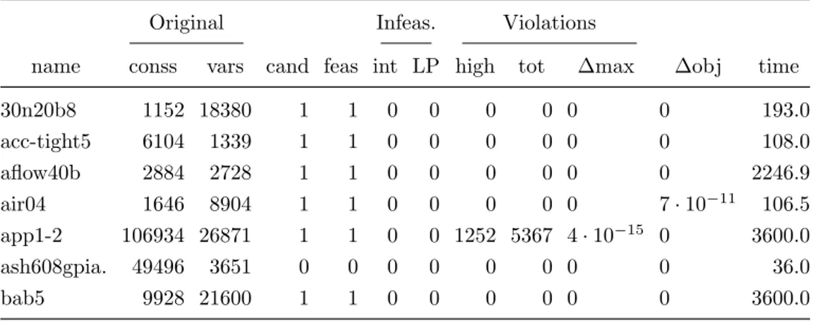
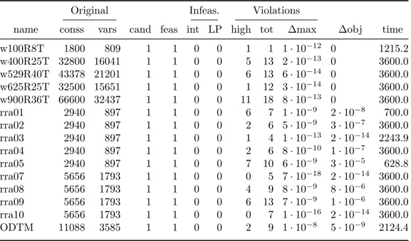
Many parameters are associated to xprim constraint handler, however we can mainly distinguish two different modes: analysis mode and enforce mode. In analysis mode the tool is passive since it simply checks the best solution found by SCIP and store information about it. This mode is used to collect statistics about how the actual version of SCIP works using floating-point numbers, since it doesn’t influence at all its evolution. The main functionality provided is to check whether SCIP best solution is or not an exactly feasible solution. It is also possible to know whether a possible infeasibility is due to either the integer or the continuous part of the solution. Moreover, constraint violations are computed to singularly check every constraint. Since SCIP computations are performed up to a certain tolerance (10−6 by default), when feasible solutions are obtained we can expect to find out violations less than the tolerance, but in general different from zero.

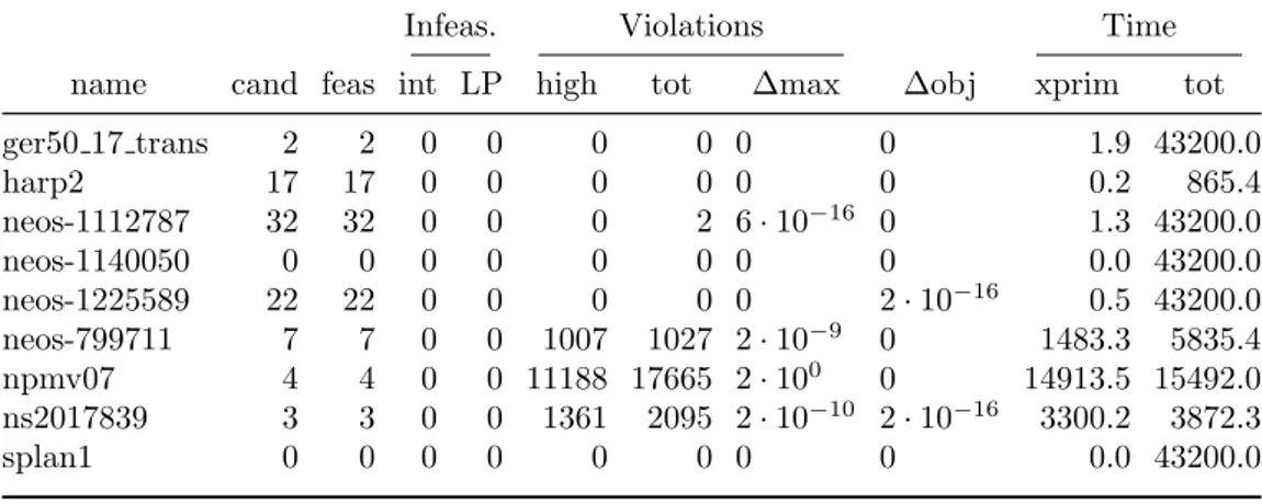
In enforce mode the tool is invoked for every feasible solution found by SCIP and it returns feedback to SCIP influencing its behavior within the tree. This mode’s target is to improve the quality of the solutions found by SCIP, discarding infeasible solutions and suggesting exact feasible solutions, when available.

The two modes share the same structure and many features. However, they clearly differ in some aspects. Since analysis mode can be considered a subset of enforce mode where only the last check is performed, in the following paragraphs the latter will be mainly considered.

3.2.2

Initialization

Every candidate solution found by SCIP solver needs to be checked by all the constraint handlers in a sequential way. Xprim constraint handler is

set to be the last invoked constraint handler, so that the input solution has already been confirmed to be feasible for all the other constraint handlers. There is a couple of explanations for that. Since the exact check is very time consuming it would be better to have the least possible number of solutions to be checked by xprim constraint handler, i.e. every solution that is infeasible for other reasons has to be discarded by previous and faster constraint handlers. Moreover, one of the purposes of xprim constraint handler is to return some statistics about the behavior of actual standard SCIP version.

Xprim constraint handler is initialized by storing an exact copy of the original problem. Constraints are obtained by means of a translation from floating-point original problem data to rational data. They are stored in the structure called SCIP ConsData, already introduced in chapter 2.3, where constraints are characterized by sides, variables and coefficients. The struc-ture also records some other useful information related to single constraints. Problem variables are characterized by bounds and objective value, i.e. the coefficient associated with the variable in the objective function. In the first tool version these values were translated from floating-point values, but in successive updates the possibility of reading rational values directly has been implemented. This improvement enhances data precision, since it removes errors due to the translation from floating-point to rationals.

The first time xprim constraint handler is invoked, an exact LP problem is set up. Originally fixed variables are marked for optimality purposes, i.e. they will not be further checked to save computation time. Constraints are divided into two subsets: integer constraints, having only integer variables, and continuous constraints, having at least one continuous variable. For optimality reasons, continuous constraints are sorted in order to have non-fixed continuous variables first. Coefficients and sides are updated by fixing values of originally fixed variables. A hash-map table is set up in order to create a mapping between original problem variables and column indexes in the exact LP.

3.2.3

Algorithm

After the set up, xprim constraint handler behavior can be summarized as follows:

3.2 Tool description 41

• solution’s integer part is rounded to the nearest integer;

• integer constraints, i.e. constraints containing only integer variables, are locally checked for feasibility;

• an exact LP is created and solved by an exact LP solver;

• exact solution and/or conflicts may be added to SCIP.

The first operation to perform every time the exact check is requested is to verify the correctness of fixings. Values of integer variables obtained by SCIP incumbent solution are rounded to the nearest integer in order to remove possible approximation errors. In general, the value of an integer variable that is supposed to be n, can be a value in the interval [n − ε, n + ε], ε < t, where t is the tolerance used by SCIP.

Integer constraints are then checked considering rounded solution. In case all constraints result to be feasible, all integer values are assumed to be correct. Consequently, left hand and right hand sides of continuous constraints are updated, leaving only continuous variables as unknowns. In the event that at least one infeasibility is observed, a conflict representing the integer part of candidate solution is added to the original problem. The new constraint is a set covering in case all involved variables are binary, otherwise is a bound disjunction. This operation allows to avoid to consider again a solution having such (infeasible) integer part as candidate.

The second step consists in solving the exact LP. QSopt ex and SoPlex can be used as exact solvers. It is important to note that the solution returned by the exact LP solver, if it exists, and the continuous part of floating-point SCIP solution are independent to each other. This follows from their different formulations, which lead, in general, to two completely different feasible solutions. This means that finding an exact LP solution does not imply that candidate solution is feasible. However, it is guaranteed that an exact feasible solution having rounded fixings as integer part and exact LP solution as continuous part exists.

Another possible approach to use in future improvements may be to solve a different exact LP aimed at minimizing the distance from the floating-point SCIP solution. With such formulation we could also estimate the magnitude of the errors on each variable.

The third and last step consists in returning feedback to SCIP. Let’s consider the case exact LP admits a feasible solution. In analysis mode it is