Ecological modelling for next generation sequencing data

Scuola di Scienze

Corso di Laurea Magistrale in Fisica

Ecological modelling for next generation

sequencing data

Relatore:

Prof. Gastone Castellani

Correlatore:

Dott. Daniel Remondini

Presentata da:

Claudia Sala

Sessione II

Le tecniche di next generation sequencing costituiscono un potente strumento per diverse applicazioni, soprattutto da quando i loro costi sono iniziati a calare e la qualit`a dei loro dati a migliorare.

Una delle applicazioni del sequencing `e certamente la metagenomica, ovvero l’analisi di microorganismi entro un dato ambiente, come per esempio quello dell’intestino. In quest’ambito il sequencing ha permesso di campionare specie batteriche a cui non si riusciva ad accedere con le tradizionali tecniche di coltura. Lo studio delle popolazioni batteriche intestinali `e molto importante in quanto queste risultano alterate come effetto ma anche causa di numerose malattie, come quelle metaboliche (obesit`a, diabete di tipo 2, etc.).

In questo lavoro siamo partiti da dati di next generation sequencing del microbiota intestinale di 5 animali (16S rRNA sequencing) (Jeraldo et al.[35]). Abbiamo ap-plicato algoritmi ottimizzati (UCLUST) per clusterizzare le sequenze generate in OTU (Operational Taxonomic Units), che corrispondono a cluster di specie bat-teriche ad un determinato livello tassonomico.

Abbiamo poi applicato la teoria ecologica a master equation sviluppata da Volkov et al.[49] per descrivere la distribuzione dell’abbondanza relativa delle specie (RSA) per i nostri campioni. La RSA `e uno strumento ormai validato per lo studio della biodiversit`a dei sistemi ecologici e mostra una transizione da un andamento a logserie ad uno a lognormale passando da piccole comunit`a locali isolate a pi`u grandi metacomunit`a costituite da pi`u comunit`a locali che possono in qualche modo interagire.

Abbiamo mostrato come le OTU di popolazioni batteriche intestinali costituis-cono un sistema ecologico che segue queste stesse regole se ottenuto usando di-verse soglie di similarit`a nella procedura di clustering.

Ci aspettiamo quindi che questo risultato possa essere sfruttato per la compren-sione della dinamica delle popolazioni batteriche e quindi di come queste variano in presenza di particolari malattie.

1 Sequencing 1

1.1 Sequencing Applications . . . 1

1.2 DNA Sequencing techniques . . . 3

1.3 Algorithms . . . 15

1.3.1 Sequence alignment . . . 15

1.3.2 Clustering methods . . . 24

1.3.3 Distances . . . 29

1.3.4 Taxonomic assignment . . . 30

2 Gut microbiota and microbioma 33 2.1 Metagenomics . . . 33

2.2 Human microbiota . . . 34

2.3 Gut microbiota and metabolic diseases . . . 34

3 The Chemical Master Equation 40 3.1 Markov processes . . . 40

3.2 The Master Equation . . . 45

3.3 Chemical Master Equation (CME) . . . 46

4 Ecological theories 50 4.1 Ecological theories purposes and perspectives . . . 50

4.2 Patterns of relative abundance - inductive approaches . . . 53

4.3 Patterns of relative abundance - deductive approaches . . . 58

4.4 Dynamical models of RSA . . . 62

4.5 Application: coral reefs . . . 68

5 Results 71 5.1 Data . . . 71

5.2 Clustering . . . 72

5.3 UCLUST tests . . . 73

A Stochastic processes - Fluctuations 94

B DNA and RNA 97

B.1 DNA and RNA as molecules . . . 97 B.2 DNA replication . . . 100 C 16S ribosomal RNA and phylogenetic analysis 103 C.1 The tree of life . . . 103 C.2 16S ribosomal RNA . . . 106

Sequencing is the mean to determine the primary structure of a biopolymer, that is for example the exact order of nucleotides in a strand of DNA.

Nowadays, sequencing techniques are assuming an increasingly important role, particularly since their costs began to decline and their methods became more simple and widespread. These next generation sequencing techniques, which de-veloped since the mid 1990s, are enabling us to gather many more times sequence data than was possible a few years ago.

Metagenomics is one of the many fields which exploit sequencing. In particular, with metagenomics we mean the collective genomes of microbes within a given environment, using indeed sequencing techniques to sequence particular strands of the genome of microorganisms. To study bacteria populations, for example, one sequences the 16S ribosomal RNA, which is a component of the 30S small subunit of prokaryotic ribosomes.

Ribosomal RNA is suitable for phylogenetic studies since it is a component of all self-replicating systems, it is readily isolated and its sequence changes but slowly with time, permitting the detection of relatedness among very distant species. Metagenomics is one of the fastest advancing fields in biology [38]. By allow-ing access to the genomes of entire communities of bacteria, virus and fungi that are otherwise inaccessible, metagenomics is extending our comprehension of the diversity, ecology, evolution and functioning of the microbial world. The con-tinuous and dynamic development of faster sequencing techniques, together with the advancement of methods and algorithms to cope with exponentially increasing amount of data generated are expanding our capacity to analyze microbial com-munities from an unlimited variety of habitats and environments.

In particular, exploiting next-generation sequencing techniques we became able to sample and study the gut microbiota biodiversity in order to understand how and why it results modified in many pathologies, such as in metabolic diseases and type 2 diabetes.

Patients affected by these pathologies, in fact, exhibit a certain degree of gut bacte-rial dysbiosis, that constitutes at the same time an effect but also a causal element of the pathology.

Many ecological theories have been proposed to understand and describe the bio-diversity of ecological communities, a problem not completely solved by now. A common element of these theories is the idea that, to study the biodiversity of a system, we shall look at the relative species abundance distribution (RSA) rather than at the static coexistence among species, since ecological populations are evolving and not static systems [34]. Furthermore, it seems that these RSA distributions vary in many ways in different ecosystems, but always show some-how similar trends.

Volkov et al. [49] suggested a simple dynamical model which well describes RSA distribution of many different ecological systems, such as for example that of the coral-reef community, starting from the chemical master equation of a birth-death process. They thus obtained a negative binomial distribution with a shape param-eter linked to immigration.

What we would like to do in this work is to exploit this dynamical model in order to describe data from gut microbiota populations, acquired through next genera-tion sequencing techniques. For this purpose, we will described the funcgenera-tioning and applications of sequencing techniques (chapter 1) and the biomedical prob-lems for which we are interested in analyzing the gut microbiota biodiversity (chapter 2). Thereafter, we will face the mathematical aspects of the chemical master equation (chapter 3), that we will exploit in the description of ecological models (chapter 4). In chapter 5 we will describe our dataset, which is a col-lection of 5 animals gut microbiota data from Jeraldo et al. [35], generated with next-generation sequencing. Then we will explain how we processed these data through specific optimized sequencing analysis algorithms, obtaining OTUs (clus-ters) which correspond to bacteria species. Finally we will show our results in the form of Preston plots, fitted with a gamma-like function, which corresponds to the continuous form of the negative binomial distribution predicted by Volkov et al. [49].

Sequencing

In this chapter, first of all, we will explain the main sequencing applications, with a particular attention to that of gut microbiota, to give an idea of the importance of this technique. Then we will explore the most common sequencing methods, from Maxam-Gilbert sequencing to next-generation sequencing. Finally, we will give an insight of the principal algorithms that permit to analyze this kind of data, through alignment, clustering, distance computation and taxonomic assignment.

In general with the term ‘sequencing’ we refer to the means to determine the pri-mary structure of a biopolymer. There are different types of sequencing (DNA se-quencing, RNA sese-quencing, protein sequencing and ChIP sequencing) and differ-ent techniques to realize it. In particular we focus on RNA/DNA sequencing, that is the process of determining the precise order of nucleotides within a strand of RNA/DNA, i.e. of the four bases (adenine, guanine, cytosine, and thymine/uracil). For insights on DNA/RNA structure and the main biological processes exploited in sequencing, we refer to appendix B.

1.1

Sequencing Applications

Sequencing vs Microarray Nowadays, sequencing techniques are assuming an increasingly important role, particularly since their costs began to decline and their methods became more simple and widespread. Thus, researchers are choos-ing sequencchoos-ing over the more common technique of microarrays, and not only for their genomic applications [22].

A DNA microarray (also commonly known as DNA chip or biochip) is a col-lection of microscopic DNA spots attached to a solid surface. These devices are used to measure the expression levels of large numbers of genes simultaneously

or to genotype multiple regions of a genome. Each DNA spot contains picomoles (1012 _{moles) of a specific DNA sequence, known as probes. These probes can}

be composed by short sections of genes or other DNA elements that are used to hybridize a cDNA or cRNA (where ‘c’ stands for ‘complementary’) sample (tar-get) under high-stringency conditions. Probes are placed in known positions of the solid surface and are fluorophore-, silver-, or chemiluminescence- labeled, so that a probe-target hybridization can be detected and quantified. Since the posi-tions and the sequences of the probes are known, we can determine the sequences present on our target, since they will hybridize with their complementary probe. The main shortcoming of microarrays is that the probe matrix can include just a limited number of sequences, thus we have to previously know the probes that we need, that is which sequences we are going to analyze. So, for example de novo sequencing is not possible.

Next-generation sequencing methods provide a valid alternative to microarrays for some applications, such as chromatin immunoprecipitation, while for others, like cytogenetics, the transition between these two techniques has barely begun. The reasons for this are that, first of all, microarrays’ longtime use as a genomics tool means many researchers are very comfortable using them, and that sample label-ing, array handling and data analysis methods are tried and true. Secondly that, despite sequencing advancements, expression arrays are still cheaper and easier when processing large numbers of samples.

Nevertheless, the fast development of sequencing in producing high throughput data at lowering costs makes us suppose that these techniques will replace mi-croarrays also in the fields in which these still rule.

Applications fields We now give a short overview of the main fields of sequenc-ing applications reported in [20].

As already mentioned, one of the main applications of sequencing, is that of de novo sequencing. The aim here is to sequence a genome not yet known.

A second field is the sequencing of the trascriptome (RNAseq) and of microRNA (a small non-coding RNA molecule of about 22 nucleotides, which functions in transcriptional and post-transcriptional regulation of gene expression). This can be considered another great tool to analyze the biological functions inside a cell, since it gives informations about the gene expression in different tissues or at dif-ferent conditions inside a certain tissue, that can be exploited in studies of RNA interference or more in general in epigenetic studies.

A third field of application is that of resequencing, where an whole already se-quenced genome needs to be resese-quenced, for example to identify any genetic deficiency such as mutations, insertions, deletions or alterations in the number of

a gene copies. This kind of analysis is very useful to understand the development of some pathologies and to find eventual clinical treatments.

Another important field of application, in which our work is included, is the se-quencing of microbiotic communities for metagenomic studies. Metagenomic sequencing allows to analyze samples directly taken from the microbiotic envi-ronment, avoiding the issue of growing bacteria artificially. In fact, as we will underline in section 2.1, traditional clonal culture techniques result biased and cannot access the vast majority of organisms within a community. In this contest the sequenced strands are those of the 16S ribosomal RNA (see appendix C), since this results highly conserved between different species of bacteria and archaea and thus can be used for phylogenetic and biodiversity studies.

One of the widest metagenomic studies, was that begun in 2003 by Craig Venter, leader of the privately funded parallel of the Human Genome Project, who has led the Global Ocean Sampling Expedition (GOS), circumnavigating the globe and collecting metagenomic samples throughout the journey. All of these sam-ples were sequenced using shotgun sequencing, in the hope that new genomes (and therefore new organisms) would be identified. The pilot project, conducted in the Sargasso Sea, found DNA from nearly 2000 different species, including 148 types of bacteria never before seen [48]. Analysis of the metagenomic data col-lected during Venter’s journey also revealed two groups of organisms, one com-posed by taxa adapted to environmental conditions of ‘feast or famine’, and a second composed by relatively fewer but more abundantly and widely distributed taxa primarily composed by plankton. Thus, this study resulted in an important turning point in ocean biodiversity knowledge, and above all it showed the great potentialities of nowadays sequencing techniques.

Finally, the last application that we are going to mention is that of Chromatin ImmunoPrecipitation-Sequencing (ChIP-seq). This technique is used to study the interaction between DNA and regulatory proteins. In fact, immunoprecipita-tion allows to identify the posiimmunoprecipita-tions on the DNA strand, on which transcripimmunoprecipita-tional factors, histones or proteins can be bound to control DNA replication. Thus, with different sequencing we can understand the influence of environmental alterations on the phenotype.

1.2

DNA Sequencing techniques

After explaining the great potentiality of sequencing, let us now give an insight of how this techniques work.

Sequencing techniques, are able to analyze just fragments of DNA. The fragment of DNA that is being read is called ‘read’, and it is composed by at most a hundred

of nucleotides. These reads then need to be processed and assembled to build the unknown sequence. We will see later the most common algorithms to analyze these reads, but for now let us describe the main techniques of DNA sequencing.

First generation DNA sequencing methods

Maxam-Gilbert sequencing Maxam-Gilbert sequencing was the first widely-adopted method for DNA sequencing, developed by Allan Maxam and Walter Gilbert in 1976-1977 and also known as the chemical degradation method. This technique is based on nucleobase-specific partial chemical modification of DNA and subsequent cleavage of the DNA backbone at sites adjacent to the modified nucleotides [41].

The first step in Maxam-Gilbert sequencing is a radioactive labeling at one 5’-end of the DNA fragment that we want to sequence. This is typically done through a kinase reaction using gamma32P ATP, where 32P is a radioactive isotope of phosphorus that decays into sulfur-32 by beta decay with a half-life of about 14 days.

The DNA fragment is then denaturated, i.e. its double strand is separated into two single strands through the breaking of the hydrogen bonds between them. After this procedure the DNA fragment is subjected to four specific chemical reactions, that generate breaks of different sizes and in different positions:

• dimethyl sulfate (DMS) plus piperdine cleaves at G; • DMS plus piperdine and formic acid cleaves at A or G; • hydrazine plus piperdine cleavs at C or T;

• hydrazine in a saline solution (NaCl) plus piperdine cleaves at C.

As shown in figure 1.1, reaction products are then electrophoresed on a polyacry-lamide denaturing gel for size separation. To visualize the fragments, the gel is exposed to an X-ray film for autoradiography, yielding a series of dark bands each showing the location of identical radiolabeled DNA molecules. The sequence can be deduced from the presence or the absence of certain fragments.

Figure 1.1: An example Maxam-Gilbert sequencing reaction from [6]. In level 1 there will be the shortest sequences and in level 7 the longest.

Sanger sequencing Sanger sequencing, also called chain-terminator sequenc-ing, has been developed by Fredrick Sanger and colleagues in 1977 and was the most widley-used method for about 25 years.

Similarly to the Maxam-Gilbert method, the DNA sample is subjected to four separate sequencing reactions. Each reaction contains the DNA polymerase, plus three of the four standard deoxynucleotides, that are the DNA nucleosides triphos-phate (dATP, dGTP, dCTP and dTTP) required for the DNA extension and only one of the four dideoxynucleotides (ddATP, ddGTP, ddCTP, or ddTTP), which are modified nucleotides that terminate the DNA strand elongation, since they lack the 3’-OH group required for the formation of the phosphodiester with the following nucleotide. When the specific ddNTP included in the reaction is incorporated in the DNA strand, the polymerase ceases the extension of DNA and we obtain DNA

fragments that terminate with a specific nucleotide. The resulting DNA fragments are then denatured and separated by size using gel electrophoresis, like in the Maxam Gilbert method. To visualize the DNA bands automatically, the ddNTPs are also radioactively or fluorescently labeled, so that the DNA bands can be vi-sualized by autoradiography or UV light and the DNA sequence can be directly read off the X-ray film or gel image [5].

The greatest limitations of Maxam - Gilbert and Sanger sequencing methods are that they are quite expensive and that they can be used just for fairly short strands (100 to 1000 basepairs). However, some improvements have been developed in order to allow the sequencing of longer strands.

Longer strands sequencing For longer targets such as chromosomes, common approaches consist of cutting (with restriction enzymes) or shearing (with me-chanical forces) large DNA fragments into shorter DNA fragments. The frag-mented DNA may then be cloned into a DNA vector and amplified in a bacterial host such as Escherichia coli. Amplification is required to have more copies of the same DNA fragment, in order to have more robust statistical informations. Short DNA fragments purified from individual bacterial colonies are individu-ally sequenced and assembled electronicindividu-ally into one long, contiguous sequence. There are two main methods used for this purpose: primer walking and shotgun sequencing.

Primer walking starts from the beginning of the DNA target, using the first 20 bases as primers for a PCR (polymerase chain reaction), that is a technique of DNA amplification, amplifying about 1000 bases and then sequencing them using the chain termination method. Then the method ‘walks’ on the DNA strand and uses the last 20 bases of the previous, now known, sequence as primers, and so on.

In shotgun sequencing, instead, DNA is broken up randomly into numerous small segments, which are sequenced using the chain termination method to obtain reads. Multiple overlapping reads for the target DNA are obtained by performing several rounds of this fragmentation and sequencing. Computer programs then use the overlapping ends of different reads to assemble them into a continuous sequence.

Next-generation DNA sequencing methods

The high demand for low-cost sequencing has driven the development of high-throughput sequencing (or next-generation sequencing) technologies that paral-lelize the sequencing process, producing thousands or millions of sequences con-currently. Nowadays, these new methods can analyze up to 600 billions of bases (GB) in a ten days cycle, versus the one million of the first generation methods, and this of course coincide with a lowering in the costs. We can give an idea of the magnitudes we deal with considering that the HIV virus genome is 3.4 kB, the E. coli bacteria genome is 4.6 MB, and the human one is 3.2 GB [20]

The main shortcoming of these new technologies is the small length of the reads, that generates errors during the assembly phase, that should be considered in fur-ther analysis.

Let us describe three of the main next-generation sequencing techniques: 454 py-rosequencing, Illumina (Solexa) sequencing and SOLiD sequencing.

454 pyrosequencing Pyrosequencing is a method of DNA sequencing based on the ‘sequencing by synthesis’ principle; it was the first next-generation method available on the market (produced by 454 Life Sciences since 2005 and now owned by Roche Diagnostics). It differs from Sanger sequencing, in that it re-lies on the detection of pyrophosphate released by nucleotide incorporation, rather than chain termination with dideoxynucleotides.

‘Sequencing by synthesis’ involves taking a single strand of the DNA sample that one wants to sequence and then synthesizing its complementary strand enzymat-ically. The pyrosequencing method is based on detecting the activity of DNA polymerase with another chemiluminescent enzyme. The template DNA is im-mobilized, and solutions of A, C, G, and T nucleotides are sequentially added and removed from the reaction, so that we can detect which base was actually added by the DNA polymerase at each step. Light is produced only when the nucleotide solution complements the first unpaired base of the template. The sequence of so-lutions which produce chemiluminescent signals allows the determination of the sequence of the template.

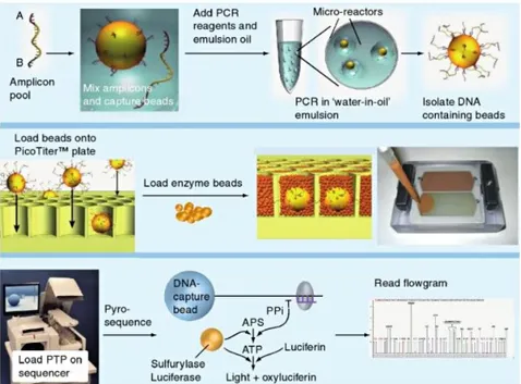
A parallelized version of pyrosequencing was developed by 454 Life Sciences [17], see fig.1.2. 454 Sequencing uses a large-scale parallel pyrosequencing sys-tem capable of sequencing roughly 400-600 megabases of DNA per 10-hour run.

In 454 pyrosequencing, DNA samples are first fractionated into smaller fragments (300-800 base pairs) and polished (made blunt at each end). Short adaptors, that are short, chemically synthesized, double stranded DNA molecules, are then lig-ated onto the ends of the fragments. These adaptors provide priming sequences for

Figure 1.2: 454 Life Sciences Sequencing Technology. Pooled amplicons are clonally amplified in droplet emulsions. Isolated DNA-carrying beads are loaded into individual wells on a PicoTiter plate and surrounded by enzyme beads. Nu-cleotides are flowed one at a time over the plate and template-dependent incorpo-ration releases pyrophosphate, which is converted to light through an enzymatic process. The light signals, which are proportional to the number of incorporated nucleotides in a given flow, are represented in flowgrams that are analyzed and a nucleotide sequence is determined for each read. Figure from [31].

both amplification and sequencing of the sample fragments. One adaptor (Adap-tor B) contains a 5’-biotin tag for immobilization of the DNA fragments onto streptavidin-coated beads. Then, the non-biotinylated strand is released and used as a single-stranded template DNA (sstDNA).

Let us observe that there should be a great number of beads (around one million), so that each bead will carry just a single sstDNA molecule. The beads are then emulsified with the amplification reagents in a water-in-oil mixture. This leads to the formation of drops of water (containing the beads) in the oil mixture, where PCR amplification occurs. This is useful, since the amplification can be done in vitro, keeping the different fragments reactions separated. This part of the process results in bead-immobilized, clonally amplified DNA fragments.

Subsequently, the beads are placed onto a PicoTiterPlate device, that is composed of around 1.6 million wells, small enough to contain just one bead (∼ 28µm of

di-ameter). The device is centrifuged to deposit the beads into the wells and the DNA polymerase is added, with also other smaller beads (containing two enzymes: sul-furylase and luciferase), which ensure that the DNA beads remain positioned in the wells during the sequencing reaction.

At this point also the sequencing reagents required by pyrosequencing are de-livered across the wells of the plate. These include ATP sulfurylase, luciferase, apyrase, the substrates adenosine 5 phosphosulfate (APS) and luciferin and the four deoxynucleoside triphosphates (dNTPs). The four dNTPs are added sequen-tially in a fixed order across the PicoTiterPlate device during a sequencing run. During the nucleotide flow, millions of copies of DNA bound to each bead are sequenced in parallel. When a nucleotide complementary to the template strand is added into a well, the polymerase extends the existing DNA strand by adding nucleotide(s). Addition of one (or more) nucleotide(s) generates a light signal that is recorded by the CCD camera in the instrument and that is proportional to the number of nucleotides. This can be explained following the biochemical reaction that occurs when the dNTP is complementary to the next nucleotide on the frag-ment. In this case, the bound between the two bases will release pyrophosphate (PPi) in stoichiometrical amounts. ATP sulfurylase quantitatively converts PPi to ATP in the presence of adenosine 5 phosphosulfate. This ATP acts as fuel to the luciferase-mediated conversion of luciferin to oxyluciferin that generates visible light in amounts that are proportional to the amount of ATP, that is proportional to the number of nucleotides bound by this dNTP type. Unincorporated nucleotides and ATP are then degraded by the apyrase enzyme, and the reaction can restart with another nucleotide.

Let us note that when the polymerase meets homopolymers, that are sequences of the same kind of nucleotide (e.g. AAAA), the contiguous bases are incorporated during the same cycle and their number can be deduced just through the intensity of the emitted light, that sometimes can be misleading.

Currently, a limitation of the method is that the lengths of individual reads of DNA sequence are in the neighborhood of 300-500 nucleotides, that is shorter than the 800-1000 obtainable with chain termination methods (e.g. Sanger sequencing). This can make the process of genome assembly more difficult, particularly for se-quences containing a large amount of repetitive DNA.

Bisides the rapid evolution of 454 pyrosequencing technology for what concern the sequencing time (it allows to sequence one million fragments in 10 hours) and costs (even if it remains the most expensive technique of next-generation sequenc-ing), this progresses have not been accompanied by a reassessment of the quality and accuracy of the sequences obtained. The mean error rate for this technology is in fact of 1.07% [33]. More importantly, this error rate is not randomly distributed; it occasionally rose to more than 50% in certain positions, and its distribution was linked to several experimental variables like the presence of homopolymers, the

position in the sequence, the size of the sequence and its spatial localization in PicoTiter plates.

Illumina (Solexa) sequencing Illumina (Solexa) sequencing was first commer-cialized by Solexa in 2006, a company later acquired by Illumina. This sequencing method is based on the reversible chain termination method described previously, and its general functioning can be subdivided in three phases: library generation, cluster preparation and sequencing.

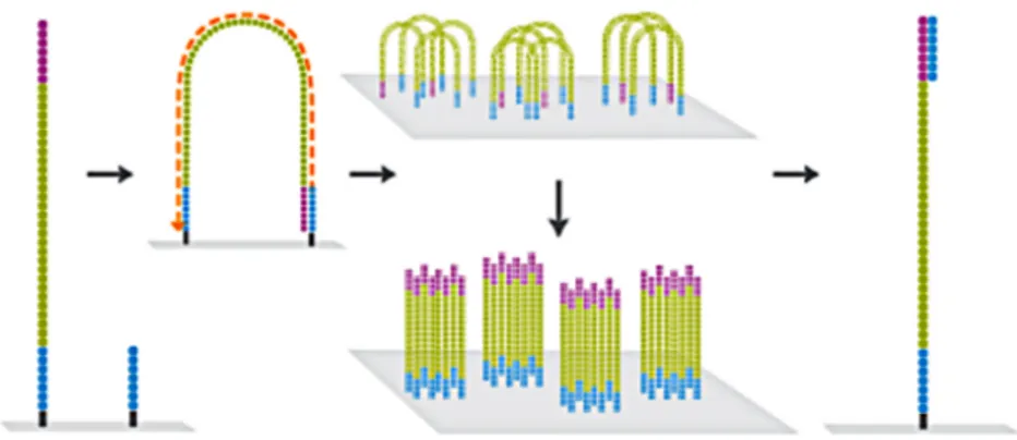
During the first phase, DNA is fragmented and oligo-adaptors are added at each fragment sides for the next amplification process. Amplification occurs on flow-cell, that is a plate on which DNA molecules are attached and on which two dif-ferent types of oligonucleotides are present. DNA fragments ends bind to these oligonucleotides, each end binding with its complementary nucleotide, so that a bridge structure is created, as shown in figure 1.3.

Figure 1.3: DNA ligated with adaptors is attached to the flow-cell; bridge am-plification is performed; clusters are generated; the sequencing primers are syn-thetizes. Figure from [8].

At this point DNA polymerase synthesizes the complementary strands of our frag-ments, that are then denaturated. The hydrogen bonds are broken and we obtain again two separated strand, doubled compared to the beginning. The process is repeated to obtain a cluster of thousands of fragments, that however contain both the original strand and the complementary one. Thus, it is necessary to remove the antisense strands, before sequencing the samples.

In the last step, primers of the fragments of each cluster are synthesized. These primers are those sequences that start the sequencing reaction. So, sequencing can

be done on millions of clusters in parallel.

Figure 1.4: The first base is extended, read and deblocked; the above step is repeated on the whole strand; the fluorescent signals are read. Figure from [8].

Each step of the sequencing process involves a DNA polymerase and the four modified dNTP, which contain also a fluorescent marker and a reversible termina-tor. Markers of the four nucleotides react in different manner when subjected to a laser wave and this allows the identification of the sequenced base (see fig.1.4). After each incorporation, a laser excites the fluorescent marker generating a light emission that allows the identification of the base. Then the terminator and the fluorescent label are removed, so that the next base can be sequenced.

With a single cycle, Illumina sequencer can read up to 6 billion reads in few days, with a number of bases ranging from 50 to 200, that means a total of almost 1000 GBases.

SOLiD sequencing Applied Biosystems’ (now a Life Technologies brand) SOLiD technology employs sequencing by ligation. Like in 454 pyrosequencing, DNA fragments are bound to adaptors in order to immobilize them onto beads and to amplify them through emPCR. After denaturation, beads are placed on a glass support; the difference between this support and the PicoTiter plate is that in SOLiD there are no wells, thus the only limitation on the number of beads is due to their diameter, that now is much smaller than for the 454 technologies (< 1µm). In SOLiD, sequencing by synthesis is driven by DNA ligase, rather than polymerase, that is an enzyme that facilitates the joining of DNA strands together by catalyzing the formation of a phosphodiester bond, hence the acronym SOLiD (Sequencing by Oligonucleotide Ligation and Detection).

Each sequencing cycle needs a bead, a degenerate primer (which can bind all the four bases), a ligase and four dNTP 8-mer probe, which are eight bases in length with a free hydroxyl group at the 3’ end, with a fluorescent dye at the 5’ end and with a cleavage site between the fifth and sixth nucleotide. The first two bases (starting at the 3’ end) are complementary to the nucleotides being sequenced, while bases 3 through 5 are degenerate and able to pair with any nucleotides on the template sequence.

First of all the primer hybridizes with the adaptor sequence, then the ligase allows the bound of a probe, followed by fluorescent emission from the dye; finally, the last three bases (6-7-8) of the 8-mer bound are removed together with the dye, to allow the analysis of subsequent bases.

Each couple of bases is associated with a particular color to allow the identifica-tion; however the labeling is not univocal, since we have 4 colors and 16 possible couples of bases. So, we can wonder why associating a color to each couple rather than to each base. Actually, the method used here is more convenient since using a 1-1 corrispondence is more probable to generate sequencing errors, while this method can help in avoiding them (see fig.1.5). Let us note that, since in each cy-cle we will sequence 2 nucy-cleotides every 5, we will have to repeat the sequencing cycle five times to univocally determine each base (see fig.1.6).

During this process, just few 8-mers can be bound together (7, or at most 10), and this lead to very short reads (35-50 bases), but at the same time this procedure allows a minimization of the errors during each read scanning.

Figure 1.5: How SOLiD responds to single mutations, measurement errors, dele-tions and inserdele-tions. Figure from [9].

Figure 1.6: Color output of the template TAGACA. Because of the end-labeling, all sequences start with a T, therefore since the first signal output is blue, the first base-pair of the sequence must be a T, since the only blue probe that begins with an A (complementary to the T) is the AA probe. The machine uses the same logic to compute the entire strand. Figure from [39].

Specifications summary

Figure 1.7: Specifications of different sequencing techniques. Figure from [20].

Computational requirements

The high performances of these next-generation techniques led to the need of also high computational ability for what concern both data storage and elaboration [20].

We have to consider, in fact, that for each sequenced base, we can have up to 16 byte (but also more), and that a Illumina or SOLiD run can need some Tbyte of memory, neglecting eventual backup and redundances. To give an idea of the amount of data produced by next-generation sequencing platform, we can refer to the 9 petabyte (18 · 1050_{byte) generated in 2010 by the Sanger Insitute alone, that}

is one of the biggest sequencing center in the world.

Furthermore, these big amount of data need to be processed and analyzed: reads need to be assembled and/or aligned. Thus, besides the storage memory, also high-performances CPU and algorithms are needed.

1.3

Algorithms

Usually, sequencing data analysis includes the following processing procedures: alignment, distances computations, clustering and taxonomic assignment. Let us now describe the principal optimized algorithms to compute these elaborations. We will exploit these algorithms through QIIME (Quantitative Insights Into Mi-crobial Ecology) [12], that is an open source software package for comparison and analysis of microbial communities, primarily based on high-throughput sequenc-ing data generated on a variety of platforms, but also supportsequenc-ing analysis of other types of data (such as shotgun metagenomic data). QIIME takes users from their raw sequencing output through initial analyses such as OTU picking, taxonomic assignment, and construction of phylogenetic trees from representative sequences of OTUs, and through downstream statistical analysis, visualization, and produc-tion of publicaproduc-tion-quality graphics.

1.3.1

Sequence alignment

Computational algorithms to sequence alignment generally fall into two cate-gories: global alignments and local alignments.

Calculating a global alignment is a form of global optimization that ‘forces’ the alignment to span the entire length of all query sequences. These methods are more useful when the sequences in the query set are similar and of roughly equal size.

By contrast, local alignments identify regions of similarity within long sequences that are often widely divergent overall. Thus, these methods are more useful for dissimilar sequences that are suspected to contain regions of similarity or similar sequence motifs within their larger sequence context. Local alignments are often preferable, but can be more difficult to calculate because of the additional chal-lenge of identifying the regions of similarity. One motivation for local alignment is the difficulty of obtaining correct alignments in regions of low similarity between distantly related biological sequences, because mutations have added too much ‘noise’ over evolutionary time to allow for a meaningful comparison of those re-gions. Local alignment avoids such regions altogether and focuses on those with an evolutionary conserved signal of similarity.

There exist also hybrid methods, which attempt to find the best possible alignment that includes the start and end of one or the other sequence. This can be especially useful when the downstream part of one sequence overlaps with the upstream part of the other sequence. In this case, neither global nor local alignment would en-tirely work.

align-ment problem. These include slow but formally correct methods like dynamic pro-gramming, but also include efficient, heuristic algorithms or probabilistic meth-ods designed for large-scale database search, that do not guarantee to find best matches.

Smith-Waterman Early alignment programs, such as the Smith-Waterman al-gorithm and the Needleman-Wunsch, which is a variation of the first one, used dynamic programming algorithms, that is methods based on the idea that to solve complex problems one can break them down into simpler subproblems. Often when using a more naive method, many of the subproblems are generated and solved many times. The dynamic programming approach seeks to solve each sub-problem only once, thus reducing the number of computations: once the solution to a given subproblem has been computed, it is stored: the next time the same so-lution is needed, it is simply looked up. This approach is especially useful when the number of repeating subproblems grows exponentially as a function of the size of the input.

Dynamic programming algorithms are used for optimization (for example, finding the shortest path between two points, or the fastest way to multiply many matri-ces). A dynamic programming algorithm will examine all possible ways to solve the problem and will pick the best solution. Therefore, we can roughly think of dynamic programming as an intelligent, brute-force method that enables us to go through all possible solutions to pick the best one. If the scope of the problem is such that going through all possible solutions is possible and fast enough, dy-namic programming guarantees finding the optimal solution.

The Smith-Waterman algorithm is a dynamic programming method which per-forms local sequence alignment with the guarantee of finding the optimal align-ment [15].

The algorithm first builds a matrix H as follows:

H(i, 0) = 0; for 0 ≤ i ≤ m

H(0, j) = 0; for 0 ≤ j ≤ n (1.1) Then, if ai = bj then w(ai, bj) = w(match) or if ai 6= bj then w(ai, bj) =

w(mismatch), thus for 1 ≤ i ≤ m, 1 ≤ j ≤ n, we have

H(i, j) = max        0

H(i − 1, j − 1) + w(ai, bj) Match/Mismatch

H(i − 1, j) + w(ai, −) Deletion

H(i, j − 1) + w(−, bj) Insertion        . (1.2) where:

• a, b = strings that we want to align; • m = length(a);

• n = length(b).

Let us now show an example from [15]. Sequence 1 = ACACACTA Sequence 2 = AGCACACA w(match) = +2 w(a, −) = w(−, b) = w(mismatch) = −1 H =                 − A C A C A C T A − 0 0 0 0 0 0 0 0 0 A 0 2 1 2 1 2 1 0 2 G 0 1 1 1 1 1 1 0 1 C 0 0 3 2 3 2 3 2 1 A 0 2 2 5 4 5 4 3 4 C 0 1 4 4 7 6 7 6 5 A 0 2 3 6 6 9 8 7 8 C 0 1 4 5 8 8 11 10 9 A 0 2 3 6 7 10 10 10 12                 (1.3) T =                 − A C A C A C T A − 0 0 0 0 0 0 0 0 0 A 0 - ← - ← - ← ← -G 0 ↑ - ↑ - ↑ - - ↑ C 0 ↑ - - - ← - ← ← A 0 - ↑ - ← - ← ← -C 0 ↑ - ↑ - ← - ← ← A 0 - ↑ - ↑ - ← ← -C 0 ↑ - ↑ - ↑ - ← ← A 0 - ↑ - ↑ - ↑ -                (1.4)

To obtain the optimum local alignment, we start with the highest value in the ma-trix (i, j). Then, we go backwards to one of positions (i − 1, j), (i, j − 1), and (i−1, j −1) depending on the direction of movement used to construct the matrix. We keep the process until we reach a matrix cell with zero value.

In the example, the highest value corresponds to the cell in position (8, 8). The walk back corresponds to (8, 8), (7, 7), (7, 6), (6, 5), (5, 4), (4, 3), (3, 2), (2, 1), (1, 1), and (0, 0).

Once we’ve finished, we reconstruct the alignment as follows: starting with the last value, we reach (i, j) using the previously calculated path. A diagonal jump

implies there is an alignment (either a match or a mismatch). A top-down jump implies there is a deletion. A left-right jump implies there is an insertion.

For our example, we get: Sequence 1 = A-CACACTA Sequence 2 = AGCACAC-A

The Smith-Waterman algorithm is fairly demanding of time: to align two se-quences of lengths m and n, O(mn) time is required. Other algorithms such as BLAST, that we are now going to describe, reduce the amount of time required by identifying conserved regions using rapid lookup strategies, at the cost of ex-actness.

BLAST and FASTA BLAST (Basic Local Alignment Search Tool) and FASTA (FAST All) are heuristic algorithms, and as such they are designed for solving a problem more quickly when classic dynamic methods are too slow, or for finding an approximate solution when classic methods fail to find any exact solution. By trading optimality, completeness, accuracy, and/or precision for speed, a heuristic method can quickly produce a solution that is good enough for solving the prob-lem at hand, as opposed to finding all exact solutions in a prohibitively long time. Thus heuristic algorithms are more practical for the analysis of the huge genome databases currently available.

BLAST is more time-efficient than FASTA by searching only for the more sig-nificant patterns in the sequences, yet with comparative sensitivity; thus we will focus mostly on BLAST.

To run, BLAST requires a query sequence to search for, and a sequence to search against (also called the target sequence) or a sequence database containing many target sequences. BLAST will find sub-sequences in the database which are sim-ilar to subsequences in the query. In typical usage, the query sequence is much smaller than the database, e.g., the query may be one thousand nucleotides while the database is several billion nucleotides.

The main idea of BLAST is that there are often high-scoring segment pairs (HSP) contained in a statistically significant alignment. BLAST searches for high scor-ing sequence alignments between the query sequence and sequences in the database using a heuristic approach that approximates the Smith-Waterman algorithm, that, as we already observed, is too slow for searching large genomic databases such as GenBank.

Let us report how BLAST basically works, as described in [18].

1. Remove low-complexity regions or sequence repeats in the query sequence, where ‘low-complexity’ region means a region of a sequence composed of

few kinds of elements. These regions might give high scores that confuse the program to find the actual significant sequences in the database, so they should be filtered out. The regions will be marked with an X (protein se-quences) or N (nucleic acid sese-quences) and then be ignored by the BLAST program.

2. Make a list of all the k-letter words inside the query sequence, where k usu-ally is 3 for proteins and 11 for nucleotides.

3. List the possible matching words. This step is one of the main differences between BLAST and FASTA. FASTA cares about all of the common words in the database and query sequences that are listed in step 2; however, BLAST only cares about the high-scoring words. The scores are created by comparing the words in the step 2 list with all the k-letter words and giving a score according to how many matching and non-matching words are present.

4. Organize the remaining high-scoring words into an efficient search tree. This allows the program to rapidly compare the high-scoring words to the database sequences.

5. Repeat step 3 to 4 for each k-letter word in the query sequence.

6. The BLAST program scans the database sequences for the high-scoring word of each position. If an exact match is found, this match is used to seed a possible un-gapped alignment between the query and database se-quences.

7. Extend the exact matches to high-scoring segment pair (HSP). The original version of BLAST stretches a longer alignment between the query and the database sequence in the left and right directions, from the position where the exact match occurred. The extension does not stop until the accumulated total score of the HSP begins to decrease. A simplified example is presented in fig.1.8.

Figure 1.8: The process to extend the exact match. Figure from [18].

To save more time, a newer version of BLAST, called BLAST2, adopts a lower neighborhood word score threshold to maintain the same level of sen-sitivity for detecting sequence similarity. Therefore, the possible matching words list in step 3 becomes longer. Next, the exact matched regions, within distance A from each other on the same diagonal in fig.1.9, will be joined as a longer new region.

Finally, the new regions are then extended by the same method as in the original version of BLAST, and the HSPs’ scores of the extended regions are then created as before.

Figure 1.9: The positions of the exact matches. Figure from [18].

8. List all of the HSPs in the database whose score is higher then an empirically determined cutoff score S. By examining the distribution of the alignment scores modeled by comparing random sequences, a cutoff score S can be determined such that its value is large enough to guarantee the significance of the remaining HSPs.

9. Evaluate the significance of the HSP score (E-value), that is the number of times a random database sequence would give a score higher than S by chance.

10. Make two or more HSP regions into a longer alignment. Sometimes, we find two or more HSP regions in one database sequence that can be made into a longer alignment. This provides additional evidence of the relation between the query and database sequence. There are two methods, the Pois-son method and the sum-of-scores method, to compare the significance of the newly combined HSP regions. Suppose that there are two combined HSP regions with the pairs of scores (65, 40) and (52, 45), respectively. The Poisson method gives more significance to the set with the maximal lower score (45 > 40). However, the sum-of-scores method prefers the first set, because 65 + 40 (105) is greater than 52 + 45 (97). The original BLAST uses the Poisson method; BLAST2 uses the sum-of scores method.

11. Show the gapped Smith-Waterman local alignments of the query and each of the matched database sequences. The original BLAST only generates un-gapped alignments including the initially found HSPs individually, even when there is more than one HSP found in one database sequence. BLAST2 produces a single alignment with gaps that can include all of the initially-found HSP regions. Note that the computation of the score and its corre-sponding E score is involved with the adequate gap penalties.

12. Report every match whose expect score is lower than a threshold parameter E.

Clustal W There are three main steps [42]:

1. all pairs of sequences are aligned separately in order to calculate a distance matrix giving the divergence of each pair of sequences;

2. a guide tree (or a user-defined tree) is calculated from the distance matrix;

3. the sequences are progressively pairwise aligned according to the branching order in the guide tree. Thus, first are considered the nearest sequences and then the farther. At each stage, gaps can be introduced.

In the original CLUSTAL programs, the pairwise distances are calculated giving a score to the number of matches and a penalty for each gap. The latest versions allow to choose between this method and the slower but more accurate scores from full dynamic programming alignments using two gap penalties, which differ if there is an opening gap or an extending one. These scores are calculated as the number of identities in the best alignment divided by the number of residues compared (gaps excluded). Both of these scores are initially calculated as per cent identity scores and are converted to distances by dividing per 100 and subtracting from 1.0 to give the number of differences per site.

The main advantage of CLUSTALW on previous methods is that it gives a better quality without affecting the costs.

MUSCLE MUSCLE [28] is often used as a replacement for Clustal, since it typically (but not always) gives better sequence alignments and is significantly faster than Clustal, especially for larger alignments. However, it remains quite slow compared to other methods like NAST [4].

The main steps of MUSCLE are the same of CLUSTAL: distance matrix com-putation, guide tree comcom-putation, pairwise alignment following the guide tree. MUSCLE exploits the Kimura distance, which is a more accurate measurement even if it requires a previous alignment, and the subdivision of the tree in subtrees in which the profile of multiple alignment is computed so that, with a re-alignment of these profiles one can try to find an eventual better score.

UCLUST UCLUST [2] creates multiple alignments of clusters. Thus, it re-quires a first step of clustering, then a conversion to .fasta and finally the insertion of additional gaps. We will explain in more detail the clustering step in subsection 1.3.2.

NAST In NAST [27], an unaligned sequence is termed the ‘candidate’ and is matched to templates by comparison of 7-mers in common.

At first, a BLAST pairwise alignment is performed between the candidate and the template. As a result of the pairwise alignment performed by BLAST, new alignment gaps (hyphens) are introduced between the bases of the template when-ever the candidate contains additional internal bases (insertions) compared with the template (fig.1.10 A, B). Any pairwise alignment algorithm must do this to compensate for nucleotides not shared by both sequences. This expansion, when intercalated with the original template spacing, results in candidates occupying more columns (characters) than the original template format (fig.1.10 C). Since

a consistent column count may be an option chosen by the user, the candidate-template alignment is compressed back to the initial number of characters with NAST. After insertion bases are identified (fig.1.10 C), a bidirectional search for the nearest alignment space (hyphen) relative to the insertion results in character deletion of the proximal place holders. Ultimately, local misalignments, spanning from the insertion base to the deleted alignment space, are permitted to preserve the global multiple sequence alignment format.

Figure 1.10: Example of NAST compression of a BLAST pairwise alignment using a 38 character aligned template. Figure from [27].

Others Other common alignment methods that we just mention are: MAFFT, which compute a multiple sequence alignment based on the fast Fourier transform (FFT); T-Coffee, which uses a progressive approach; INFERNAL, which tries to be more accurate and more able to detect remote homologous modeling sequences structure; mothur, through which one can do three different kinds of alignments: blastn (local), gotoh (global), and needleman (global).

1.3.2

Clustering methods

Besides alignment, another important step in sequence analysis is that of cluster-ing sequences into OTUs (Operational Taxonomic Units). An OTU is a cluster of similar sequences, within a user defined threshold.

Clustering into OTU will be exploited in 16S rRNA sequencing analysis. In fact, for how these sequences are (see appendix C), a cluster of similar elements will correspond to bacteria in the same taxon at a particular taxonomic level.

BLAST BLAST first aligns the sequences using the homonymous method and then computes a single-linkage clustering [19], that is one of several methods of agglomerative hierarchical clustering. In the beginning of the process, each ele-ment is in a cluster of its own. The clusters are then sequentially combined into larger clusters, until all elements end up being in the same cluster. At each step, the two clusters separated by the shortest distance are combined. The definition of ‘shortest distance’ is what differentiates between the different agglomerative clustering methods. In single-linkage clustering, the link between two clusters is made by a single element pair, namely those two elements (one in each cluster) that are closest to each other. The shortest of these links that remains at any step causes the fusion of the two clusters whose elements are involved. The method is also known as nearest neighbor clustering.

However, this method has different drawbacks. First of all, with the single-linkage clustering there will be the so-called chaining phenomenon, which refers to the gradual growth of a cluster as one element at a time gets added to it. This may lead to impractically heterogeneous clusters and difficulties in defining classes that could usefully subdivide the data. Moreover, BLAST is not really efficient in clustering divergent sequences, it can yield one-sequence clusters and it has a high dependency on the parameters choice (similarity threshold, identity percent-age, alignment length). Finally, this algorithm is quite slower than other methods since it compares each sequence with all the others, a fact that makes it not suit-able for large databases.

CD-HIT CD-HIT [1] has the main advantage of having ultra-fast speed. It can be hundreds of times faster than other clustering programs, like BLAST. There-fore it can handle very large databases. The main reason for this is that, unlike BLAST, which compute the all vs all similarities, CD-HIT can avoid many pair-wise sequence alignments exploiting a short word filter.

are first sorted in order of decreasing length. The longest one becomes the rep-resentative of the first cluster. Then, each remaining sequence is compared to the representatives of existing clusters. If the similarity with any representative is above a given threshold, it is grouped into that cluster. Otherwise, a new cluster is defined with that sequence as the representative.

Here is how the short word filter works. Two strings with a certain sequence iden-tity must have at least a specific number of identical words. For example, for two sequences to have 85% identity over a 100-residue window they have to have at least 70 identical 2-letter words, 55 identical 3-letter words, and 25 identical 5-letter words. By understanding the short word requirement, CD-HIT skips most pairwise alignments because it knows that the similarity of two sequences is be-low certain threshold by simple word counting.

A limitation of short word filter is that it can not be used below certain cluster-ing thresholds, where the number of identical k-letter words could be zero (see fig.1.11).

Figure 1.11: Short word filtering is limited to certain clustering thresholds. Evenly distributed mismatches are shown in alignments with 80%, 75%, 66.67% and 50% sequence identities. The number of common 5-letter words in (a), 4-letter words in (b), 3-4-letter words in (c), and 2-4-letter words in (d) can be zero. Figure from [1].

Another drawback of the algorithm is that it can happen that a sequence is more similar to a certain sequence but is put in the cluster of another one because it is compared first with this last one. Finally, two additional limitations are that CD-HIT does not give a hierarchical relation among clusters, and that it can yield one-sequence clusters.

Mothur There are three main steps in mothur [10]: • aligns sequences;

• clustering.

For the clustering step mothur can use three different methods:

• nearest neighbor: each of the sequences within an OTU are at most X% distant from the most similar sequence in the OTU;

• furthest neighbor: all of the sequences within an OTU are at most X% dis-tant from all of the other sequences within the OTU;

• average neighbor: this method is a middle ground between the other two algorithms.

Prefix/Suffix These methods [Qiime team, unpublished] collapse sequences which are identical in their first and/or last bases (i.e., their prefix and/or suffix). The pre-fix and sufpre-fix lengths are provided by the user and default to 50 each.

Trie Trie [Qiime team, unpublished] collapses identical sequences and sequences which are subsequences of other sequences.

USEARCH USEARCH [29] creates ‘seeds’ of sequences which generate clus-ters based on percent identity, filtering low abundance clusclus-ters. USEARCH can perform de novo or reference based clustering.

UCLUST UCLUST [2] is a method based on USEARCH. Its main advantages over previous methods are that it is faster, it uses less memory, it has an higher sensitivity and it is able to classify bigger datasets. We will describe this algorithm in more detail, since it is the one that we will use in our analysis.

The core step in the UCLUST algorithm is searching a database stored in mem-ory. UCLUST performs de novo clustering by starting with an empty database in memory. Query sequences are processed in input order. If a match is found to a database sequence, then the query is assigned to its cluster (first figure below), otherwise the query becomes the seed of a new cluster (second figure below). Of course the first sequence in the input file will be the first seed of the database.

Figure 1.12: Schematic representation of the working of UCLUST if the query sequence matches a seed. Figure form [2].

Figure 1.13: Schematic representation of the working of UCLUST if the query sequence does not match any seed. Figure form [2].

In this procedure, we say that a query sequence matches a database sequence if their similarity is high enough. Similarity is calculated from a global alignment, i.e. an alignment that includes all letters from both sequences. This differs from BLAST and most other database search programs, which search for local matches. The minimum identity is set in QIIME by the -s option, e.g. -s 0.97 means that

the global alignment must have at least 97% similarity. Similarity is computed as the number of matching (identical) letters divided by the length of the shortest sequence.

Let us observe that only seeds need to be stored in memory (because other cluster members do not affect how new query sequences are processed). This is an advan-tage for large datasets because the amount of memory needed and the number of sequences to search are reduced. However, this design may not be ideal in some scenarios because it allows non-seed sequences in the same cluster to fall below the identity threshold.

By default UCLUST stops searching when it finds a match. Usually UCLUST finds the best match first, but this is not guaranteed. If it is important to find the best possible match (i.e., the database sequence with highest similarity), then you can increase the --max accepts option, even if in QIIME, the default value is 20, that is already increased compared to the default UCLUST value, that is 1. UCLUST also stops searching if it fails to find a match. By default, it gives up af-ter 8 failed attempts. Database sequences are tested in an order that correlates well (but not exactly) with decreasing similarity. This means that the more sequences get tested, the less likely it is that a match will be found later, so giving up early does not miss a potential hit very often. You can set the maximum number to try using the --max rejects option, that in QIIME is 500 by default. With very high and very low similarity thresholds, increasing maxrejects can significantly improve sensitivity. Here, a rule of thumb is that low similarity is below 60% for amino acid sequences or 80% for nucleotides, high similarity is 98% or more. By default, the target sequences are rejected if they have too few unique words in common with the query sequence. The threshold is estimated using heuristics. This improves speed, but may also reduce sensitivity. In QIIME there is the pos-sibility to change the length of these words and to disable this option with the --word length command.

An ‘optimal’ variant of the algorithm can be used specifying -A (--optimal uclust), which is equivalent to setting --max accepts and --max rejects to 0 and to disable the rejection due to few words in common. This guarantees that every seed will be aligned to the query, and that every sequence will therefore be assigned to the highest-similarity seed that passes the similarity threshold (t). All pairs of seeds are guaranteed to have similarity < t. The number of seeds is guaranteed to be the minimum that can be discovered by greedy list removal, though it is possible that the number of clusters could be reduced by using a different set of seeds. An ‘exact’ variant of the algorithm is selected by -E (--exact uclust), which is equivalent to setting --max accepts to 1, --max rejects to 0 and to disable the re-jection due to few words in common. This guarantees that a match will be found if one exists, but not that the best match will be found. The exact and optimal vari-ants are guaranteed to find the minimum possible of clusters and both guarantee

that all pairs of seeds have identities < t. Exact clustering will be faster, but may have lower average similarity of non-seeds to seeds.

UCLUST supports a rich set of gap penalty options, even if in QIIME there is not a direct way to change them, probably because the default settings are consid-ered optimized. By default, terminal gaps are penalized much less than interior gaps, which is typically appropriate when fragments are aligned to full-length se-quences.

By default, UCLUST seeks nucleotide matches in the same orientation (i.e., plus strand only). You can enable both plus and minus strand matching by using -z (--enable rev strand match). This command approximately doubles memory use but results in only small increases in execution time.

As we said at the beginning of this subsection, in UCLUST query sequences are processed in input order. This means that if a query was similar to more than a seed within the threshold, it will be put in the cluster of the sequence that was first in input order. Input sequences should therefore be ordered so that the most appropriate seed sequence for a cluster is likely to be found before other mem-bers. For example, ordering by decreasing length is desirable when both complete and fragmented sequences are present, in which case full-length sequences are generally preferred as seeds since a fragment may attract longer sequences that are dissimilar in terminal regions which do not align to the seed. In other cases, long sequences may make poor seeds. For example, with some high-throughput sequencing technologies longer reads tend to have higher error rates, and in such cases sorting by decreasing read quality score may give better results.

By default, UCLUST checks that input sequences are sorted by decreasing length, unless -D (--suppress presort by abundance uclust) is specified. This check can be disabled by specifying the -B (--user sort) option, which specifies that input sequences have been pre-sorted in a way that might not be decreasing length.

1.3.3

Distances

mothur For computation of the distance matrix we will use mothur’s command dist.seqs [3]. This algorithm is well optimized, since the distances are not stored in RAM, but they are printed directly to a file. Furthermore, it is possible to ignore large distances that one might not be interested in.

To run dist.seqs an alignment file must be provided in fasta format, so sequences should be aligned before computing their distances.

By default an internal gap is only penalized once, a string of gaps is counted as a single gap, terminal gaps are penalized (there is some discussion over whether to penalize them or not), all distances are calculated, and only one processor is used. You can change all these option through the corresponding commands.

The distances are computed as in the following example. SequenceA: ATGCATGCATGC

SequenceB: ACGC - - - CATCC

Here, there would be two mismatches and one gap. The length of the shorter se-quence is 10 nt, since the gap is considered as a single position. Therefore the distance would be 3/10 or 0.30.

1.3.4

Taxonomic assignment

RDP classifier For 16S rRNA taxonomic assignment, the most common algo-rithm is the RDP classifier [14].

The RDP Classifier is distributed with a pre-built database of assigned sequences, which is used by default. Each rRNA query sequence is assigned to a set of hierar-chical taxa using a naive Bayesian rRNA classifier. The classifier is trained on the known type strain 16S sequences (and a small number of other sequences repre-senting regions of bacterial diversity with few named organisms). The frequencies of all sixty-four thousand possible 8-base subsequences (words) are calculated for the training set sequences in each of the approximately 880 genera.

When a query sequence is submitted, the joint probability of observing all the words in the query can be calculated separately for each genus from the training set probability values. Using the naive Bayesian assumption, the query is most likely a member of the genera with the highest probability. In the actual analy-sis, the algorithm randomly selects only a subset of the words to include in the joint probability calculation, and the random selection and probability calculation is repeated for 100 trials. The number of times a genus is most likely out of the 100 bootstrap trials gives an estimate of the confidence in the assignment to that genus. For higher-order assignments, the algorithm sums the results for all genera under each taxon.

For each rank assignment, the Classifier automatically estimates the classification reliability using bootstrapping. Ranks where sequences could not be assigned with a bootstrap confidence estimate above the threshold are displayed under an artificial ’unclassified’ taxon. The default threshold is 80%.

For partial sequences of length shorter than 250 bps (longer than 50 bps), a boot-strap cutoff of 50% was shown to be sufficient to accurately classify sequences at the genus level, and to provide genus level assignments for higher percentage of sequences (fig.1.14) [26].

Figure 1.14: Of 7208 full-length 16S reference sequences from the human gut 6054 were classified at genus-level with 80% bootstrap support. With these full-length assignments as references the V3, V4 and V6 regions were extracted and re-classified at three different bootstrap thresholds, and compared with the full-length classification (last row). Figure form [26].

We can choose to use 50% as bootstrap cut-off since the accuracy is closest to the one with 80% cut-off, and the total number of sequences that could be assigned to genus level is closest to that obtained without any cut-off threshold imposed.

Others Other methods exploited in QIIME are the following [13].

• BLAST. Taxonomy assignments are made by searching input sequences against a BLAST database of pre-assigned reference sequences. If a satis-factory match is found, the reference assignment is given to the input se-quence. This method does not take the hierarchical structure of the taxon-omy into account, but it is very fast and flexible.

• RTAX. Taxonomy assignments are made by searching input sequences against a fasta database of pre-assigned reference sequences. All matches are col-lected which match the query within 0.5% identity of the best match. A taxonomy assignment is made to the lowest rank at which more than half of these hits agree.

• mothur. The mothur software provides a naive bayes classifier similar to the RDP Classifier. A set of training sequences and id-to-taxonomy as-signments must be provided. Unlike the RDP Classifier, sequences in the training set may be assigned at any level of the taxonomy.

In their study, Claesson et al. [26] compared different algorithms for taxonomic assignment and found out that the Greengenes and RDP-classifier produced the most accurate and stable results, especially for gut communities. Furthermore, the

RDP-classifier resulted more than 30 times faster than the Greengenes classifier. Thus, they chose the RDP classifier due to its documented accuracy and stabil-ity, straightforward usage, independence of sequence alignments, high speed, and suitability for very large datasets generated by next-generation sequencing tech-nologies, and so we will do.

Gut microbiota and microbioma

In this chapter we will provide an insight of the gut microbiota as a biomedical issue, in order to give an idea of the importance of this ecosystem and its biodiver-sity for our health, reminding how the latest sequencing techniques and ecological theories are necessary for this purpose.

2.1

Metagenomics

Classical microbiology relied largely on the culturing and analysis of microbes isolated from environmental samples. However, in the 1990s studies based on the real cell counts using microscopy techniques and 16S rRNA phylogenetic pro-filing, estimated that the currently cultivatable microorganisms represent only a small fraction (less than 1%) of the total microbes within a given habitat [38]. Thus traditional clonal culture techniques result biased and cannot access the vast majority of organisms within a community.

Metagenomics is a mean to overcome these issues by capturing and analyzing the genetic material of the entire microbial community (i.e. the metagenome), relying on the cultivation-independent extraction of total environmental DNA.

Thus metagenomics exploits sequencing techniques (see chapter 1) to answer questions such as: how many different species inhabit a particular environment, what is the genomic potential of that community (i.e. which genes, functions or pathways are present), which species are responsible for which activities, and how does the community change over time and under different environmental condi-tions [38].

In particular, in our work we are going to analyze gut microbiota data of next-generation sequencing and to model them through ecological theories to give bio-diversity informations (see chapter 4).

2.2

Human microbiota

As reported in [38], the human body is home to roughly 10 times more microbial cells than human cells. These commensal and not pathogenic microorganisms (called human microbiota) come from all three domains of life: bacteria, archaea, and eukaria, as well as viruses, and are found mostly in the gastrointestinal tract but also along the skin surface, oral and nasal cavities, and urogenital tracts. The collective genomes of all these symbiotic microorganisms (called human micro-biome) constantly interacts with the human genomes, making humans ‘superor-ganisms’ harboring these two integrated genomes. It is through their interaction with our living environment that the human health phenotype is defined; than it is this interaction that we should consider in the study of systemic diseases.

Through the diet we influence the composition of bacteria living environment and therefore of bacteria population in our gut, yielding to a change in the metabo-lites production by the microbiota, that can get into our bloodstream via a nor-mal route enterohepatic circulation or through partially impaired gut barrier and eventually influence human health. In particular changing patterns of food con-sumption has been closely linked with the dramatic increase in the incidence of obesity, diabetes, and cardiovascular diseases, linked with variations in gut mi-crobiota distribution. Furthermore gut mimi-crobiota exhibits significant changes in response to health changes, even in the early phase in which these are not yet de-tectable, like during the development of precancerous lesions in the gut. These features make gut microbiota both a biomarker for health changes and a target for nutritional/medicinal interventions in chronic diseases.

2.3

Gut microbiota and metabolic diseases

Gut microbiota - normal functioning

The human gut is composed of four main regions: the oesophagus, the stom-ach, the small intestine, and the large intestine, constituted by the caecum and the colon. Through molecular analysis of gut microorganisms sampled through biopsies or luminal content analysis, researchers have obtained an outline of gut microbial diversity.

The first results from these analyses indicated that the same bacterial phyla tend to predominate in the stomach, small intestine, caecum and large intestine. Thus