A classification method for noisy video PPG signals detection

(1)

POLITECNICO DI MILANO

Corso di Laurea MAGISTRALE in Ingegneria Biomedica Dipartimento di Elettronica, Informazione e Bioingegneria

A classification method for noisy video PPG

signals detection

Relatore: Prof. Luca Mainardi

Correlatore: Ing. Luca Iozzia

Tesina di Laurea di:

Albi Marku, matricola 813947

(2)

(3)

To my family that will always be the most important part of me

(4)

(5)

Abstract

Hear rate monitoring is essential to keep track of health conditions and electrocar-diograph (EKG) is the most normal procedure used to acquire heart rate informa-tion. Its application has some limitations but advancement in technology in the past years have expanded the possibility of signal acquisition. Photoplethysmographic PPG sensors integrated in wearable devices such as smart watches and phones are used nowadays to provide convenient way to measure heart rate activities. Pho-toplethysmography determines the cardiac cycles via continuous monitoring of changes in blood volume in a portion of the peripheral microvasculature. The lat-est method to measure heart rate signal is without contact, through video PPG. This method expanded the possibility of biomedical implementations in daily life but has a lot of components to be improved.

Aim

Non contact photoplethysmography is being implemented widely in clinical con-ditions and daily life applications. A reliable method to access Blood volume pulse (BVP) signal was developed in our lab by L.Iozzia et al [9] by processing the video signal of the face from different subjects. The signal obtained with this method was compared with the gold standard EKG and showed no significant dif-ference. This method was tested on steady subjects. The aim of this study is to evaluate the usability of this method, up to which circumstances the signal is still reliable. This is done by analyzing signals on different circumstances and build a discriminant classification algorithm based on the features extracted to distinguish in between artifact signals and noise free ones.

(6)

Method

The work was based on the previews work mentioned above. For this study ac-quisitions of 3 minutes from 20 subjects were done in our lab. Besides the video signal, it was also acquired a finger BVP signal to have as reference while subjects followed a fixed protocol. In the first part of the work, the signals were detrended and filtered and windowed in [10 sec] segments with 50% overleap. Than on these signals as many features as possible are extracted. The signals were divided in two classes, in noise free ones (1) and artefact ones (0). For this division of some sta-tistical study was done on each feature and also relations in between them. In total 9 features were extracted from the signals acquired. It was observed that there was some correlation in between some of them, and in order to reduce the number of features a ”wrapper method” was used to select the ones that influence more on the classifier performance. With a reduced number of features, it was selected the Quadratic Support Vector Machine method to build the classifier, after observing that the division in between two classes respect to each feature was not linear but more similar to a quadratic line. The selected classifier was also compared to other methods and it was showed that it was the one with the highest performance.

Results

The results showed that the performance of video PPG method has some limits of validity. In daily life applications there are a lot of exogenous factors interfering with the video signal. The acquisition protocol subjects had to follow was maybe a little bit overactive and only during 39% of the time the signal was considered valid. The Quadratic SVM performed with 94.5% accuracy the discrimination of the signals in between the two classes. This performance was reached after some analysis on the data-set and improvement on the features.

Conclusions

The classifier developed to discriminate in between artifact and noise free signals has some limits of applicability. An improvement can be done in the video pro-cessing phase to reduce as much as possible the noise interfering in the band of interest like artifact movements and light intensity variations. For our experiment it was used one type of camera and all the acquisition was done with the same pro-tocol. In order to use this classifier in a wider range of applications with the same

(7)

video processing method, some more information about the method of acquisition should be included. This is done by getting information about the camera model and the opening angle, so the subjects distance from the camera can be predicted. All the features used from the classifier should be normalized taking into account all these details.

(8)

(9)

Somario

Il monitoraggio della frequenza cardiaca è essenziale per tenere traccia delle con-dizioni sanitarie e l’elettrocardiografo EKG è la procedura più utilizzata per ac-quisire informazioni sulla frequenza cardiaca. La sua applicazione ha alcune limi-tazioni. L’avanzamento della tecnologia negli ultimi anni ha ampliato la possibilità di acquisire segnali. I sensori fotopletismografici (PPG) integrati in dispositivi portatili ”quali orologi smart e telefoni” sono oggi utilizzati per fornire un modo conveniente per misurare le attività cardiache. La fotopletismografia determina i cicli cardiaci mediante il monitoraggio continuo delle variazioni del volume del sangue in una parte della microvascolatura periferica. Il metodo più recente per misurare il segnale di frequenza cardiaca in assenza di contatto è tramite video PPG. Questo metodo ha ampliato la possibilità di implementazioni biomediche nella vita quotidiana ma ha ancora molti elementi da migliorare.

Scopo

La fotopletismografia a senza contatto si sta implementando ampiamente nelle condizioni cliniche e anche nelle applicazioni quotidiane. Un metodo affidabile per accedere al segnale Blood volume pulse (BVP) è stato sviluppato nel nostro laboratorio da L.Izzia et al [9] elaborando il segnale video del viso da soggetti di-versi. Il segnale ottenuto con questo metodo è stato confrontato con l’ EKG che è il”gold standard” e non ha mostrato differenze significative. Ciò è stato mostrato con acquisizioni in soggetti fermi. Lo scopo di questo studio è quello di valutare l’usabilità di questo metodo, fino a che circostanze il segnale è ancora affidabile. Per arrivare allo scopo si analizzano segnali con diverse intensità di movimento e in base a questo si costruire un algoritmo discriminante di classificazione basato sugli indici estratti per distinguere tra segnali artefatti e quelli ancora validi.

(10)

Metodo

Questo esperimento è stato basato sul lavoro già svolto nel nostro lab sopra men-zionato. Per questo studio sono state effettuate acquisizioni di 3 minuti su 20 soggetti nel nostro laboratorio. Oltre al segnale video è stato anche acquisito un segnale ”finger BVP” da avere come riferimento. I soggetti erano sottoposti a un protocollo fisso. Nella prima parte del lavoro, i segnali sono stati filtrati, sono stati rimossi gli andamenti non stazionari e finestrati in segmenti [10 sec] con 50% di sovrapposizione. Da questi segnali poi è stato estrato il più alto numero di indici possibile. I segnali sono stati divisi in due classi, in quelli senza rumore (1) e arte-fatti (0). Dopo questa divisione, dello studio statistico è stato fatto su ogni indice e si sono osservate le relazioni tra loro. Il numero totale di indici estratti dai segnali acquisiti è stato 9. È stato osservato che esiste una certa correlazione tra alcuni di essi e per ridurre il numero di funzioni è stato usato un ”metodo wrapper” per selezionare quelli che influenzano maggiormente le prestazioni del classificatore. Con un numero ridotto di funzionalità, è stato selezionato il metodo ”Quadratic Support Vector Machine”per costruire il classificatore, dopo aver osservato che la divisione tra due classi non era lineare ma simile a una funzione quadratica. Il clas-sificatore selezionato è stato anche confrontato con altri metodi e si è dimostrato che è stato quello con le prestazioni più alte.

Risultati

I risultati hanno mostrato che le prestazioni del metodo video PPG hanno alcuni limiti di validità. Nelle applicazioni di vita quotidiana ci sono molti fattori esogeni che interferiscono con il segnale video. I soggetti durante l’acquisizione dovevano seguire forse un po’troppo movimenti secondo il protocollo e solo durante il 39% del tempo il segnale si è considerato valido. Il quadratico SVM ha eseguito con precisione del 94,5% la discriminazione dei segnali tra le due classi. Questa per-formance è stata raggiunta dopo alcune analisi sul set di dati e sul miglioramento dei indici.

Conclusioni

Il classificatore sviluppato per discriminare tra artefatti e segnali seza rumore ha alcuni limiti di applicabilità. Un miglioramento può essere fatto nella fase di elab-orazione video, per ridurre il più possibile il rumore che interferisce nella banda

(11)

di interesse come i movimenti e le variazioni dell’intensità luminosa. Per il nostro esperimento è stato utilizzato un tipo di fotocamera e tutta l’acquisizione è stata fatta con lo stesso protocollo. Per poter utilizzare questo classificatore in una vasta gamma di applicazioni con lo stesso metodo di elaborazione video, è necessario includere ulteriori informazioni sul metodo di acquisizione. Ciò avviene ottenendo informazioni sul modello della fotocamera e sull’angolo di apertura, in modo da prevedere la distanza dei soggetti rispetto alla telecamera. Tutte le funzionalità utilizzate dal classificatore devono essere normalizzate rispetto a questi dettagli.

(12)

(13)

List of Figures

1.1 Sectional anatomy of the Heart . . . 2

1.2 Circulatory System . . . 3

1.3 Heart Conduction System . . . 4

1.4 Autonomic Nervous System . . . 5

1.5 Two superimposed ECGs . . . 7

1.6 Blood volume pulse fluctuation in aorta. . . 9

1.7 Absorption in PPG signal . . . 10

1.8 Two types of PPG systems . . . 10

3.1 Acquisition setup . . . 18

4.1 Video signal . . . 22

4.2 Raw Video PPG signal and the detrended, filtered version . . . 23

4.3 Power Spectral Density of Video PPG . . . 24

4.4 Raw face tracking signal and the detrended version . . . 25

5.1 Power spectral density of Video PPG signal. On grey is the power under the main lobe up to 25% of the Peak . . . 28

5.2 Features extracted from the rgb.csv file . . . 28

5.3 Features extracted from the motion.csv file . . . 29

5.4 Labeling decision flowchart . . . 30

5.5 Normalized distribution of mean velocity of tracking . . . 32

5.6 Correlation . . . 33

6.1 Linear SVM classification in 2D space . . . 36

6.2 Parallel plot of features selected to be used for the SVM classifier 38 6.3 Confusion Matrix of the quadratic SVM classifier results . . . 39 6.4 10 [sec] segment of artifact signal in the time and frequency domain 40

(16)

6.5 10 [sec] segment of low noisy signal in the time and frequency domain . . . 41 6.6 10 [sec] segment good signal in the time and frequency domain . . 42 7.1 X and Y coordinates of tracking . . . 44

(17)

Acronyms

ANS Autonomic Nervous system. 5 AVN atrioventricular node. 3

BVP Blood volume pulse. I, II, V, VI, 8, 11, 15, 17, 19, 22, 26, 29, 39, 43 DFT discrete time Fourier transform. 25, 26

EKG electrocardiograph. I, V, 7, 8, 11 EVM Eulerian video magnification. 14 FFT Fast Fourier transform. 15

FNR false negative rate. 37, 39 HR heart rate. 4, 6, 29, 43–45 HRV heart rate variability. 6, 7

ICA Indipendent Component Analysis. 14, 15, 24 KLT Lucas-Kanade-Tomasi. 21

PNS Parasympathetic Nervous system. 6

PPG photoplethysmography. I, II, V, VI, 7–11, 13–15, 17, 23, 27, 29, 30, 43 PSD power spectral density. 26, 27, 29, 33, 43

RMS root mean square. 15

(18)

ROI region of interest. 14 SA senoatrial. 3

SNR Signal to noise ratio. 15, 27 SNS Sympathetic Nervous system. 6 STFT short-time Fourier transform. 15 SVM support vector machine. II, VI, 38–40 ZCA zero-phase component analysis. 24

(19)

Chapter 1 Introduction

1.1 The cardiovascular system

The cardiovascular system is made of the heart located in the centre of the thorax and the vessels of the body which carry blood. The main function of the circu-latory system is to supply tissues around the body with oxygen from inspired air via the lungs and transport nutrients such as electrolytes, amino acids, enzymes, hormones which are integral to cellular respiration. It removes the waste products and carbon dioxide via air expired from the lungs and it also regulates the body temperature, fluid pH, and water content of cells. All of these processes can be summarized as homeostasis, a process which maintains a condition of a dynamic balance or equilibrium within its internal environment, even when faced with ex-ternal changes.

The heart is made of four chambers (fig. 1.1): the right atrium, left atrium, right ventricle, and left ventricle.The atria act as receiving chambers for blood, so they are connected to the veins that carry blood to the heart. The ventricles are the larger, stronger pumping chambers that send blood out of the heart. The ventricles are connected to the arteries that carry blood away from the heart. The right atrium and right ventricle together make up the ”right heart,” and the left atrium and left ventricle make up the ”left heart”. The two sides of the heart are separates by wall of muscle called the septum. The left ventricle is the largest and strongest chamber in your heart. Its walls are only about a 1.3 cm thick, but they have enough force to push blood through the aortic valve and into the body.

(20)

Figure 1.1: Sectional anatomy of the Heart

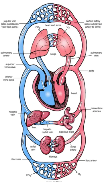
There are two pathways for the blood: the pulmonary and systemic circulation (fig. 1.2). In the pulmonary circulation, deoxygenated blood leaves the right ven-tricle of the heart via the pulmonary artery and travels to the lungs, then returns as oxygenated blood to the left atrium of the heart via the pulmonary vein. Instead, in the systemic circulation, oxygenated blood leaves the body via the left ventri-cle to the aorta and from there enters the arteries and capillaries where it supplies the body’s tissues with oxygen. Deoxygenated blood returns via veins to the vena cava, re-entering the heart’s right atrium where the systemic circulation ends. From a mechanical point of view the heart is considered as a pump, because it pumps blood through the entire circulation, to meet the requirements of all the cells of the body. The heart forces blood out of its chambers and relaxes to allow the next quantity of blood to enter. The contractions are named to systole and the relaxation diastole. Blood flows from an area of high pressure to an area of lower pressure. The myocardium is controlled by the electric activity of the heart that controls the timing of the heartbeat and the heart rhythm which is the synchronized pumping action of the heart chambers.

(21)

Figure 1.2: Circulatory System

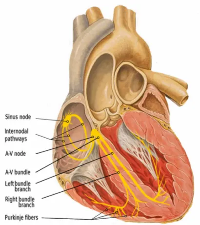
The heart conduction system consists of specialized cells, capable of generat-ing and conductgenerat-ing electrical impulses (fig. 1.3). It is composed by the senoatrial (SA), the inter-modal pathways, the atrioventricular node (AVN), the bundle of His and its branches and the Purkinje fibers. The heart beat begins when an elec-trical impulse is generated from the (SA) node, at the top of the heart. The signal than travels down through the heart, triggering first the two atria and than the two ventricles.

(22)

Figure 1.3: Heart Conduction System

The heart beat happens as follows:

1. The SA node generates an electrical impulse. 2. The upper heart chambers (atria) contract.

3. The Atrioventricular node (AVN) transfer impulse to the ventricles 4. The lower heart chambers (ventricles) contract and pump.

5. Than the cycle repeats itself.

The normal heart rate (HR) at rest ranges between 60 and 100 beats per minute. When the electrical pathway doesn’t work properly, heart rhythm problems may occur. Main cause of arrhythmias are due to alteration of activity of the SA node, the normal conduction pathway interruption or another part of the heart takes over as pacemaker. This leads to generation of cardiac arrythmias, some of them lethal like cardiac arrest of ventricular defibrillation.

(23)

1.2 Autonomic nervous system

The Autonomic Nervous system (ANS) main function is to regulate the activity of internal organs, usually involuntarily and automatically such as: blood vessels, stomach, intestine, liver, kidneys, bladder, genitals, lungs, pupils, heart, and sweat, salivary, and digestive glands (fig. 1.4). The autonomic nervous system is divided in two main branches based on its functioning, the Sympathetic and the Parasym-pathetic one. After the autonomic nervous system receives information about the body and external environment, it responds by stimulating body processes through the sympathetic branch, or inhibiting them through the parasympathetic one.

Figure 1.4: Autonomic Nervous System

(24)

Processes controlled by the autonomic nervous system are: Blood Pressure, HR and Breathing, body temperature, digestion, metabolism, balance of water and electrolytes, production of body fluids, urination, defecation, and sexual response. Most of the times, the two branches have opposite effects on the same organ. For example, the sympathetic branch increases blood pressure, and the parasympa-thetic one decreases it. Overall the two branches work together to ensure that the body responds appropriately to different situations.

Among the main functions mentioned above, the modulation of cardiac activ-ity is the one we are interested to focus on. In rest conditions the parasympathetic activity prevails, inhibiting the cardiac activity through the vagal activation, slow-ing down the HR. The sympathetic system instead, or the “fight or flight” reaction, is prevalent during the activities that require a fast reaction of the organism, incre-ments the HR and the strength of contraction to pump more blood in the circulation responding to a higher muscular activity.

The Sympathetic Nervous system (SNS) releases the hormones (catecholamines - epinephrine and norepinephrine) to accelerate the HR, instead the Parasympa-thetic Nervous system (PNS) releases the hormone acetylcholine to slow the HR. In absence of this external control, heart pacemaker cells discharge with a fre-quency around 100 bpm, but in resting conditions the frefre-quency is lower, around 70 bmp. This demonstrates that the parasympathetic activity exerts a higher influ-ence than the sympathetic one. During exercise or stressful activity the inhibiting behaviour of parasympathetic activity is deactivated and the sympathetic one starts increasing, increasing the HR and the blood pumped in the organism.

It has been observed that also in resting conditions, the HR fluctuates around an average rhythm. Such fluctuations are called heart rate variability (HRV). The SA node receives several different inputs and the instantaneous heart rate or RR intervals and its variation are the result of these inputs. Factors that affect the input are the baroreflex, thermoregulation, hormones, sleep-wake cycles, physical activity and stress. HRV has become an important risk assessment tool. A reduced HRV is associated with a poorer prognosis for a wide range of clinical conditions, while robust periodic changes in R-R intervals are often an indicator of health.

(25)

1.3 Heartrate measurements

To have in hand such information like HRV, first step to be done is to access the beat-to-beat activity of the heart. There are different methods to detect heart beats such as ECG, blood pressure, ballistocardiograms, and pulse wave signal derived from a photoplethysmograph PPG. Today’s most used and the standard for measuring the heart activity is the electrocardiograph (EKG) because it provides a clear waveform which makes it easier to exclude heartbeats not originating from the SA node. For the first time in history, the electrical activity was measured by the capillary electrometer developed by Gabriel Lippman. The different flex points on the graph were named A B C D. But the term EKG was used for the first time by Dr. Willem Einthoven, a Dutch physiologist to name the deflections on the measured electrical signal of the heart (fig. 1.5).

Figure 1.5: Two superimposed ECGs are shown. Uncorrected curve is labelled ABCD. This tracing was made with refined Lippmann capillary electrometer. The other curve was mathematically corrected by Einthoven to allow for inertia and friction in the capillary tube

(26)

From the first version as a string galvanometer electrocardiograph, improve-ments were made to make it more practical for clinical use. Earlier EKG recorded by Waller used five electrodes but Einthoven could reduce the number of elec-trodes to three by excluding those which he thought provided the lowest yield. He chose the letters PQRST for the corrected curve based on mathematical tradition of labeling successive point on a curve. In 1924, Einthoven was awarded the Nobel Prize in physiology and medicine for the invention of electrocardiograph. [2]

EKG is based on recording of electric potential generated by heart on body sur-face. Everything is based on depolarization and repolarization of cardiac muscle cells. These processes can be presented by vectors of electrical potentials. EKG is recording of summation of electrical potential vectors from multiple myocardial fibers, not only from cardiac conduction system. Every myocardial fiber generates electrical potential. These electrical potentials are conducted by body fluids to the body surface where they are recorded.

Each component of EKG waveform represents different electrical events dur-ing one heart beat. These waveforms are labelled P, Q, R, S, T and U. Among them, the most visible and easiest to detect is the R peak in the QRS complex which rep-resents ventricular depolarization and contraction. The instantaneous HR can be calculated from the time between two QRS complexes, or an R-R interval. To have an accurate measurement between two peaks, a good peak detection algorithm is needed, otherwise some error will be included in the time calculated and the HR variability will contain some erroneous information.

When the heart contracts, it pumps blood in the circulatory system generating a pulsatile waveform (fig. 1.6). This Blood volume pulse (BVP) is a signal highly correlated with the EKG. BVP is widely used as a method of measuring the HR because it is very easy to be applied in practice and has a low cost. Detection of these signal is done through photoplethysmography PPG. To better understand the principle of working of the PPG we should first consider the mechanical model of the heart and how the whole circulatory system behaves during a cardiac cy-cle, especially during the pulse phase. Heart is modelled as a compressible pump instead ventricles and atrium like chambers with some elasticity where volume and pressure varies during each cycle. This pressure wave travels from the aorta to the peripheric circulation where it is detected. In (fig. 1.6), we can see how pressure varies in the aorta during a heart cycle. On this cycle, two phases can be noticed. The ”anacrotic” one during which blood is pumped from the ventricles in

(27)

the aorta. It ends with the closure of the aortic valve and a small dip can be no-ticed on the graph representing the end of this phase. Then, the ”catacrotic” phase during the diastole during which blood pressure in aorta falls to the diastolic one. This wave travels to the peripherical circulation with its velocity of propagation and it changes a little bit the morphology due to the reflections from the branches of this system.

Figure 1.6: Blood volume pulse fluctuation in aorta.

The PPG measures the variation of the light absorbed due to the variation of blood flow in the peripheral circulation. The light traveling through the human body can be absorbed by different substances, including bones, tissues and venous and arterial blood as it can be seen in the (fig. 1.7). The majority of absorption is due to the continuous component which is the continuous absorption due to tissues and venous blood. The alternate component is caused by the absorption due to the arterial blood vessels that contain more blood volume during the systolic phase of the cardiac cycle than during the diastolic phase.

(28)

Figure 1.7: Absorption in PPG signal

Photplethysmographic PPG systems optically detect changes in the blood flow volume (i.e., changes in the detected light intensity due to different concentration of oxygenated hemoglobin). There are two types of systems: the transmission sys-tem and the reflectance syssys-tem as it can be seen in (fig. 1.8). In a transmission system, the light transmitted through the medium is detected by a photodetector opposite to the LED source. Instead in a reflectance system, the photodetector de-tects the light that is back-scattered or reflected from the tissues, bone and blood vessels [16]. According to the Beer-Lambert law, the change of blood volume in the tissue is reversely proportional to the intensity of the light reflected or trans-mitted from skin [20].

Figure 1.8: Two types of PPG systems

There are some disadvantages of PPG signals due to distance between the record site and the real cardiac cycle event, so the signal is less spatially and

(29)

porally defined. Despite the different nature of the signal in comparison with the gold standard EKG, PPG signals are still a good and a valuable source of informa-tion for measuring HR activity. Moreover, the BVP signal is totally non-invasive because it is recorded in the body surface, typically on the tip of the fingers or on the wrist. The latest developments in technology made possible the measure of variation of the light absorbed from the body due to variation of blood flow in the capillaries near to the body surface, with a camera. The applications and state of art on video PPG will be discussed in the next chapter.

(30)

(31)

Chapter 2 State of the art

Two primary advantages of in-contact PPG are the instrumentation’s low cost and the relative resilience to motion artefacts due to the physical contact between the subject and the sensor that suppresses relative motion. Recently non-contact pho-toplethysmography has become more popular (Humphreys 2007 [7] , Verkruysse et al 2008 [19], Poh et al 2010 [13], Kamshilin et al 2011 [1]) due to its comfort and convenience and minimization of infection risk in medical applications. The advantage of using a camera instead of a photoplethysmograph is that it allows to analyze multiple locations simultaneously, for example detect a PPG signal from multiple subjects or analyze the distribution of PPG signal over an area on a single subject.

2.1 Signal acquisition

With the video photoplethysmography technique the raw siganl where all the pro-cessing is done is the video signal of the skin surface. The instrumentation in most of the studies are conducted using CCD or CMOS cameras. In the first studies low resolution CMOS 24-bit RGB cameras with three channels 8 bit/channel with 15 fps were used for signal acquisition [13], [14] and in a later study a higher quality RBG camera with 100 fps was used[11] . There are also studies where they used monocrhome CMOS cameras [7], [1] at 20 fps. Most of the studies were con-ducted higher quality CCD cameras, some with RGB sensor [5], [9], from 20 to 60 fps and some with monochrome sensor [3] at 25 fps.

The studies done up to now can be categorized in two groups based on the light source used. The first studies were performed mostly using an external light

(32)

source. An fluorescent light source was used in [3] with an RGB camera. Led arrays with a fixed narrow band of wavelength emission were used in the exper-iments using monochromatic cameras as in [11], [7], [1] because the intensity of light reflected from the subject skin is modulated in time with different amplitudes based on wavelength. Later studies showed that it is possible to acquire qualitative video PPG signals also in ambient light conditions as in [19], [9].

Further development was done in this field on the later years by other studies where researchers tried to find out the best regions of interest on the subject’s skin and also develop better algorithms for motion tracking. The two regions of interest used mostly in the studies were the palm of the hand or the face. Most of the studies used the face as the best ROI since the capillaries are very close to the skin [14], [11], [19]. There are studies that used also the palm of the hand as ROI [7], [1].

2.2 Signal processing

The the Viola-Jones [18] face detection classifier algorithm is the most used when the ROI selected was the face. Some studies use the algorithm on each frame and this has a high computational cost [14], [5], [3]. To improve execution time some studies used a automated face tracker in the successive video frames [13], [9]. There is also a study where ROI was selected manually using a graphic user interface [19].

In most of the studies it was shown that there is a high time correlation between the green channel intensity and the light absorption by oxygenated-hemoglobin, more than with the red and blue channel. The latest approaches apply Indipendent Component Analysis (ICA) [14], [13] on the color channels of video recordings to extract a PPG signal. Other investigated methods rely on Eulerian video mag-nification (EVM) to detect subtle changes in skin colour associated with the pho-toplethysmography (PPG) signal [21]. There is also the Chromimance model [5] based on which it is possible to maximize the pulsating component of the reflected light and minimize noise by appropriate weighting the R, G and B channels.

In all forms of photoplethysmography, in particular when remote with no me-chanical coupling, motion artefacts can corrupt the signal such that the pulsatile waveform is irrecoverable. Nevertheless (Poh et al 2010 [8] ), showed that the average heart-rate from a long section of recording may still be possible to detect.

(33)

Any way, a worst case is when an artefact may be falsely detected as a valid PPG ‘pulse’. Several works were done on the artefact detection and reduction on PPG signals. Most of them perform motion artefact reduction in the cases of contact PPG sensors, coupling the PPG signals with the signal from an accelerometer or having a third reference signal of heart rate from EKG or other accurate measure-ment.

Various signal processing techniques have been investigated to address the problem of recovering quasi-periodic PPG signal from data corrupted with mo-tion artefacts. These include Wavelet analysis and decomposimo-tion techniques [12], adaptive filters [8] where non-linear phase filters, induce distortion on the PPG sig-nal in the time domain, but it doesn’t affect detection of heart rate. There are works involving analog filters and moving average techniques [15]. The artefact separa-tion problem has been viewed also as a blind source separasepara-tion problem by Yoo et al [10], [11] where enhanced preprocessing unit preceded the ICA block. The preprocessing unit consisted of detection of periods of signal using an autocorrela-tion method followed by a block-interleaving operaautocorrela-tion. However, this technique relies on the ability of the autocorrelation technique to correctly detect the wave-form period and hence provides erroneous results in presence of extreme motion artifacts. In the work by Elfadel et la [6] it was used a technique based on the use of correlation canceler for correlating and cancelling motion artifact signals (secondary signal), then the primary signal is used for measuring the heart-beat rate. However, the accuracy of this technique relies on the ability to accurately determine the proportionality constant and the secondary reference signal.

As mentioned above, in the case of non-contact video PPG signals PPG, sep-aration of valid signal from noise is more difficult. Subject movements and light changes lead to low Signal to noise ratio (SNR) of the extracted video PPG signal. The most common approach is the use of the frequency domain for the heart rate detection. The Fast Fourier transform (FFT) or the short-time Fourier transform (STFT) is applied by sliding a temporal window through the raw or preprocessed video PPG signal in the works by Dong et al in [11]. In the work by Andreotti et al [3] they used of Kalman Filtering to reduce the RMS error of estimated heart rate, increasing the detection accuracy. Some signal quality indexes were calculated to be used as inputs to the Kalman Filtering. Also in this case, to obtain these signals a reference finger BVP signal was used. This work was based on mostly on the protocol of the aforementioned paper, but we focused on finding a way to classify

(34)

between good and bad signals, without having any reference signal.

(35)

Chapter 3 Experimental protocol

The starting point of this work was to recover heart rate signals through a webcam and ProComp finger PPG. We acquired 3 minutes and 5 seconds synchronised signals of subjects with a webcam positioned 0.5 m in front of them. The subjects were in sitting position. They had to follow a protocol during which they had to follow a video presentation and than do some tasks on the pc. Meanwhile also the finger BVP signal was acquired from the index finger on the left hand. The idea of this protocol was to simulate our daily working position and behaviour on the pc.

3.1 Study population

We acqired signals from 25 subjects, 19 of which were students of Politecnico di Milano and 6 were high school students. All subjects are healthy without a history or diagnosis of any cardiac disease. Most of them were non-smokers, only two are occasional smokers. Their average age is 22 ±3 years and the gender distribution is 13 females and 12 males. All the subjects underwent the experiment willingly.

3.2 Equipment for signal acquisition

To make the acquisitions the following equipment was used: • 1 Desktop PC with i7 processor

• 1 Laptop PC

(36)

• 1 tripod

• 1 Technology Flexcomp-Infiniti sensor system for BVP • Biograph infiniti software

• OpenCV libaray written in C++ for video recording • White paper with shape of small circle

• Light paper sticker

The webcam and Thought Technology Flexcomp-Infiniti sensor were con-nected to the Desktop PC. The Laptop was used to show a Power-Point Presen-tation and to simulate the normal working routine on the PC. A white small paper circle was attached on the front, in between the eyebrows of each subject. This was done to validate the face tracking algorithm with by comparing it with the circle tracking.

Figure 3.1: Acquisition setup

(37)

3.3 Signal acquisition

Subjects were seated in a chair, with the left hand immobile on the table in front of them where was also the Laptop PC. Flexcomp-Infiniti BVP sensor was placed on the index finger of the left hand (fig. 3.1). The webcam was placed on a tripod in front of the subject, just behind the Laptop screen, 50 cm from the face. It was placed there and not on the laptop screen, to avoid some extra movements while subjects performed the tasks on the pc. The experiment was performed indoor and the light source was a mixture of natural light entering from the window and artifi-cial fluorescent-tube light. The BVP acquisition was initialized first from Biograph infiniti software and 1 second later the Video Recording. BVP was recorded at 256 hz, instead the video was recorded with a frame-rate of 60fps and a resolution of 1280x720 pixels.

The experiment was divided in two main parts where all the subjects were asked to sit relaxed and to act naturally. During the first part, they had to follow the instructions on a Power Point presentation for 1 min and 20 seconds. During this time, they had to follow the movement of a red circle with their head, (not only the eyes) on the screen in their natural way. Immediately after this short video, in the second part they were asked to do some tasks on the pc only with their right hand, so time to time, they had to move their head up and down to see the keyboard. They were asked to do some search on Wikipedia and read the definition of the asked question. On the remaining part, they played their favourite song on YouTube and follow the rhythm with small movements of their head as they would do when listening to music on their pc. We acquired 5 seconds extra so we could truncate the signals to have both of them synchronized.

(38)

(39)

Chapter 4 Signal Extraction and Processing

After signal acquisition we have two signals to elaborate: • Video registration

• Finger BVP signal

Theses raw signals need to be processed to extract useful information from them.

4.1 Signal extraction

The software used for extracting the raw signals from the video recording were MatLab and some OpenCV libraries written in C++ programming language by L.Iozzia et al [9]. All videos were recorded with Python. The code used to pro-cess the video signals used the Viola-Jones classifier algorithm to detect the face regions of interest (ROIs). The Regions of interest in our case were the forehead, cheeks and nose (fig. 4.1). Lucas-Kanade-Tomasi (KLT) algorithm was used to track the regions independently for a faster execution and more stable measure. To have a more reliable signal from the ROIs, face detection algorithm was initialized 10 times during the video sequence, because in presence of fast movements, the tracking algorithm didn’t perform well.

As output of from this first processing phase, 4 comma separated values (CSV) files were created. The first file fps.csv contained the time stamp of each frame that is used later to do the interpolation of each frame to equally space them in time. The second file motion, contained x and y coordinates of tracking of all ROIs.

(40)

Every two columns contained the x y coordinates of the center of the ROIs and the two last columns contained the coordinates of the center face position. The rows represent the evolution of the position on each frame of the coordinates. These signals were used as a quality index for the video PPG signal as the movement of face position during the video signal acquisition is directly linked to the quality of the signal obtained. The last file rgb.csv contained R,G,B average signal from the pixels inside each ROIs. Information from all the channels was used to improve the quality of the green channel as it was the one with the best quality where the BVP signal was more visible [9].

Figure 4.1: Video signal being processed by the OpenCV software. Tracking points and ROIs are visible on the picture

A MatLab code was written to track the circle attached in between the eye-brows, down the forehead of each subject. As output we had the x, y coordinates of the circle on each frame. This signal was used after to validate the face tracking algorithm of the OpenCV. The finver BVP singals were extracted from the

(41)

graph infiniti software on a text file that contained time and the intensity of BVP signal for each sample.

4.2 Signal Processing

On video pre-processing, signals are extracted on Python with the OpenCV li-braries written on C++. These raw signals showed some discontinuity due to the reinitialization of the face tracker algorithm. The post-processing phase is done on MatLab. After importing the signals in the MatLab environment, as a first step, the signal was detrended. Because of the slight variation of light intensity in normal conditions of the experiment, there was also variation of the sampling frequency of the webcam. So as a second step we interpolated the signal with the new time stamp to have them equally distant in time. The signal we are interested in, the video PPG has spectral components in a narrow band of interest between [30-300 bpm] or in frequency [0.5-5] Hz. We filtered all the information out of [0.5-5] Hz with a zero phase butterworth 4thorder filter (fig. 4.2).

Figure 4.2: Raw Video PPG signal and the detrended, filtered version

(42)

A method developed and implemented in our lab by L. Iozzia et al [9] was used for the next proccessing phase of the video signal. It consists in the chrominance model and the ICA method. The chrominance model is used to reduce the ef-fects of light variations and achieve motion robustness in the assumption that these external sources of noise modify all the three RGB channel equally. It is used to enhance the second channel signal, (green one) from the information of other chan-nels. The ICA is a statistical method for transforming a multidimensional random vector into components that are statistically as independent as possible from each other. The method assumes that the observed signals are a linear transformation of the sources y(t)=Ax(t). The aim is to find the inverse of the mixing matrix A called demixing matrix W as ˆx=Wy(t).

A lot of transformations are done to the initial data to find the demixing matrix and the order of the vectors is changed. The reason why the ZCA is used instead of ICA is to maintain the output data as close as possible to the original one. A better mathematical explanation can be found in the article [9].

Figure 4.3: Power Spectral Density of Video PPG signal calculated with Welch’s method

(43)

All these steps were done to filter out as much noise as we can from the desired signal. Then based on the work done by Andreotti et al [3], the signals were divided into 10 second segments with 5 seconds overleap. Each signal was long 3 minutes. After this segmentation we had (2x180/10)-1=35 segments of 10 seconds for each subject.

The transformation from the time domain to the frequency domain were done through a non-parametric form, the discrete time Fourier transform (DFT). The Hamming window and zero padding was applied on the initial signal to have a better and smother signal in the frequency domain(fig. 4.3).

Figure 4.4: Raw face tracking signal and the detrended version

For the tracking signal extracted on the same way the first pre-processing steps were the same. First, it was detrended because of the discontinuity it had due to the re-initialization of the face tracker algorithm. After an examination of the fre-quency components of the tracking tracking signal, the same butterworth 4thorder filter was applied to eliminate some noisy components present in the signal not

(44)

lated to the movement (fig. 4.4). The signal was brought on the frequency domain through the DFT transformation with a Hamming windows and zero padding as well.

The finger BVP signal extracted from the Infinity software had to be detrended and filtered as well in the same way. After this phase, it was calculated its PSD with the DFT transformation using a Hamming window and zero padding.

The circle tracking algorithm was all written in MatLab. It calculated the x and y coordinates of the center of the white circle in each frame. To reduce the pro-cessing time, only on the first frame the algorithm searched for the location of the white circle. In each successive frame, a small area was cropped around the known location of the square from the previous frame and the search was performed only in this area. As output we had the x and y coordinates of the centre of the circle. This information was used to validate the face tracking algorithm.

(45)

Chapter 5 Feature extraction and Classification

After reducing the noise of the signals and transforming them in different domains, feature extraction and selection was performed. It is very important to reduce error in each step of our work, not to carry useless information and corrupted data for the classification algorithm. Some of the features extracted during the pre-processing phase were discussed also in the previews chapter.

5.1 Feature extraction

Most of the work was done in the frequency domain. Many parameters were cal-culated to obtain as much information from these signals. For the Video PPG signal the first parameter to calculate was the peak on the power spectrum den-sity PSD representing the main frequency component related to the heart rate. In some cases, because of the noise present on the band of interest, the PSD didn’t have a single peak and it was impossible to detect the heart rate pulse form such a spectrum. After this, the second parameter to be calculated was the percentage of power in the first harmonic of the PSD. This peak density is computed as the ratio between the integral of the PSD in a band around the dominant frequency peak [fD± ∆f ] and the overall PSD of the signal representing the Signal to noise ratio

(SNR) (fig. 5.2). SN R = PfD+∆f fD−∆f|X(k)| 2 Pfmax fmin |X(k)| 2

(46)

where the values are 0.25 of the maximum value. We used this parameter as an in-dex for the classification to choose between noise artifact and noise free segments (fig. 5.1) .

Figure 5.1: Power spectral density of Video PPG signal. On grey is the power under the main lobe up to 25% of the Peak

Figure 5.2: Features extracted from the rgb.csv file

(47)

For the tracking signal some time-domain features were calculated such as the mean velocity, the maximum velocity and the standard deviation on each [10 sec] segment. In the frequency domain there were calculated the power, as the cumu-lative sum of the PSD. The peak of the power spectrum was calculated as well, so we know if there is any relation of the frequency movement and its influence in the video PPG, since maybe some frequencies may affect more and some less our signal of interest (fig. 5.3).

Figure 5.3: Features extracted from the motion.csv file

The finger BVP signal in our case was considered as reference signal, so the noise was much less than other signals. In the frequency domain, the peak of the power spectrum representing HR frequency was calculated. Finger BVP is considered a good signal for reference for HR measurements.

The frequency difference between the peak frequency of the Video PPG signal and the peak frequency of the power spectrum of tracking signal was the last fea-ture, calculated as a ratio between two other features previously calculated. This feature was calculated under the assumption that there should be some connection between the two frequencies when the artifact movement interferes in the Video PPG signal. This had to be verified in the following steps.

Other parameters we could try to measure in our work were the skewness and kurtosis of the power spectrum of video PPG, but considering our signal had al-ways some noise components, it was impossible to decide about this parameter, in such a noisy signal.

(48)

5.2 Labeling

The main objective of the classification is to distinguish between artifact and noise free signals from video PPG. The finger BVP signal is used as reference to check if the peak on the power spectrum of video PPG is similar to the peak on the power spectrum of finger BVP. For each subject, a match vector is created. The match was set to 1 if the peak in both power spectrums differs with less than 0.2 Hz, that is a normal deviation due to HRV in the respective segment and the small difference in some cases [1 s] of signals in time respect to each other. As second criteria was set also the SNR, and the requisite was that the SNR should be >0.4 of the total area (fig. 5.4). The artifact movement introduced a lot of noise on the power spectrum of Video PPG. It is necessary that the main peak should be distinguishable from the other peaks maybe present in the power spectrum. After having this match matrix for each subject, the further steps for creating a supervised classification algorithm were implemented.

Figure 5.4: Labeling decision flowchart

(49)

5.3 Normalization

Even though all the subjects followed the same protocol during the signal acquisi-tion there were some variaacquisi-tions in between the subjects. For a better performance of the classification it is necessary a normalization phase. For our purpose the best is the feature scaling normalization or the so-called unity-based normalization.

Xnorm =

X − Xmin

Xmax− Xmin

After a deeper look on the data distribution, it was noticed that the max value in some subjects was much greater than in others. This was affecting all the data on that subject. To avoid such bias on the data the features were selected, instead of Xmax− Xminvalue in the formula, there were chosen the average values among

all the subjects. This helped to have more uniformly distributed data for the clas-sification process.

5.4 Feature statistics

For each feature extracted from the signals some statistic was performed. The data were divided in two groups based on their Label class. First it was studied if the data come from a normal distribution. As it can be seen for the case of mean velocity of tracking (fig. 5.5), the distribution of data normalised data is not a normal distribution. The Lillieforst Test was performed for each feature and it was observed that the data in all cases were not normally distributed. Data distribution depends on the experimental protocol. In our case, the subjects performed a lot of movement during all the acquisition and only few seconds they were not moving.

(50)

Figure 5.5: Normalized distribution of mean velocity of tracking

Some tests were done to measure the discrimination capacity of each feature. As it was seen in the previews test, each feature was not normally distributed. In this case, the two-sided Wilcoxon rank sum test was performed. It is a non-parametric alternative to the two-sample t-test, and it is used when the population cannot be assumed to be normally distributed. It is used to determine whether two dependent samples from the population are having the same distribution or not. The Null Hypothesis (H0) is that the data are samples from distributions with equal medians. In all cases the test results were equal to 1, with a p-value <<0.05, meaning that the null hypothesis was rejected. All the features were ordered based on the p-value of the Wilcoxon rank sum test, from the smallest to the largest value based on their discriminating capacity. The results of the Weicoxon test showed low p-values but this didn’t exclude the fact that there is quite a lot of overlapping between the two classes of each feature.

(51)

5.5 Correlation between features

It is fundamental to know the relationships between different features: for instance if two or more indexes are correlated because using them simultaneously is a re-dundant operation which can negatively affect the efficiency of the classification process. A study on the correlation between features is performed and it was shown that there was a strong correlation between some of them. For example, the standard deviation (SD) is correlated to the PSD since the latter is the description of the variance in the intervals distributed over the frequency spectrum.

Also the mean velocity over the signal segment is highly correlated with the SD. They are linearly correlated as it can be seen from the (fig. 5.6). The exception are on the small values where the mean value of velocity can be close to zero, instead the SD gets higher values. In general, the correlation matrix among all the features was calculated and the results are shown below. Beside the graphical visualization of the correlation in between features, the correlation matrix was calculated as well to have a better idea.

Figure 5.6: Correlation between SD and Mean Velocity of tracking signal segments

(52)

In medical applications, it is very important that the data you analyze are mean-ingful for the application in hand. Noisy data may induce erroneous information for the patient and so treating the condition not in the right way. The most im-portant thing in any medical application is not to aggravate the patient’s condition, than if it is possible to improve his health.

(53)

Chapter 6 Classification and Results

In the previews chapters, different features were extracted and their discrimination capability was estimated. In our experiment, univariate analysis cannot discrimi-nate very well between noise free and artifact signals because the values of a single feature overlap in most of the cases. A more appropriate solution to this problem could be a multivariate analysis.

6.1 Support Vector Machine

A support vector machine (SVM) is a decision-making method which takes into account multiple indexes to operate an automatic classification into classes and it is can solve problems of big dimensions [17]. A SVM classifier performs the identification of hyperplanes defined by these support vectors which represent the target classes, and are used to classify the observations into one or more cate-gories. In our case a multivariate analysis based on the n-features extracted is performed. Every segment of windowed signal is represented by an n-dimensional vector. Each segment is seen as a point in a n-dimensional space. Therefore, the classification of each segment is computed as a problem of spatial separation among n-dimensional points by the SVM algorithm. The algorithm operates a par-tition among those points through the use of separation hyperplane. For example, if we have to distinguish between categories on the basis of two indexes, the sepa-ration plane can be visualized as a straight line that is used as a frontier which best segregates the two classes. (fig. 6.1).

(54)

Figure 6.1: Linear SVM classification in 2D space

Adding one more features to the classification, the problem evolves first to a 3D model where a plane will divide the data in two classes. In our case there are 9 features, so there is not a graphical representation of the problem solution.

As a preliminary operation for the correct performance of the SVM classifier, the features need to be normalized, because features with greater range of values tend to have bigger weight in the decision process. So normalization is done to en-sure that every parameter has the same relevance in the classification process. The SVM is an example of supervised learning. Meaning that the algorithm goes first though a training phase with a portion of the data set, called training set. The train-ing set is made of labelled data as artifact or motion free data. The performance is evaluated trough the leave one out cross-validation method.

Based on the work by Dash et al [4] among the methods for feature selection, a “wrapper method” (the classifier is the evaluation function), was chosen for feature selection. The features selected using the classifier that later on uses these selected features in predicting the class labels of unseen instances, the accuracy level is very high although computationally quite costy.

(55)

The classification model used for feature selection is the linear discriminant classification. The choice to use this classification model was made in order to reduce the time of computation on each cycle. For each feature, it was calculated the confusion matrix of the classification model. On each cycle, it was chosen the feature giving the highest performance. After choosing the feature with the highest performance, another feature was added and the performance is calculated again making all the combinations of the first feature with the rest. If the performance of two best features is higher than only with a single one the process was repeated, adding more features to the discriminant classification algorithm, until there is no more improvement in performance. To measure the performance, it wasn’t taken in consideration the accuracy but the false negative rate (FNR) as we want to reduce the causes when a noise is considered as heart rate frequency.

F N R = F alse positives

F alse positives + T rue positives

At this point, out of 9 features initially extracted, we selected 5 of them. They were saved in a new variable and ordered based on their impact on performance of the classification algorithm. The features selected are:

• Frequency of video PSD peak

• Frequency length of main lobe of Video PSD

• SNR

• Difference frequency peaks of PSD of Video and Tracking signal

• Max velocity tracking

To better understand their importance on classification, a parallel coordinate plot with quantile values of the selected features was done (fig. 6.2). In the figure is shown the median values of each feature with 25% of quantile values.

(56)

Figure 6.2: Parallel plot of features selected to be used for the SVM classifier

As it can bee seen, there is a lot of overlap between the two classes of each feature.

With the selected features a Quadratic SVM was trained. It was chosen the Quadratic SVM because it was observed that for each feature the division in be-tween two classes most of the times was not like a straight line but more like a quadratic one. It is also tested in an iterative way that the best performance is reached through the quadratic SVM classifier.

6.2 Results

The initial data-set was divided in the training set that we used to build the classifier and into validation set. This second part was used to measure the performance of the classifier on the unknown data, not related to those used for the training phase. The initial performance of the classifier was quite low, with an accuracy = 84%.

A more deep study was done on the data-set and it was observed that some 38

(57)

subjects did many movements during the acquisition, and there was some noise also in the finger BVP signal that was used as a reference. To overcome this problem, 5 more acquisitions were performed in order to substitute the noisy ones. This change increased the performance of the classifier. To further increase the performance an other feature was added, the wideness of the main lobe of the Power Spectrum indicating how good the power is concentrated in this narrow band of frequency. The more narrow the band is, the better should be the quality of the signal and vice-versa. With these two interventions the performance of the Quadratic SVM classifier increased. The results of this Classifier are shown in the Confusion Matrix below (fig. 6.3).

Figure 6.3: Confusion Matrix of the quadratic SVM classifier results

The target class are the Labeled data from the Validation data-set. The Output class are the data predicted from the quadratic SVM classifier. As it can be seen, the accuracy = 94.5% and the FNR = 6.6%.

An other method was used to be compared with the Quadratic SVM. Since in many articles the Feed-forward Neural Network was used as a method for classifi-cation, I trained and tested a similar method with the same database. After all the

(58)

necessary steps this method showed a lower performance respect to the Quadratic SVM one as it can be seen in the table 6.1.

Quadratic SVM

Feed-forward Neural Network

accuracy

94.5%

78.1%

sensitivity

96.2%

90.2%

specificity

93.4%

61.4%

Table 6.1: Classification performance

Some further analysis was done to understand better the cases the classification was done wrong. A visual inspection was done on each signal segment in the time and frequency domain. Despite all the work done to clean the signals from the artifact noise some signals were still not useful for the heart rate detection. During the protocol of signal acquisition, around the end of the first minute subjects had to perform quite fast movements with their head. That was the part when the algorithm could not get useful information from the video processing.

Figure 6.4: 10 [sec] segment of artifact signal in the time and frequency domain

(59)

As it can be seen in the fig. 6.4 the power of artifact noise in the band of interest is much higher than the heart rate one. The subject was performing periodic move-ments with his head and as a result there was that peak in low frequency. It can be seen also in the time domain that it is impossible to extract useful information from such noisy signals.

It was more interesting to observe the border condition between bad and good signals. On each feature considered for the classification there was over-leap be-tween the two classes it had to discriminate, so even using multiple features for the classification there was still some error in the results. The main cases of er-ror were when the segment was classified as valid for heart rate extraction, but in the previews phase we labeled that signal as not valid since we left some margin of robustness in the cases we considered good ones for heart rate extraction. As it can be seen in the fig. 6.5 the main peak of the power spectrum represents the heart rate with a difference respect to the finger BVP measurement of 0.03 Hz and was classified as good one, but I considered this as not valid because the power of artifact noise is very close to the heart rate one and this case should be avoided.

Figure 6.5: 10 [sec] segment of low noisy signal in the time and frequency domain

In most of the cases the signal was considered a good one for the heart rate 41

(60)

extraction. In the frequency domain ti could be observed a very high single peak representing the heart rate frequency and also in the time domain there was very high similarity in shape with the BVP signal fig. 6.6.

Figure 6.6: 10 [sec] segment good signal in the time and frequency domain

The overall results are acceptable but further improvement can be done. This will be discussed in the next chapter.

(61)

Chapter 7 Discussion

7.1 Discussion

The photoplethysmography BVP signal can hold valuable information about the health of a patient. To access this information in clinical conditions is much easier than in daily life conditions. This thesis tested the ability to acquire reliable photo-plethysmography BVP signals from the video captured with a web-cam simulating daily life conditions. The results show that there is still a lot of work to be done to improve the acquisition technology, such as reducing the noise due to movement. Beside that, there is some noise also due to the variation of light intensity because of the acquisition conditions. While subjects followed the acquisition protocol, the face angle with the light source varied and so also the light intensity on their face, introducing more noise on the signal. Our work consisted mostly on detec-tion of these noisy signals that can not be used to evaluate heart rate. The features selected to do such discrimination were chosen so in any possible implementation of video PPG acquisition, it is possible to extract such values without the need of other reference signals.

There is still to be decided about the limits whether to consider the signal still valuable for HR detection or not. In my case I stabilized those limits after manually checking the PSD of each segment. In a more wide application of such a method to classify in between good or bad signals we should be more restrict about the limits depending also in the type of application.

(62)

7.2 Limitations and future work

The overall results showed that among 20 subjects and 35 signal segments for each = 700 signal segments only 273, about 39% were considered valuable to access the HR information. The protocol used to do the acquisitions had a lot of movement, maybe over-simulating normal movements we usually do while working on a pc. The method developed in our lab [9] will have a better performance in daily life conditions. Something that could be improved on our project is the length of the acquisition for each subject and use a more relaxed protocol for the subjects to follow.

The face tracking algorithm showed some difficulty to track the ROIs. In gen-eral there was very high similarity between face tracking algorithm used in the OpenCV library written in C++ and the validation circle tracking as it can be seen in the figure below (fig. 7.1).

Figure 7.1: X and Y coordinates of tracking from the face tracking algorithm and the circle tracking used for validation

(63)

This is a preliminary work to identify between valuable signal and noisy ones to access the heart rate information. Much optimization and normalization work should be done to implement this method on a wider range. The classifier we build can discriminate in between the signals acquired under those predefined condi-tions, since it uses information that is sensitive to the geometry of the camera and position of the subject. More information should be included in order for the al-gorithm to be implemented in other devices such as camera model, so by knowing the opening angle and other characteristics of the acquisition, we can predict the distance of the subject from the camera and the area of our regions of interest. This information should be included in the normalization phase in order for the algorithm to perform better.

(64)

(65)

Greetings

Beside the study experience, these years were a very valuable life experience for me. During this time I met a lot of special people and ”beautiful minds” I would call, that influenced a lot on my formation. I would like to thank all the professors I met in Politecnico. Each of them was special in its own way. Waking up every morning and coming to classes of professors ”humans” that decided to share their knowledge with others was a joy for me (most of the time).

I would like to thank all the people that I met on this long journey of studies in Politecnico di Milano, which later became my friends. Some of them became my family. I would say thank you to Pocho, ”Zhora” and Ben for the great time we had when studying and living together.

I would thank also my Albanian friends Andi, Endi, Gesoo, Genti and c¸unat for the support and great times we had. I know this experience in Milan wouldn’t have been this beautiful without all of you.

A special thank goes to Piero and Paolo and all the guys I worked with during these years. The hard work during all the exhibitions and the great time of all the concerts we worked in, can not be forgotten.

Last but not least I thank my family, the most important part of me, for their support and advice. No matter the time and distance we always kept our relation strong and with love.

(66)

(67)

Bibliography

[1] Kamshilin A. A., Miridonov S., Teplov V., Saarenheimo R., and Nippolainen E. Photoplethysmographic imaging of high spatial resolution. Biomed. Opt. Express, (2):996–1006, 2011.

[2] Majd AlGhatrif and Joseph Lindsay. A brief review: history to understand fundamentals of electrocardiography. Community Hosp Intern Med Perspect, pages 201–213, 4 2012.

[3] F. Andreotti, A. Trumpp, H. Malberg, and S. Zaunseder. Improved heart rate detection for camera-based photoplethysmography by means of kalman filtering. IEEE 35th Int. Conf. on Electronics and Nanotechnology, (35):428– 433, 2015.

[4] M. Dash and H. Liu. Feature selection for classification. Intelligent Data Analysis, 1:131–156, 5 1997.

[5] Gerard de Haan and Vincent Jeanne. Robust pulse-rate from chrominance-based rppg. IEEE Trans. Biomed. Eng., (60):2878–86, 5 2013.

[6] M. K. Diab, E. Kiani-Azarbayjany, I. M. Elfadel, R. J. McCarthy, W. M. Weber, and R. A. Smith. Signal processing apparatus. U.S. Patent 721 598, 4 2007.

[7] Humphreys K. G. An investigation of remote non-contact photoplethys-mography and pulse oximetry. PhD Thesis National University of Ireland, Maynooth, 2007.

[8] J. M. Graybeal and M. T. Petterson. Adaptive filtering and alternative calcula-tions revolutionizes pulse oximetry sensitivity and specificity during motion and low perfusion. Proc. 26th Annu. Int. Conf. IEEE Eng. Med. Biol. Soc., 2:5363–5366, 9 2004.

(68)

[9] L. Iozzia, L. Cerina, and L. Mainardi. Relationships between heart-rate vari-ability and pulse-rate varivari-ability obtained from video-ppg signal using zca. Physiological Measurement, 37(11):1934–1944, 9 2016.

[10] B. S. Kim and S. K. Yoo. Motion artifact reduction in photoplethysmog-raphy using independent component analysis. IEEE Trans. Biomed. Eng., 53(3):566–568, 3 2006.

[11] L. Kong, Y. Zhao, L. Dong, Y. Jian, X. Jin, B. Li, Y. Feng, M. Liu, X. Liu, and H. Wu. Non-contact detection of oxygen saturation based on visible light imaging device using ambient light. Opt. Express, 21(15):17 464–71, 6 2013. [12] MS. Lee, B. L. Ibey, W. Xu, M. A. Wilson, M. N. Ericson, and G. L. Cote. Processing of pulse oximeter data using discrete wavelet analysis. IEEE Trans. Biomed. Eng., 52(7):1350–1352, 6 2005.

[13] Poh M-Z, McDuff D J, and Picard R W. Non-contact, automated car-diac pulse measurements using video imaging and blind source separation. Biomed. Opt. Express, (18):10762–74, 2010.

[14] M.-Z. Poh, D. J. McDuff, and R. W. Picard. Advancements in noncontact multiparameter physiological measurements using a webcam. IEEE Trans. Biomed. Eng., 58(1):7–11, 1 2011.

[15] J. E. Scharf, S. Athan, and D. Cain. Pulse oximetry through spectral analysis. Proc. 12th Southern Biomed. Eng. Conf., pages 227–229, 4 1993.

[16] T. Tamura, Y. Maeda, M. Sekine, and M. Yoshida. Wearable photoplethys-mographic sensors — past and present. ACM. Transactions on Graphics, 3(2):282–302, 4 2014.

[17] C. Vercellis. Business intelligence. McGraw-Hill, 2006.

[18] P. Viola and M. Jones. Rapid object detection using a boosted cascade of simple features. Proc. of IEEE Conf. on Computer Vision and Pattern Recog-nition, pages 1063–6919, 12 2001.

[19] Verkruysse W, Svaasand L O, and Nelson J S. Remote plethysmographic imaging using ambient light. Biomed. Opt. Express, (16):21434–45, 2008.

A classification method for noisy video PPG signals detection

POLITECNICO DI MILANO