Dynamics of supercooled aqueous systems at low temperature and high pressure.

U

NIVERSITÀ DEGLI

S

TUDI DI

P

ISA

Facoltà di Scienze Matematiche Fisiche e Naturali

–––––––––––––––––––––––

2008-2010

Ph. D. Thesis in Applied Physics

Dynamics of supercooled aqueous systems at

low temperature and high pressure

Candidate

Supervisor

Sergiy Ancherbak

Dr. Simone Capaccioli

Abstract

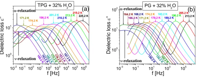
Aqueous mixtures are excellent systems to deepen the understanding of the relaxation dynamics of supercooled water in the temperature region usually unaccessible without crystallization. The first part of this thesis provides an investigation, by means of dielectric spectroscopy, of the molecular dynamics of water mixed with propylene glycol oligomers (n-PG, n = 1, 3, 7) at ambient and extremely high pressure (up to 1.8 GPa). By changing in a systematic way the relative concentration of water (starting from small amount of water, 2.0 wt.%) added to polypropylene glycol, PPG400, three relaxation processes show up: a) the slowest process, whose dynamic properties indicate that it is the structural α-relaxation of the aqueous mixture leading to glass transition at T equal to the calorimetric Tg; b) a faster process (ν-relaxation

process), which appears close to β- (secondary) process of PPG400 in dielectric spectra even for the lowest water concentration mixture (similarly as in the case of many other water mixtures) and has the characteristics of an intermolecular Johari-Goldstein secondary relaxation; c) the fastest process (γ-relaxation process), originating from hydroxyl group rotation, which is prominent for anhydrous PPG400, but this process is weak and becomes hidden by the much stronger ν-relaxation for high water concentration mixture.

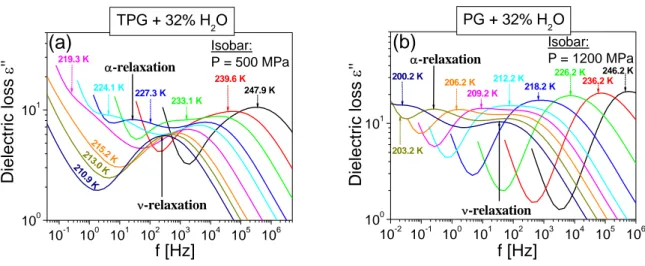
In addition, a change of the dynamics of the water related (ν-) process occurs in all isobaric measurements: the temperature dependence of ν- relaxation time, τν, that has an Arrhenius

behaviour in the glassy state, becomes stronger on increasing temperature in the liquid state. Such a crossover is in a way significantly different from similar phenomenon observed in literature for confined water. Moreover, our studies under pressure revealed that the secondary relaxation process for aqueous mixtures of PPG400 with low (4 wt.%) and high (26 wt.%) amount of water behaves in a different way. Our results show that the secondary relaxation in the mixtures with low content of water is mainly influenced by the dynamics of the solute molecules and has the characteristics of the Johari-Goldstein β-relaxation occurring in van der Waals and polymeric glassformers. In the case of high water content, where each molecule of water is mainly surrounded by other water molecules, the ν- (secondary) relaxation has very specific characteristics, quite different from those of conventional glassformers in its ability to rotate and translate after breaking two hydrogen bonds.

Finally, mixing water with n-PG oligomers (increasing the number of repeating units, n) with similar weight concentration of water allowed us to study how the dynamics of water mixtures at ambient and elevated pressure is influenced by the number of OH-groups and by the connectivity of the solute. Similar studies have been carried out for aqueous mixtures with ethylene glycol oligomers.

Among the numbers of new experimental findings coming from this work, three results can be mentioned, of particular interest for the current debate in literature on dynamics of aqueous systems. The first is the increasing of timescale separation between α- and ν- process in dielectric spectra at given (the same) α- relaxation time, τα, on increasing temperature and pressure. This

behaviour is usual for the timescale separation between α- and β- processes of hydrogen bonded systems (like sorbitol) and not shown in the case of van der Waals liquids where the α-β timescale separation is the same on increasing temperature and pressure but keeping constant τα.

This effect is related to the fact that the H-bond network in such systems is weakened by elevating temperature and pressure and the structure of the system is changing with the thermodynamic conditions.

The second result of particular interest is that, when it has been possible to clearly reveal the ν-relaxation from the glassy state up to well above Tg, a strong deviation from the glassy state

trend has been found for both the temperature and pressure dependence, with an apparent kink in the relaxation map always occurring near the glass transition of the aqueous mixtures. The only explanation for such result could be that such crossover in temperature or pressure dependence of ν-process is related to glass transition. This occurrence helps to rule out some of the hypotheses on dynamic crossover recently published in literature.

The third important result is that the dielectric strength of the water-specific relaxation also exhibits a crossover from a weaker to a stronger dependence with increasing T, at the temperature where the slow process attains a very long timescale (> 1 ks) and becomes structurally arrested.

All these facts support the idea that water-specific ν-relaxation can be identified as the Johari-Goldstein β-relaxation of water. This interpretation of ν-relaxation is in full agreement with the temperature, pressure, concentration dependence of its dynamic features and dielectric strength. Taking into account the experience gained from the work on aqueous mixtures of glycol

mixtures with saccharides or carbohydrates (mono-, di- and polysaccharides). The main idea was to investigate, by means of dielectric spectroscopy, the dynamics and glass transition phenomena of water-sugar mixtures under pressure for possible application to cryoprotection, food preservation, biological functioning of hydrated biomolecules. In order to widen the possible applications of this study, sugars of strong interest in bio-science were chosen, such as fructose, glucose, sucrose, trehalose, dioxyribose, glycogen. For water-fructose solutions a systematic study was done in a wide pressure range by varying concentration of water. A preliminary study of the dynamics of proteins solved in sugar-water mixture was also begun.

Summarizing, our results show that the relaxation time of the ν-process, τν, represents

qualitatively very similar features for all studied aqueous systems, almost universal, irrespective of the chemical and structural differences, especially for high water concentration mixtures. The

ν-relaxation has an Arrhenius T-dependence at low temperature with an activation enthalpy of about 50 kJ/mol universally found in the glassy state for aqueous mixtures at ambient pressure. Such activation enthalpy is comparable with that enough for breaking two hydrogen bonds whereupon the water molecules can rotate and translate. This is because the secondary relaxation originating from water in mixtures with high water content is effectively not so different from that in bulk or confined water. Our study confirms that the aqueous mixtures can be a useful “tool” for understanding the water dynamics in the temperature and pressure regions usually unaccessible without crystallization.

Keywords: glass transition; pressure; aqueous mixtures; α- and ν- relaxation processes; glycol

Моей Любимой Танюшечке, всегда и во всем меня поддерживающей...

Contents

General Introduction

1

1. Polarization, Dielectric Relaxation Spectroscopy and Glass Transition 5

1.1. Polarization 5

1.2. Phenomenological description of dielectric measurement 8

1.3. Debye model and related empirical models 13

1.4. Molecular dynamics and the glass transition problem 18 1.4.1 Molecular dynamics and macroscopic response 18

1.4.2 Slow dynamics and glass transition 19

1.5. Relaxation phenomena in glassy systems 22

1.5.1 The structural relaxation 24

1.5.2 The secondary relaxation 30

1.6. Interdependence between structural and secondary relaxation: Coupling Model 33 1.7. Relaxation dynamics of confined and mixed water 37 1.8. General remarks on the investigated experimental quantities and relevant

parameters 45

2. The Experimental Details 47

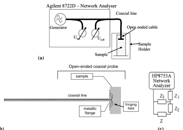
2.1. Low frequency (1 mHz - 10 MHz) dielectric spectroscopy measurements 47 2.2. High pressure (0.1-700 MPa) setup for dielectric spectroscopy measurements 52 2.3. Very high pressure (0.1 MPa - 3 GPa) setup for dielectric spectroscopy

measurements 54

2.4. High frequency dielectric measurements 55

3. Study of Relaxation Dynamics of Aqueous Systems at Low Temperature and High

Pressure: A) Mixtures of Water and Glycol Oligomers 63

3.1 Relaxation dynamics of water in propylene glycols oligomers 63

3.1.1 Experimental details 63

3.1.2 Effect of water concentration at ambient pressure 65 3.1.3 Quantitative analysis of dielectric spectra 69 3.1.4 Similarity of ν-process to secondary relaxation 71 3.1.5 Effect of high pressure on the parameters of the relaxation dynamics 72 a) Analysis of dynamics: T and P dependence of τα and τν relaxation times 72 b) Analysis of dynamics: effect of pressure on Tg and Tcross, on fragility and

on activation energies 79

c) Analysis of dielectric strength: evidence of local mechanism for water

relaxation 84 3.1.6 Effect of the number of repeating units of the oligomers on dynamics 87

3.1.7 Comparison of low (4%) and high (26%) water concentration mixtures

with PPG400 at elevated pressure 98

3.2 Dynamics of water mixed with ethylene glycol oligomers 107 3.3 Conductivity: the measure of translational diffusion of ions 113

3.4 Conclusions 116

4. Study of Relaxation Dynamics of Aqueous Systems at Low Temperature and High

Pressure: B) Mixtures of Water and Saccharides 119

4.1 Systematic study of dynamics of water in water-fructose mixtures at different

isobaric and isothermal conditions 120

4.1.1 Experimental details 120

4.1.2 Analysis of dielectric spectra in presence of dc conductivity 122 4.1.3 Effect of high pressure on the parameters of the relaxation dynamics 127 a) Analysis of dynamics: T and P dependence of τα and τν relaxation times 127 b) Analysis of dynamics: effect of pressure on Tg and Tcross and on

activation energies 132

4.2 Comparison with other mono-, di-, poly- saccharides: from aqueous mixtures to

hydrated bio-polymers 139

4.2.1 Aqueous mixtures of monosaccharides: similarities and differences in

dynamic behaviour 139

4.2.2 Aqueous mixtures of disaccharides: a general scenario for water-sugar

solutions 144 4.2.3 Conductivity: the measure of translational diffusion of ions 153

4.2.4 Mixtures of water in polysaccharides: the case of the bio-macromolecule

glycogen 156 4.3 Dynamics of water in hydrated and solvated proteins: the example of

lysozyme-glucose system 162

5. Overview of the Characteristics of Water (ν-) Relaxation in the Metastable

Amorphous State of Aqueous Systems 171

5.1 Relaxation time (τν) of mixed, confined and bulk water 171 5.2 Dielectric strength of the ν-relaxation: another evidence of the individual nature

of water relaxation 180

5.3 Relaxation shape of the ν-relaxation 181

Conclusions 187

References 191

List of publications and conference contributions 207

General Introduction

When a liquid upon cooling avoids crystallization, it enters the supercooled (metastable) state. If the temperature continues to decrease, the consequent increase of viscosity is reflected in the molecular mobility in such a way that the characteristic relaxation times of cooperative motions of molecules become of the same order of the longer experimentally accessible timescales. Further cooling finally transforms the highly viscous liquid into a glass, in which configurational transitions are frozen and only local motions are allowed.

It is well known that the mobility at a microscopic scale, the temperature and pressure conditions determine the macroscopic properties of the materials, which also depend strongly on their chemical structures. Macroscopic response of the material can be originated by very different microscopic motions. In the low molecular weight substances, for example, simple (local) movements can consist in rotations or in very limited translations of the whole molecule. On the other hand, complex movements require cooperative motions with neighbour molecules.

Moreover, it is interesting to note that materials with very different chemical structures exhibit molecular mobility with similar features. In the molten state, one of the characteristics of the equilibrium liquid is the high rate of molecular or segmental (in the case of polymeric chains) mobility, both translational and rotational mobility are present. This dynamical behaviour suffers drastic changes when the temperature decreases or pressure increases (i.e., increasing of density) and the liquid becomes an amorphous solid (glass).

The evolution from supercooled liquid to a glassy solid is called glass transition. However this phenomenon is a kinetic process, not a proper thermodynamic transition, produced by the impossibility of the material to reach the equilibrium state (within reasonable observation time) when the temperature decreases. In other words, the glassy state is an out-of-equilibrium state in which the material lacks any molecular order: the material in this sense continues to be a liquid, but the conformational mobility is mostly frozen [1]. As a consequence, the substance presents a mechanical behaviour similar to that of solid materials (it cannot flow, it sustains a shear force, etc.), while it keeps a disorder typical of liquids, i.e. without long-range order.

Far from being an exceptional situation, there are many materials that easily form a supercooled liquid and a glass, thus named as glass formers, such as polymers, sugars, and their mixtures with water. Also in ordinary life, it is common to find situations where the glassy state is crucial. The preservation of life under extremes of cold dehydration and the stabilization of labile biochemicals [2], the processing of foods [3-5], the improvement of bioavailability in pharmaceutical products [6, 7] are some of several examples in which the glassy state plays an important role.

The most abundant substance in our planet Earth is water, which is present in significant proportion in all living organisms, and without which life is impossible. Since pure bulk water easily crystallizes on cooling, its relaxation dynamics in the supercooled state cannot be deduced from various experiments without uncertainty and controversy including its glass transition temperature, Tg. Therefore, the study of water mixtures, which do not crystallize on cooling,

serves yet another purpose that is, to infer, from the observed relaxation dynamics of water in the mixtures at various concentrations, the properties of supercooled pure water in its inaccessible temperature range below about 235 K.

That is why the study of the molecular dynamics of glass-forming binary mixtures of water with other hydrophilic substances is very interesting not only for practical purposes but for fundamental understanding of the glass transition.

The reorientational dynamics of water molecules, thanks to their very strong molecular dipole, can be successfully studied by broadband dielectric spectroscopy. This technique, present in Physics Department laboratory of the University of Pisa, allows for a very wide dynamic range from 10 ps up to 1 ks and can be applied both at ambient and very high pressure.

The thesis is organized as follows: Chapter 1 will introduce the general topics and phenomenology of glassforming liquids. The experimental setup and practical procedures will be described in Chapter 2. Chapters 3 and 4 will present the main results of our study.

The effect of temperature and pressure on the structural and secondary relaxation in aqueous mixtures with glycol oligomers will be discussed in Chapter 3. In particular, the effect of water concentration and molecular weight of solute on dynamics will be reported.

Chapter 4 will presents the results from experiments where the solutes are saccharides (mono-, di- and polysaccharides). The possible application of the results concerning the dynamics of saccharide-water mixtures to bio-relevant systems will be also discussed in this Chapter.

In Chapter 5 we will contribute to the discussion about common features in aqueous systems such as water mixtures, confined water in nanoporous media and water present in the hydration layer at the protein surfaces. A schematic picture about the general mechanisms of the dynamics of bulk water will be also presented.

Chapter 1

Polarization, Dielectric Relaxation Spectroscopy and Glass Transition

The interaction between an electric field and matter can be studied by Dielectric Relaxation Spectroscopy (DRS) in a wide range of frequencies (10-6–1011 Hz). The variation of the dielectric constant with frequency and temperature is very useful for getting information about dipolar reorientational motions and electric conduction that arises from translational motions of charge carriers. With this information it is possible to infer about the molecular reorientational motions and even about the molecular structure and arrangement of the system.

Since 1927, when Debye established the relationship between the dielectric relaxation and the orientational motions of molecular dipoles [8], the technique of DRS has been gaining progressively interest within the scientific community.

As this work is based in its majority in results acquired with this technique, it is important to present the basic concepts of BDS and theory that supports it.

1.1 Polarization

Since matter is constituted by electric charges, when an electric field is applied, an interaction is produced, taking, at equilibrium, to an arrangement of the charges different from that with no applied field. If free charges are present in the material, that interaction, together to some friction mechanism, results into a charge carrier drift that originates the conduction phenomenon. On the other hand, if the material is a dielectric, such a long range movement is not possible (or only in a weak way); nevertheless, the electric field is able to induce a deformation in the charge distribution with respect to the equilibrium situation. This displacement, with low intensity, is at the origin of polarization.

The basis of the theory of electric polarization is the development of electric potential φ(P) into the elementary charge distributions (unipolar, dipolar, quadrupolar, … terms):

... 1 1 : 1 1 ) ( = − ⋅∇ + ∇∇ − ∇∇∇ + r r r r e m Q U_M P φ , (1.1)

where m, Q, U are dipole, quadrupole and octupole moments, respectively, e electric point charge, r radius vector.

In most of the systems moment of unipole is equal to zero (electrically neutral) and contributions to the polarization field due to the higher order dipole moments could be considered negligible. If so, the polarization P is defined as a vector quantity that expresses the magnitude and direction of the overall electric dipole moment per unit volume in the material:

∑

= _i

V p

P 1 , (1.2)

where i counts all dipole moments in the system, pi=qiri i.e. the product of charge times the

position vector. Molecules have a dipole moment if there is a mismatch between positive and negative electric charge average. It is important to define the concept of dipole moment: two charges q with opposite polarity, separated by distance d, can be characterized with the dipole moment p=qd. For any distribution of charges the dipole moment can be expressed by

∫

=

Vr e r d r

p ρ ( ) 3 [9].

At first approximation, in the following, we will consider that the overall electric potential related to the charge distribution in our systems can be expressed completely in terms of electric dipole moment. We will not consider any multipole expansions. Moreover, due to the low electric field that we applied (less than 105 V/m), non-linear effects can be neglected. Moreover, the systems we studied can be considered isotropic, a fact that will allow us to consider the polarization vector always parallel to electric field and to expressing permittivity as a scalar quantity and not as a tensor (unlike, for instance, the case of ferroelectric materials).

According to a very simplified approach, at microscopic level three main different mechanisms can induce polarization in a dielectric material when it is subjected to an electric field: electronic, atomic and orientational [10].

Electronic polarization: it happens when the electrons undergo a displacement with respect to the nucleus by the action of the electric field. Actually, the intensity of the electric field inside the atom (~1011 V⋅m-1_{) is higher than those applied in the experiments (less than 10}8 _V⋅m-1_{); so}

this difference induces usually a weak polarization. This dipole moment can be induced by the external applied electric field or by the interaction with other molecular dipoles.

Atomic polarization: It is the result of the modification in the relative positions of atomic nuclei inside the molecule or in an atomic network as a result of the application of the external field. It is typical, for instance, in ionic crystals. The timescale on which such a displacement occurs is the same of movements of internal degrees of freedom like bending, twisting or stretching of

Orientational polarization: Only appears in polar materials, i.e. those systems possessing a static molecular or ionic dipole moments, and it is a result of the preferential orientation of these permanent dipole moments in the direction of the applied electric field.

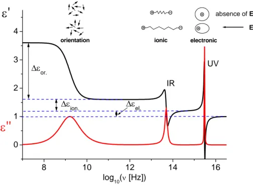
The times of response of the three types of polarization are very different in condensed matter: around 10-17 and 10-14 s for electronic, 10-13 to 10-12 s for atomic polarization, and between 103 and 10-12 s for orientational one (strongly dependent on temperature and material). Thus, the orientation of molecular dipoles is a relatively slow process in comparison with electronic transitions or molecular vibrations. Moreover, it does not mean that all molecules rearrange uniformly and instantly: It looks more like slight changes in their average orientations which proceed thermal fluctuations. The maximum polarization will be reached in material only when time after applying external electric field is sufficiently long to allow all molecules approach their equilibrium conditions. The physical quantity that describes how an electric field affects and is affected by a dielectric medium, and determines the ability of a material to polarize as a response to the field is called dielectric permittivity. The highest observable relative permittivity (or static dielectric constant), ε_S, in a material corresponds to the maximum value of its polarization (see fig. 1.1).

8 10 12 14 16 0 1 2 3 4 E absence of E electronic ionic orientation UV IR ∆ε_el. ∆ε ion. ∆ε_or.

ε

''

ε

'

log₁₀(ν [Hz])

Fig. 1.1. Mechanisms of polarization and frequency dependence of real and imaginary parts of dielectric permittivity.

On the other hand, if the polarisation is measured immediately after the field is applied (i.e. there is no time for dipole orientation to take place), then the observed instantaneous relative permittivity, denoted ε_∞, will be low and due to deformational (electronic and atomic) effects alone. Therefore, somewhere in between these extremes of timescale there must be a dispersion from a high to a low relative permittivity.

Figure 1.1 shows the frequency-dependent real and imaginary parts of dielectric permittivity upon application of an oscillating electric field with frequency ν, putting in evidence several facts: i) the frequency location of the different mechanisms involved in the polarization is quite distinct; ii) the intensity of each process is also quite different but the relative intensity could depend on the system; and iii) the width of the loss peaks is higher in orientational polarization due to the resistance that the medium puts up to the dipole’s motion [10] being far from an instantaneous response as the other two polarization mechanisms. Actually, the main difference between electronic and atomic polarization response on one side and orientational polarization response on the other side is the resonant behaviour of the first two, while the latter shows the characteristic non-resonant decay in the simplest case described by the Debye equation. Indeed, while in the first case the equation of motion for polarization is similar to that of a damped harmonic oscillator (with a quite high Q factor), the second case can be obtained for an overdamped oscillator, where the system returns or relaxes (exponentially decays) to equilibrium without oscillating. Actually the orientational motion of molecular dipoles in liquids is subjected to several frictional interactions with the surrounding medium.

1.2 Phenomenological description of dielectric measurement

In the thesis we will focus on the dielectric relaxation phenomena. The relaxation phenomena are very similar in the case of dielectric and viscoelastic response, as they occur, respectively, after application of electrical or mechanical stresses. The dielectric relaxation processes as well as mechanical can be described by means of general formalism, introducing a generalized force F and a generalized response x. In our case the generalized force or disturbance is the electric field

E, the associated generalized response is the polarization P of the system. The relation between

them is included in the linear-response theory (i.e. when the strength of the force is small, the response is proportional to that [10]). Thus the dependence of polarization P(t) on time

) ( )

(t ₀E t

P =χε , (1.3)

where the proportionality factor χ is called the dielectric susceptibility and 12 0 =8.854⋅10−

ε

F/m is universal constant, called permittivity of vacuum. If the electric field has very high intensity the proportionality no longer holds, and the polarization P can be expressed by a power series expansion of E:

∑

+ + = i i iE E E P χε₀ β 1 . (1.4)

From now and on only the linear approximation (Eq. (1.3)) will be considered, that is fully justified by the fact that the values of the electric field used in the experiment (less than 105 V/m) and the molecular permanent dipoles µ involved bring to values of energy (-µ⋅E) much smaller than the thermal energy (kBT ≈ 1/40 eV) or bond’s energy (10 eV) that correspond to the values

of electrical field of order E ≈ 109_-1011 _V/m.

From the definition of the vector of dielectric displacement the relation between susceptibility χ and dielectric permittivity ε follows:

) ( ) ( ) 1 ( ) ( ) ( ) (t E t P t ₀ E t ₀ E t D = + =ε +χ =ε ε , (1.5) χ ε = 1+ . (1.6)

It is important to note that ε depends on the material properties (structure and chemical composition) and physical parameters such as temperature and density. In the case of time-varying electric fields, if there is the dispersion phenomenon, the permittivity ε may depend on the frequency of the applied field. In fact, Eq. (1.3) implies an instantaneous response by the charge distribution of the system and it is true only for quasi-static case. On the contrary, when E changes in time faster than the characteristic time of the microscopic motion of the molecules, this latter will not be sufficiently rapid to build up the equilibrium polarization. On the other hand, it gives rise to a delayed response and a phase displacement between P and E, depending on the frequency of the field: this phenomenon is called dispersion. Following the principle of causality the value of the polarization assumed at time t depends on the values of the applied electric field at all previous moments:

∫

∞ − = _S t f t t t dt t) ( , ') ( ') ' ( ₀ E P ε χ . (1.7)

The function f(t,t') is called response function and it depends only on difference in times, ) ' ( ) ' , (t t f t t

timescale of the process (i.e. f(t,t')=δ(t−t'), the Dirac’s delta function), we obtain Eq. (1.3), with χS which is called static dielectric susceptibility, reflecting the value of susceptibility that is

obtained with time variation of the electric field much longer than the characteristic timescale of the system.

According to the formalism of linear response theory [11-14] Eq. (1.7) is nothing but the convolution integral between the response function (or Green function) f(t−t')and the electric field E. In other terms, the function f(t−t') is the response of the polarization of the system at time t' on the pulse electric field E =E0δ(t−t'). If the electric field of intensity E0 applied to the system is kept constant for some time and then suddenly removed at t =0, it can be represented with E₀⋅θ(−t), Heaviside step function. In that case, the produced electronic and atomic polarizations (also designed by induced polarization, Pin) disappear very fast (on a time

scale shorter of ps). In contrast, the orientational polarization falls down slowly (comparatively to those ones) with an exponential decay (as a first approximation, usually there is a distribution of such functions). The polarization response F(t) to a step function describing such a decay is called the relaxation function and related to f(t) by the following relation [11-13]:

dt t dF t

f( )=− ( ). (1.8)

After sufficiently long time after removal of the electric field the polarization of the system (and the relaxation function F(t) associated with it) vanishes: limit values assigned to the relaxation function are therefore F(t=0)=1 and F(t→∞)=0 [11-13] (see also fig. 1.2).

0 300 600 0 1 2 0 1 0 F(t) t f(t)

In other words, the evolution of the system towards its equilibrium after removal of the electric field is called the relaxation phenomenon. This lag in response is due to the internal friction of the material, and it can be related to viscosity η. For viscoelastic relaxation, in fact, according to the Maxwell model, the shear relaxation time is proportional to viscosity τ =η/G_∞, being G_∞ the infinite frequency shear modulus [15]. More is the viscosity of the medium, slower is the relaxation. Keeping this in mind, naturally arises the necessity to define a parameter that describes the polarization loss dynamics when the electric field is turned off. This parameter is the characteristic time, known also by relaxation time (required time to polarization decreases a factor 1/e from its initial value), and its average value can be measured by the integral of the relaxation function:

( )

∫

∞ = 0 dt t F τ . (1.9)

To analyse phenomena characterized by an arbitrary time dependence is useful to move the analysis of phenomena from the time domain to the frequency domain. This is possible due to the linearity of the response of the system: applying the Laplace transform to Eq. (1.7) with respect to iω (ω=2πν, angular frequency of the applied field), it is obtained from the relation of direct proportionality between transformed electric field and polarization which defines the complex dielectric susceptibility χ(ω):

) ( ) ( ) (ω ε₀χ ω E ω P = . (1.10)

The χ(ω) is, in contrast to the static susceptibility, the Laplace transform of the response function f(t) of the system: dt e t f i i t S

∫

+∞ − = − = 0 ) ( ) ( '' ) ( ' ) (ω χ ω χ ω χ ω χ . (1.11)

Substituting Eq. (1.8) in Eq. (1.11) and partially integrating one can obtain the relation between the relaxation function F(t) and the complex dielectric susceptibility χ(ω):

⎟⎟ ⎠ ⎞ ⎜⎜ ⎝ ⎛ − = _i +∞

∫

_{F t e}−i t_dt S 0 ) ( 1 ) (ω χ ω ω χ . (1.12)

On the basis of Eqs. (1.5) and (1.6) the complex dielectric permittivity can be defined in the frequency domain, ε(ω)=ε'(ω)−iε ''(ω): ) ( 1 ) (ω χ ω ε = + . (1.13)

The real part of susceptibility χ' and the permittivity ε' is the polarization component (in phase with applied electric field) which is related to a measure of the oriented molecules with electric field and of the fraction of the stored electromagnetic energy per period. On the other hand, the imaginary part of two variables is related to dissipated energy during the process (out-of-phase component) [11-13]. It can be also calculated the power L dissipated by the system in a period by the time averaging of the expression E⋅(dP/dt) [11-13] and the result, for a harmonic electric field with amplitude E0 and frequency ω, is L=πE₀2ωε₀χ ''(ω). For this reason the imaginary

part of permittivity, ε", is also called dielectric loss factor and the ratio tan(δ)=ε ''(ω)/ε'(ω), corresponding to the ratio between dissipated and stored energy for the period of oscillation, it is called the dielectric loss factor or dissipation factor [16]. It contains no more information than

) ( ' ω

ε and ε ''(ω), but this ratio can be obtained directly from complex capacitance independently of the capacitor geometry. This is particularly important if the capacitor geometry is not well defined. Furthermore, tan(δ) is used as a measure of the sensitivity of dielectric equipment. Recently, dielectric equipment able to measure tan(δ) ≈ 10-5 has become available [17].

Dielectric relaxation spectroscopy apparatuses are precisely based in the measure of the loss of polarization (i.e. dielectric relaxation) after the step removal of an external electric field at a certain temperature or pressure. The way as these dipoles relax will be rationalized in terms of molecular mobility existing in the system. Alternatively, a field sinusoidally changing with time is applied and the gain and phase displacement of the polarization response at different frequencies are acquired, taking to the so-called dielectric spectra.

When a relaxation happens, this can be detected either as a peak in the imaginary part or as an inflexion in the curve of the decrease of real part of susceptibility (and thus permittivity). That means that the two components are not independent: in fact, for a system that is linear, causal and stationary (i.e. independent of the choice of the time axis origin), as previously hypothesized, the real and imaginary parts are connected by the Kramers-Kronig (KK) dispersion relations [10, 18, 19]:

∫

∞ − = 0 2 2 ) ( '' 2 ) ( ' ξ ω ξ ξ ξχ π ω χ P d ;

∫

∞ − − = 0 2 2 ) ( ' 2 ) ( '' ξ ω ξ ξ ξχ ω π ω χ P d . (1.14)

The letter P indicates that it is needed to calculate the main part of the integrals [14].

∫

∞ ∞ = ₋ − 0 2 2 ) ( '' 2 ) ( ' ξ ω ξ ξ ξε π ε ω ε P d ;

∫

∞ ∞ − − − = 0 2 2 ) ( ' 2 ) ( '' ξ ω ξ ε ξ ε ω π ω ε P d . (1.15)

For the derivation of the Kramers-Kronig relations it has been used that: 0 = −

∫

∞ ∞ − ξ ω ξ d P . (1.16)

Eqs. (1.15) give the opportunity to obtain one part of the complex dielectric permittivity (real or imaginary) if another part (imaginary or real) is known from experiment. Actually, two singularities occur in Eqs. (1.15) when it is not possible to obtain unequivocally real part from imaginary and vice versa. First, when the real part of dielectric permittivity is constant with ω (in practice equal to ε_∞ or ε_S) Eq. (1.15 right) leads to Eq. (1.16), i.e. to 0. Second, when the imaginary part of dielectric permittivity is proportional to 1/ω (it could be in the case of dc conductivity term in dielectric spectra) Eq. (1.15 left) leads again to Eq. (1.16).

It is important to note that if only real part of the complex dielectric permittivity, ε'(ω), is known from experiment it is not possible to obtain dc conductivity using Kramers-Kronig relations (a true conductivity term proportional to 1/ω in the ε ''(ω) spectra gives no contribution to the real part), and on the other hand, if only ε ''(ω) is known from experiment it is not possible to obtain the value of ε . It is so clear the importance to analyse simultaneously both _∞ real and imaginary part of permittivity.

1.3 Debye model and related empirical models

Debye in 1929 presented a work on dielectric properties of polar liquids [20] where he proposed that for a dipolar system in non-equilibrium, relaxation takes place with a rate that increases linearly with the distance from equilibrium.

This statement can be written by a first order differential equation such as:

D t P dt t dP τ ) ( ) ( − = , (1.17)

where τ is a characteristic relaxation time. Three assumptions were made: i) negligible _D interactions between dipoles, ii) only one type of process brings to the equilibrium (i.e. either a transition above a potential barrier either a rotation with friction) and iii) all the dipoles can be considered equivalents, that is, all of them relax in average with only one characteristic time.

Eq. (1.17) leads to an exponential decay for the correlation decay function Φ : (t) ⎥ ⎦ ⎤ ⎢ ⎣ ⎡ − = Φ D t t τ exp ) ( . (1.18)

The relation for the complex permittivity in the frequency domain can be obtained as [21]: ⎟⎟ ⎠ ⎞ ⎜⎜ ⎝ ⎛ + − − ⎟⎟ ⎠ ⎞ ⎜⎜ ⎝ ⎛ + − + = + − + = ′′ − ′ = ∞ ∞ ∞ ∞ ∞ 2 0 2 0 0 * ) ( 1 ) ( ) ( 1 1 ) ( ) ( ωτ ωτ ε ε ωτ ε ε ε ωτ ε ε ε ω ε ω ε ε i i i . (1.19)

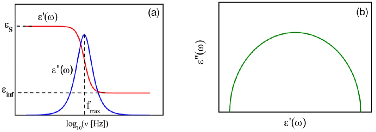
This is the well-known Debye dispersion equation. Plots of the characteristic shapes of real and imaginary parts of _ε* _{against ν =ω/2π (ν is the frequency of the outer electrical field) for this}

model are shown in fig. 1.3 (a). The imaginary part exhibits a symmetric peak whose maximum value occurs at ω_maxτ =1 and has an amplitude of ε_max′′ =(ε_S −ε_∞)/2. The breadth of the peak at half the height covers 1.14 decades of frequency [11].

The real part shows dispersion falling from ε_S to ε with increasing frequency. The most _∞ probable relaxation time of the process, τ , is defined as the inverse of ω_max (τ =1/2πf_max). The Debye response behaviour is observed in very few materials among which are organic liquids (acids and monohydroxy alcohols) [22-24] and liquid crystals [25]. For more complex systems as it is the case of supercooled liquid and polymers, this model fails to represent experimental data since most of the Debye assumptions are not satisfied: in fact molecular dipoles strongly interact, multiple processes bring to relaxation (with a distribution of activation barriers and of relaxation times), and not all the dipoles are equivalent, since, even in homogeneous systems, a dynamic heterogeneity sets up at molecular scale.

f_max ε_inf ε S ε"(ω) (a) ε'(ω) log₁₀(ν [Hz]) (b) ε

''(

ω

)

ε

'(

ω

)

Treating dielectric data, it is sometimes useful to construct the plot of imaginary part vs. real part of permittivity, known by Cole-Cole plot. In this representation, the Debye model corresponds to a symmetric semicircle arc (see fig. 1.3(b)).

Usually the measured dielectric functions in most of systems are much broader than predicted by the Debye function. Moreover, in many cases the dielectric function is asymmetric, i.e. that means that the short time (high frequency) behaviour is more pronounced than the long time (low frequency) one. This is called non-Debye or sometimes non-ideal dielectric relaxation behaviour. To take into account such phenomena Wagner proposed to use a continuous distribution of relaxation times [26]:

( )

∫

∞ = ∞ ∞ + = − − 0 ln 1 ) (ln τ τ ωτ τ ε ε ε ω ε d i G S , (1.20)

with logarithmic distribution function:

1 ln ) (ln 0 =

∫

+∞ = τ τ τ d G . (1.21)

The corresponding expression for the response function is:

( )

_∫

∞

(

)

= − = 0 ln ) (ln exp τ τ τ τ G d t t F . (1.22)

In the literature, much attention has been paid to the problem of obtaining information about distribution function from experimental results, although not in all cases the distribution function has a direct meaning. Mostly, the experimental results are represented as values of ε'

( )

ω and

( )

ω

ε '' at a number of frequencies. And approximate relations between G(lnτ) and frequency dependence of ε'

( )

ω and ε ''

( )

ω at ω =1/τ can be obtained only if the width of the distribution function )G(lnτ is large with respect to that of the graph for ε ''

( )

ω against lnω for a single relaxation time [10].

In many cases the non-Debye relaxation behaviour in the time domain is empirically described by the Kohlrausch-Williams-Watts (KWW) function [27, 28] (KWW-function) also named “stretched exponential function”, that is:

⎥ ⎥ ⎦ ⎤ ⎢ ⎢ ⎣ ⎡ ⎟⎟ ⎠ ⎞ ⎜⎜ ⎝ ⎛ − = Φ KWW KWW t β τ τ) exp ( . (1.23)

The stretching parameter β_KWW (0 <β_KWW≤ 1) leads to an asymmetric broadening of Φ(τ) at short times compared with exponential decay (β_KWW =1, the case of simple Debye relaxation

behaviour). τ_KWW is the related relaxation time. KWW function has not analytic Fourier transform to the frequency domain. In the frequency domain the relaxation data are often described by the empirical function of Havriliak and Negami (HN) [29] which reads

HN HN HN HN _iωτ α β ε ε ω ε ) ) ( 1 ( ) ( ₁ * − ∞ ₊ ∆ + = . (1.24)

The fractional shape parameters (1−α_HN) and β_HN (0<(1−α_HN); 1(1−α_HN)β_HN ≤ ) describe symmetric and asymmetric broadening of the complex dielectric function. Moreover (1−α_HN) and β_HN are related to the limiting behaviour of the complex dielectric function at low and high frequencies, that are asymptotically described by power laws:

) ( 0 ε ω ε − ′ ∼_ωm_{; ε′′∼ω}m _{for ω<<} HN τ / 1 with m=(1−α_HN), (1.25) ∞ − ′ ω ε ε ( ) ∼_ω−n_{; ε′′∼ω}−n _{for ω>>} HN τ / 1 with n=(1−α_HN)β_HN. (1.26) Some examples of the behaviour described by Havriliak-Negami function are shown in fig. 1.4.

2 4 6 8 10 12 0 2 4 6 8 _(a) α = 0 β = 1 α = 0.6 β = 1 α = 0 β = 0.4 ε '( ω ), ε "( ω ) log₁₀(ν [Hz]) 2 3 4 5 6 7 8 0 1 2 3 4 α_α = 0 _{= 0.6} β_β = 1 _{= 1} (b) α = 0 β = 0.4 ε ''( ω ) ε'(ω)

Fig. 1.4. (a) Frequency dependence of the real, ε′, and imaginary, ε′′, parts of permittivity. (b) Imaginary part vs. real part of ε*. Continuous lines show the Debye function case, dotted lines show the

HN function with α_HN=0.6 and β_HN=1 (symmetric case) and dashed lines show the HN function with

HN

α =0 and β_HN=0.4 (asymmetric case).

The frequency of maximum ε", fmax, can be analytically calculated from the HN fitting

parameters by:

(

)

. ) 1 ( 2 ) 1 ( sin ) 1 ( 2 ) 1 ( sin 2 1 1/(1 ) 1/(1 ) max ⎟⎟ ⎠ ⎞ ⎜⎜ ⎝ ⎛ + − ⎟⎟ ⎠ ⎞ ⎜⎜ ⎝ ⎛ + − = − − − − β β α π β α π πτ α α HN f (1.27)

The most significant parameter of a single relaxation process is the characteristic relaxation time τ, which is also the average time, that is the area below the peak curve of the different relaxation spectra. In the case of a distribution of relaxation times, a significant value is which represents the most probable time. It can be easily obtained from Eq. (1.27) as τ =

(

2π⋅ f_max

)

−1, which is usually preferred to τHN since it is a model-independent parameter.

It is important to note that Eqs. (1.19) and (1.24) are theoretically compatible with Kramers-Kronig relations (Eqs. (1.15) and (1.16)).

The quantity ∆ε =

(

ε_S −ε_∞

)

in Eq. (1.24) is named dielectric relaxation strength and it is a measure of the orientational contribution to polarization. It can be obtained from the difference between low and high frequency of the real part of permittivity or from the area below the imaginary part versus logarithm of frequency of the loss peak (see fig. 1.1). In a molecular liquid dielectric strength can be described by the equation [30]:

2 3 4π _µ ε _{K A} B N Fg T k C = ∆ , (1.28)

where NA is the Avogadro number, kB the Boltzmann constant, µ is the molecular dipole

moment, C is the number of effective dipoles per unit volume, F is the local field correction, gK

is the Kirkwood correlation factor which gives the local static angular correlations between the dipoles.

Eq. (1.28) was generalized on the basis of Debye formula [30] by Onsager [31] and later by Kirkwood [32-34] and Fröhlich [21]. Onsager obtained it for polar molecules by the theory of the reaction field [31] which considers the enhancement of the permanent dipole moment of a molecule µ by the polarization of the environment. In practice Onsager equation fails for polar associating liquids because interactions of neighbouring molecules are not considered in the derivation of the equation. Therefore, Kirkwood [32-34] and Fröhlich [21] introduced the correlation factor gK to the model of the dipole interaction. In the first approach to calculate

Kirkwood correlation factor, only the nearest neighbours of a selected test dipole are considered and gK can be approximated by:

( )

T 1 z cosψ

g_K = + , (1.29)

where z is the coordination number and ψ is the angle between the test dipole and a neighbour [9, 30]. In practice gK is very difficult, if not impossible, to obtain on a molecular basis, thus Eq.

correlation factor gK from measured ∆ε. Usually all the quantities involved have a very weak T

dependence, excepting gK that has a temperature dependence that can be approximated as a first

order polynomial: therefore the overall temperature behaviour can be represented by a first order polynomial in 1/T, so if the number of effective dipoles per unit volume C is nearly constant, ∆ε usually decreases with increasing temperature for a structural α-process. If the number of effective dipoles on the other hand increases on increasing temperature, as it occurs for secondary (local) relaxation processes (that usually have to overcome an activation barrier), ∆ε is found to increase with temperature.

1.4 Molecular dynamics and the glass transition problem

1.4.1 Molecular dynamics and macroscopic response

Why is the knowledge of the macroscopic electric response important for understanding the molecular dynamics? Because the linear response theory relates the macroscopic response function to microscopic dynamics, i.e. to the spontaneous fluctuations of an observable due to molecular motions [13, 35, 36]. Let’s consider the stochastic fluctuations of the microscopic variable x(t) (for instance x(t) = p(t) microscopic polarization). We can suppose that the expectation value <x(t)>, i.e. the average on the ensemble of all the possible values of x(t) in the system, is constant with time (stationary process) and it is equal with the time average (ergodic process). Assuming, for making it simple, that <x(t)>=0 (that can be always obtained by subtracting the average value), the autocorrelation function x(t) can be defined as:

( )

t = x

( ) (

t′ x t′+t

)

ϕ . (1.30)

This function describes the correlation degree of the variable x at the instant t′+t with the same variable at time t′; when the autocorrelation function is zero it means that events differing more than time t are statistically not related. The knowledge of φ(t) provides important information about the microscopic dynamics of the system and it allows to directly check theoretical predictions on molecular dynamics, so important to define unsolved problems as that of the glass transition. Some spectroscopic techniques allow to acquire, directly or less directly, φ(t). Concerning the spontaneous fluctuations of the microscopic polarization p(t) there are some methods based on dielectric noise analysis [37, 38] that allow to obtain φ(t), with very strong

that can be obtained from a dielectric relaxation experiment (by means of permittivity). Conventional dielectric spectroscopy provides information on the autocorrelation function of the macroscopic polarization. In fact, according to Kubo relation [13], the relaxation function Φ(t) and the autocorrelation function are related as:

( )

1 (0) ( ) 1 p(0) p(t) p(0) p (t) (t) (t) T k t P P T k t i j j i i i B B Ψ + = ⎥ ⎦ ⎤ ⎢ ⎣ ⎡ ⋅ + ⋅ = ⋅ = Φ

∑

≠ φ r r r r r r , (1.31) where T is the temperature in Kelvin and kB is the Boltzmann constant, Pr is overall electric

dipole moment per unit volume defined by Eq. (1.2), pr is microscopic dipole moment, φ(t) is the microscopic autocorrelation function, Ψ is the cross-correlation term. Therefore, only (t) when the cross-correlation term is negligible, i.e. when microscopic dipoles are non-interacting, dielectric spectroscopy can give information on the microscopic dynamics. Unfortunately, this case occurs very rarely, for instance in very diluted dipolar solutions.

Moreover, it is possible to relate the autocorrelation function Φ(t) to the power spectrum I(ω) of the fluctuations of P(t) and the latter to the imaginary part of the susceptibility, using the Wiener-Kintchine theorem and the fluctuation-dissipation theorem [13, 36]:

( )

( )

( )

∫

+∞ ∞ − − _{= =} ′′ Φ ω ω χ ω π t e ωdt I kBT t i ₂ 2 1 . (1.32)

Thanks to the above mentioned relations, we can affirm that the data obtained in relaxation experiments in a system with linear response provide information on the fluctuation dynamics of the examined system. Moreover, due to this achievement, it is equivalent to acquire data in time domain (through the response or relaxation function) or in frequency domain (through susceptibility to permittivity). If the microscopic polarization p(t) can be associated to reorientational motions of the molecular dipoles, dielectric spectroscopy experiments allow the direct study of microscopic molecular dynamics.

1.4.2 Slow Dynamics and Glass Transition

The motions of molecules constituting a liquid are known to slow down when the temperature is decreased or the pressure (or density) is increased. Eventually, if the liquid can be supercooled below its melting point or compressed beyond the melting curve without forming a crystal and kept in that metastable state also to much lower temperature or higher pressure, the dynamics of liquid can become so slow that eventually the molecules cannot attain their dynamic equilibrium

configurations on the time scale of observation, and the system becomes structurally arrested, with its structure similar to that of a liquid (i.e. without long range order). The amorphous solid so obtained is called glass.

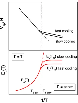
This falling out of equilibrium occurs across a narrow transformation temperature or pressure range where the characteristic molecular relaxation time becomes of the order of 102 s, and the rate of change of volume or enthalpy with respect to temperature decreases abruptly to a value comparable to that of a crystalline solid [39]. Figure 1.5 illustrates the temperature dependence of a liquid's specific volume (or enthalpy) at constant pressure. The glass transition is defined by the change of slope in the temperature dependence of the considered quantity (thermodynamic definition). In this figure, a slow cooling rate will bring the system out of equilibrium later and at a lower glass transition temperature TgSlow, corresponding to a smaller specific volume or

enthalpy, whereas a faster cooling rate will lead to a glass transition at a higher TgFast with a

bigger specific volume or enthalpy. So, Tg increases with cooling rate.

H

Fig. 1.5. Temperature dependence of the specific volume (or enthalpy) of a glass former. Tm is the melting temperature, Tg is defined as the temperature at which the liquid and the glass V(T) curves intersect. Tg depends on cooling rate which is faster for “glass 1” (reproduced from ref. [40]).

The glass transition temperature is not associated to the discontinuity of any thermodynamic variable but to the temperature range where the transition to the out-of-eqilibrium amorphous solid state occurs. The common definition of T in terms of thermodynamic properties is reported

above. According to dynamic properties, Tg is the temperature at which the shear viscosity

reaches 1013 poise or the structural relaxation time (usually proportional to viscosity) reaches 100 s (as was mentioned above, more viscous is system slower is the relaxation process, i.e. the relaxation time is proportional to the viscosity of the material).

Thus the glass transition or vitrification is nothing but the manifestation of the dramatic slowing down of kinetic processes, such as diffusion, viscous flow and molecular reorientations. Such a phenomenon is very general and it has been found in organic, inorganic, metallic, polymeric, colloidal, and biomolecular materials. It is not typical of some material: usually molecular liquids with complex chemical structure are more prone to form glasses, as well as some disordered systems like atactic polymeric melts, but recently vitrification was shown in simulation also for very simple systems like argon [41]. The most important variable seems to be the cooling rate: if one is able to quench a liquid fast enough, a glass will be obtained.

In summary, as a phenomenon, it is recognized that glass transition is the arrest of the structure from reaching equilibrium, and is well understood simply from kinetics consideration. Its main cause is the slow structural relaxation (see section 1.5.1). A fundamental understanding of glass transition requires the knowledge of the dynamics of the structural relaxation and the identification of the factors that make τα to slow down drastically with decreasing temperature or

increasing pressure. Surprisingly, in spite of the long history of the phenomenon and technological significance of glass, there is still no universally accepted view on the dynamics of the structural relaxation, so that this is one of the unsolved question of condensed matter physics (see [42, 43]). There is no consensus on the factors governing the dramatic slowing down of the structural relaxation and related kinetic processes, such as viscous flow and diffusion. Development of a microscopic and quantitatively accurate theory of the glass transition that is generally applicable to real materials, has become even more challenging with the improvement of experimental techniques and the introduction of new ones. These advances have led to the discovery of an increasing number of general properties of the dynamics of glass-forming materials spanning the range from picoseconds to years. In fact, accurate spectroscopy techniques show that not only the slow structural relaxation is important for glass transition, but also other faster processes. An accurate theory should take into account all these phenomena spanning the whole dynamic range.

Glass transition is currently still the subject of active research with many participants, and the theme of many international scientific conferences [44-46]. Its study is no longer limited to the

few traditional areas concerning the amorphous structural materials (silicate and polymer glasses), but has branched out to electronics and opto-electronics, metallurgy, geoscience, materials for energy source applications, and others. The study of glass transition has recently received a boost from activities in nanoscience and nanotechnology, where the changes found in the dynamics of the structural relaxation and glass transition temperature present new challenges [47-50]. Other recent fields where glass transition is of great interest are biology, pharmacy, medicine and food industry: protein dynamics seem to resemble that of very complex glass-forming polymers [51]; drugs have been found to be more soluble (so more bio-available) in their amorphous (glassy) state than in their crystalline [7]; aqueous mixtures with glycols and sugars are commonly used for the food storage, conservation and for the cryo-preservation of the biological systems [52, 53].

1.5 Relaxation phenomena in glassy systems

In physics, the relaxation phenomenon means the return of the macroscopic system to the thermodynamic equilibrium after removal of an external perturbation. For example, in our case a system can be perturbed from its equilibrium state by the electric field, whereby the energy from the external source can be dissipated in the system in characteristic time-regions which are determined by the molecular structure of the glassy system. These are the relaxation processes in which configurational rearrangement of atomic or molecular constituents of the glass is induced by the external stress (electric field) which must be small compared with, for example, the electrical forces acting between the constituent particles. These relaxation processes may be monitored by different ways, some of which determine the volume or enthalpy of the system, while others the permittivity or the optical density at frequencies characteristic of specific subunits of the glass structure are determined. Moreover, the characteristic time scales of the relaxations are of particular interest in material science because, in contrast with frequencies of resonant phenomena, they are highly temperature-dependent, varying over 13-15 orders of magnitude between the glass temperature and the normal melting temperature. Generally, relaxation processes are named successively by the order of appearance at fixed frequency on cooling the system, by the Greek letters α, β, γ, δ and can be classified according to their time scale in the following order:

(i) At the longest time scale structural changes are allowed by collective, cooperative motions that involve the rearrangement of groups of molecules or the segmental motions of polymer chains. In this case the dynamics is controlled by the α-relaxation, named also the structural relaxation which is the main universal dynamical process related to the glass transition (see fig. 1.6) and describes the situation near Tg with the α-peak situated at a rather low frequency. On

increasing temperature it will rapidly shift to higher frequencies.

(ii) At shorter times, the molecular motions are cooperative. These faster and non-cooperative processes are present as well in the viscous liquid state as in the glassy state and are generally more localized than the cooperative α-process. Their behaviour in the glassy state is purely activated. They are usually called secondary or β-relaxation processes. Because of the disordered structure of the glass, a large distribution of the barrier energy can be present. In some systems with several degrees of freedom, several secondary relaxations can be present (they are labelled as β-, γ-, δ-, etc.).

(iii) At some THz a second loss peak shows up, which can be identified with the so called boson peak (see fig. 1.6) known from neutron and light scattering [9]. The boson peak is a universal feature of a glass system and corresponds to a low frequency excess in the vibrational density of states.

Fig. 1.6. Schematic view of the dielectric relaxation loss spectra in glass-forming systems for one temperature. The α-relaxation related to the dynamic glass transition, the excess wing, the fast β-process, the boson peak and infrared bands (intramolecular modes) at the highest frequencies are shown (reproduced from ref. [54]).

In the following sections, we will introduce and discuss the main features of the structural α-relaxation and secondary β-α-relaxation.

1.5.1 The structural relaxation

The central and most important dynamical phenomenon in glass-forming systems is the α -relaxation. It is undoubted that every glass shows this type of dynamics and certain characteristics are always observed [55]. On decreasing temperature T or increasing pressure P, the structural relaxation time τα of supercooled liquids becomes increasingly long.

The most prominent features of the α-relaxation resulting from structural disorder are non-exponential relaxation patterns and a non-Arrhenius temperature dependence of the characteristic timescale [41, 56].

a) Non-exponentiality and dynamic heterogeneity: As was mentioned before (see section 1.3),

differently to a simple Debye relaxation phenomenon in which the correlation function is described by a simple exponential function, the structural relaxation appears more slowly and it can be described by the empirical stretched exponential [10] or the Kohlrausch-Williams-Watts type decay [27, 57] for a very broad class of materials [27, 41]. The deviation from the simple to the stretched exponential function describing the time dependence of the relaxation functions when a liquid is supercooled should be related to two reasons:

- The “cage effect” which is already present in the normal liquid but should become more pronounced on increasing density, i.e. when temperature decreases or pressure increases. “Thus, the long time dependence of the relaxation functions should have a larger temperature dependence on approaching the glass transition than the short time dependence and the motion will be more and more cooperative as the molecular packing increases, whereas the latter is related to ‘in cage’ motions and is thus less affected by the freezing of the cages. This difference explains the stretching as well as the increased temperature dependence of the relaxation times, which are dominated by the long time dependence” [58].

- Dynamic heterogeneity which is now recognized as a fundamental feature of the slow dynamics of supercooled fluids and glasses in condensed matter. Heterogeneity regarding the dynamics refers to the picture in which fast and slow relaxing modes exist [56, 58-63]. There is a long

for a comprehensive review on heterogeneity and dynamics see the papers by Prof. Sillescu [58] and Prof. Richert [56]. The sizes of these domains, which are dynamically distinct, are assumed to be of the order of several nm [59-62]. Taking a snapshot of a glass-forming system, in the same environment some molecules are characterized by fast motions, while others are much slower, acting as cages for the faster. This picture is dynamic, in the sense that, few moments later (usually on the time scale of the structural relaxation τ_α) due to the mutual interactions, the fast molecules could become slow and vice versa. Fast and slow molecules are usually clustered in domains. One could be tempted to explain the stretched exponentiality character of the relaxation in glass-forming systems, simply assuming that, in each spatial domain, relaxation occurs exponentially but with a different relaxation time in each domain: averaging over the ensembles, this should lead to a distribution of relaxation times. Following this idea, Ediger et. al. [63] proposed a spatially heterogeneous model of translational and rotational diffusion in supercooled liquids, i.e. the different temperature behaviour of the two quantities reported in the region Tg<T<1.2Tg. In fact translational diffusion was found less temperature dependent than the

rotational one. According to Ediger the decoupling could be due to the different prominences that fast and slow motions have on translational and rotational diffusion, respectively: therefore, if spatial heterogeneity reflects into a given distribution of relaxation times for the α-relaxation, wider is the distribution stronger is the decoupling between translational and rotational diffusion. On the contrary, some experimental evidences for organic glass-formers (for instance ααβ-tris-naphthylbenzene (TNB) [64, 65], showed that the width of the relaxation peak (and so the distribution of relaxation times) was temperature independent over a broad temperature range, while in the same temperature range a decoupling between translational and rotational diffusion was found. An alternative explanation was proposed by the coupling model (CM) (see section 1.6) according to which decoupling of translational and rotational diffusion in glass-forming liquids is a special case of a more general phenomenon, i.e. that different dynamic observables weigh the many-body relaxation differently and have different coupling parameters n (i.e. different degrees of intermolecular cooperativity) that enter into the stretch exponents βKWW of

their Kohlrausch correlation functions but also in the temperature dependent considered observable [66, 67].

Concerning the homogeneous scenario, among the models proposed in recent years, the one that received the most attention is the Mode Coupling Theory (MCT) developed by Götze and Sjögren [68]. This theory gives one of the interpretation of the complex microscopic dynamics of

simple supercooled liquids. The MCT predicts and explains a wide range of phenomena relating to the glass transition with a small number of basic assumptions and concepts borrowed from the dynamics of simple liquids. Despite of the validity and applicability of this theory it is still a matter of debate [69, 70]. Some results of this model are certainly interesting and shown below along with the main features of the MCT model.

The Mode Coupling Theory directly calculates the autocorrelation function of the density fluctuations of a liquid φ(t), through which one can go back to the relaxation function (see § 1.2) and monitor the dynamics of the system. The function φ(t) describes the correlation between the positions of the molecules, i.e. it measures the probability of finding a molecule in certain position x at time t (initial conditions: x = 0 at time t = 0). According to the MCT for φ(t) the following equation is valid [68-70]:

0 ' ' ) ' ( ) ' ( ) ( ) ( ) ( 0 2 0 2 2 = − + + Ω +

∫

dt dt t d t t m dt t d t dt t d φ _{φ γ} φ t φ (1.33)

Eq. (1.33) is generalized equation of motion (Langevin equation) of an overdamped harmonic oscillator: the elastic collisions between the molecules lead to the fluctuations with frequency

0

Ω , related to phonon frequency, and to a dissipative term (γ is the friction coefficient). The fourth term of Eq. (1.33) is called memory term since it describes the effects happened at time t' before the density fluctuations occurred (t'<t) and represents the feedback exerted on the molecule by the surrounding molecules. Since the memory term m(t) depends on the product of the density correlation functions, obtained solution of Eq. (1.33) is self-consistent. At low density (i.e. high temperature) the collisions are statistically independent and the uncorrelated ones contribute only to the friction term γ and the memory term disappears. The result, when the friction term overwhelms the inertial one (i.e. the second derivative), is the same as in Debye model, and so the correlation function is an exponential decay. On increasing density collisions are more correlated and a molecule, at shorter times, becomes caged by the surrounding particles. Increase of the damping motion is represented by Eq. (1.33) when the memory term increases. At longer times the molecule can escape from the fluctuated "cage" and further diffuse. The corresponding friction coefficient apparently relates to the memory term. According to this view, the relaxation is developed in two stages: first the vibrational component relaxes (related to the motion of the molecule inside the "cage") and then slower motions related to the decay of the "cage" effect and to the diffusion.