Computing multirobot paths for joint measurement gathering

(1)

POLITECNICO DI MILANO

Master of Science in Computer Science and Engineering Dipartimento di Elettronica, Informazione e Bioingegneria

Computing Multirobot Paths

for Joint Measurements Gathering

Supervisor: Prof. Francesco Amigoni Co-supervisor: Ing. Jacopo Banfi Co-supervisor: Ing. Alessandro Riva

Carlo Leone Fanton, 780525

(2)

(3)

(4)

(5)

Abstract

Multirobot systems represent a major sub-field of mobile robotics whose challenges have received a growing attention from researchers in the last few years. Specifically, the problem of performing joint measurements recurs in many robotic applications, like in constructing communication maps from signal strength samples gathered on the field, and in localization and posi-tioning systems.

In this work, we consider an environment represented by a metric graph where a team of robots has to perform a given pre-specified set of joint measurements, which represent the locations where information gathering is needed. The aim of this thesis is to solve one fundamental problem emerg-ing from this scenario: seekemerg-ing joint paths for the robots to perform all the required measurements at minimum cost.

We prove that the problem of jointly performing measurements from given vertices is NP-hard when either the total traveled distance or the task completion time has to be minimized. Given the difficulty of finding optimal paths in an efficient way, we propose a greedy randomized approach able to cope with both the optimization objectives. Extensive experiments show that our algorithms perform well in practice, also when compared to an ad hoc method taken from the literature.

(6)

(7)

Sommario

I sistemi multirobot rappresentano un’importante area di ricerca nel campo della robotica, e stanno ricevendo sempre maggiore attenzione dai ricerca-tori. In particolare, il problema di eseguire misurazioni congiunte ricorre in molte applicazioni, come nella costruzione di mappe di comunicazione derivanti dal rilevamento di campioni di potenza del segnale, oppure nei sis-temi di localizzazione e posizionamento.

In questo lavoro, consideriamo un ambiente rappresentato da un grafo metrico in cui una squadra di robot deve eseguire un insieme pre-specificato di misurazioni congiunte, rappresentate dai punti fra i quali `e richiesta l’acquisizione di informazioni. Lo scopo di questa tesi `e risolvere uno dei problemi fondamentali che emergono da questo scenario: trovare percorsi congiunti per permettere ai robot di eseguire le misurazioni richieste a costo minimo.

Proviamo che il problema di eseguire congiuntamente misurazioni su insiemi di vertici dati `e NP-difficile quando dobbiamo minimizzare il totale della distanza percorsa oppure il tempo di completamento. Data la difficolt`a di trovare percorsi ottimali in maniera efficiente, proponiamo un approccio greedy randomizzato capace di far fronte alla minimizzazione di entrambi gli obiettivi. Numerosi esperimenti dimostrano che i nostri algoritmi hanno buone prestazioni, anche quando confrontati con metodi ad hoc proposti in letteratura.

(8)

(9)

Ringraziamenti

Trovare le parole giuste per ringraziare tutte le persone con cui ho la fortuna di condividere la mia vita è più difficile che scrivere lo script Python su cui ho lavorato per mesi, ma ci proverò.

In primo luogo grazie al Professor Amigoni; il suo aiuto preciso, costante e sempre attento mi ha permesso di raggiungere questo importante tra-guardo. Grazie a Jacopo, presto Dott. Banfi, per il supporto e per i fon-damentali consigli che mi ha dato nella stesura di questo elaborato: sarai un super PhD iper ultra swag! Grazie ad Alessandro Riva a.k.a. Alecsh e a tutti gli altri ragazzi dell’AIR Lab con cui sono stato a contatto in questi mesi per le indicazioni e la puntuale assistenza che mi hanno rivolto in al-cune fasi del lavoro.

Grazie a mia Mamma per i sacrifici che ha fatto e che continua a fare, e per avermi insegnato che con pazienza e costanza si possono raggiungere grandi obiettivi. Grazie a Irene Orsa, amica, sorella, ziˇkrilla e compagna di avventure. Grazie a mio pap`a che mi ha insegnato che `e bello vivere all’insegna della spensieratezza. Grazie a nonna Carla e zio Silvano per la loro affettuosa presenza all’interno del mio percorso di crescita.

Grazie ai miei amici di sempre e per sempre, per tutti i momenti pas-sati e per quelli futuri: Stumpello, Ricky, Simo, Mike, Tommy, Tosca, Tore, Winnie, Marche, e tutti gli altri; siete troppi, la consegna della tesi `e alle porte, ma vi ricordo che vi voglio bene anche se non siete in questo elenco. Grazie a Jari e Vania, cos`ı lontani ma cos`ı vicini allo stesso tempo, per sop-portarmi e supsop-portarmi 24/7.

Grazie ai miei mitici compaesani Fox, Piazza, Omar, Diba e il Conte: Bol-ladello caput mundi.

Grazie ai miei fidi compagni di studi: Edo e quel sumar`el di Marco. E ovvi-amente i magici membri della Siusi Gang: Dig, Andre, Cant e Barfe. Un

(10)

consiglio: allenatevi a Munchkin, che noia vincere sempre!

Grazie a Caterina per tutto quello che fa per me e per la serenit`a che mi trasmette, sei un fiore prezioso.

(11)

(12)

(13)

Introduction

“We shall not cease from exploration, and the end of all our exploring will be to arrive where we started and know the place for the first time.”

Thomas Stearns Eliot

Multirobot systems (MRSs) represent a major sub-field of mobile robotics whose challenges have received a growing attention from researchers in the last few years [21]. Sensing-constrained planning is central to MRSs. It can be described as the problem of planning the optimal execution of a task where some constraints, like limited range, affect or are imposed to the robot’s sensing capabilities. For example, consider the coverage task, where robots are required to sense all the free area of the environment, or patrolling, where robots need to check for the presence of threats at some locations with a given frequency. Although a single-robot system might have a reliable performance, some tasks may be too complex or even impossible for it to accomplish. One of the major challenges for MRSs is to design appropriate coordination strategies between the robots that enable them to perform operations efficiently in terms of time and space. Exploration, surveillance, and target search are domains that exhibit the need for robots to take coordinated decisions accounting for sensing requirements. In these settings, robots typically take sequences of measurements from locations that are determined in order to optimize some objective function related to the traveled distance or to the time taken to complete the task.

In all the cited application domains, robots often need to possess knowl-edge about the possibility of communicating between pairs of locations of the environment in which they are. For robots that need to cooperate in some tasks, communication is fundamental for exchanging information. Finding

(16)

pairs of locations where robots can interact and exchange data has there-fore primary importance. In order to fulfill this goal, robots often integrate some conservative prior knowledge about communication capabilities (e.g., it is safe to assume full communication within a small distance from a team-mate, or if in line-of-sight). An alternative is to build communication models starting from joint signal strength measurements gathered on the field. This task falls within the more general framework of information gathering.

Information gathering tasks involve robots taking measurements with the aim of maximizing some cumulative discounted observation value over time [20]. Here, observation value is an abstract measure of reward, which encodes the properties of the robots’ sensors, and the spatial and tempo-ral properties of the measured phenomena. Concrete instantiations of this class of problems include monitoring environmental phenomena, disaster re-sponse, and patrolling environments to prevent intrusions from attackers.

In this work, we consider a scenario where a team of robots has to per-form a given pre-specified set of joint measurements, which represent the locations where information gathering is needed.

The aim of this thesis is to solve one fundamental problem emerging from this scenario: seeking joint paths for robots to perform all the required measurements at minimum cost. The environment is discretized as a graph. Vertices correspond to locations of interest that can be occupied by a single robot, while the weighted edges represent the shortest paths between such locations. On this graph, a subset of edges defines the measurements to be performed. A measure is performed when, at a given time, two robots are placed in the two vertices representing the edge. A tour plan encodes a joint walk for the robots to perform all the required measurements. The team of robots starts the tour from a common location of the environment, the depot.

Optimally planning pairwise joint measurements poses additional diffi-culties with respect to the case in which measurements are performed by single robots. This sensing-constrained planning formulation has received much less attention in the literature than its single-sensing counterpart, even if it can properly comply to many real-world multirobot planning ap-plications. Indeed, optimal solutions might exhibit intricate synchronization patterns, which can be difficult to capture in a systematic algorithmic frame-work. The problem is approached with the developement of two typologies of algorithms, applicable in the optimization of two different objectives and proposing a feasible solution for the most efficient tour. A solution is feasi-ble if the tour planned visits every pair of locations of the input set.

(17)

The efficiency of the tour can be evaluated according to two aspects: distance and time. Therefore the most efficient tour can be computed as the one which minimizes the mission completion time or the one which min-imizes the the total cumulative distance the robots travelled.

Previous works reduced this problem to a multirobot graph exploration problem, which was solved for teams of 2 and 3 robots [11]. Minimum cost path computations performed by this approach are known to be extremely inefficient since the complexity is exponential in the number of vertices, and thus heuristic approaches need to be pursued. However, adaptations of standard approaches from the scheduling and sequencing literature [7] do not seem applicable without prohibitive scaling problems. This is the main motivation for studying how to plan optimally pairwise joint measurements from a complexity and approximation point of view, with the objective of identifying and testing a practical resolution approach.

The thesis is structured as follows. Chapter 2 presents an overview of the researches made in the field of multirobot systems which were of inspiration for this study. In Chapter 3 the formalization and detailed description of the problem we address is discussed, with hints on its complexity. Chapter 4 contains the description of the solving methodologies and the explanation of the developed algorithms. Chapter 5 describes the whole system architec-ture implemented. In Chapter 6 the experiments run to test our framework and compare the performance of the algorithms are shown, along with the obtained results. In Chapter 7, we conclude by summarizing the final eval-uations of this thesis and presenting some suggestions for future works.

(18)

(19)

Chapter 2

State of the Art

This chapter gives an overview about the relevant works in the field of multirobot systems employed in information gathering tasks, underlining their importance. In particular, we focus on joint measurements and on their application in the area of communication maps construction.

Multirobot Systems

In the field of mobile robotics, the study of multirobot systems (MRSs) has grown significantly in size and importance in recent years. Having made great progress in the developement of single-robot control systems, researchers focused their studies on multirobot coordination. One of the major challenges for MRSs is to design appropriate coordination strategies between the robots that enable them to perform operations efficiently in terms of time and working space. Although a single-robot system might display a reliable performance, some tasks (such as spatially separate tasks) may be too complex or even impossible for it to accomplish. As a reference, consider the survey by Yan et al.[21]. Here, several major advantages of using MRSs over single-robot systems are pointed out:

• A MRS has a better spatial distribution.

• A MRS can achieve better overall system performance. The perfor-mance metrics could be the total time required to complete a task or the energy consumption of the robots.

• A MRS introduces robustness that can benefit from information shar-ing among the robots, and fault-tolerance that can benefit from infor-mation redundancy.

(20)

• A MRS can have a lower cost. Using a number of simple robots can be simpler (to program) and cheaper (to build) than using a single powerful robot (that is complex and expensive) to accomplish a task.

MRSs can be homogeneous (the capabilities of the individual robots are identical) or heterogeneous (the capabilities are different). [21] identified nine primary research topics within the MRS: biological inspiration, commu-nication, architectures, localization, information gathering (including, e.g., exploration and mapping), object transport and manipulation, motion co-ordination, reconfigurable robots and task allocation.

Among these research topics, the primary focus of this thesis is on em-ploying multirobot systems for a particular type of information gathering task in which the information to be collected is the signal strength between pairs of locations of a known environment, performing a specified set of joint-measurements at minimum cost.

Information Gathering

Multirobot systems have made tremendous improvements in exploration and surveillance. In this kind of problems, robots are required to gather as much information as possible. The system needs to create a complete and accu-rate view of the situation, which may be used afterwards by some robots to make decisions and perform actions. Therefore, the information gathering system must be able to identify lacking information and take the necessary steps to collect it. As stated in [16], “developing methods to allow robots to decide how to act and what to communicate is a decision problem under uncertainty”. Such a system can have many real-world applications. For example, in the aftermath of an earthquake, a team of unmanned aerial vehicles (UAVs) can support first responders by patrolling the skies over-head. By working together, they can supply real-time area monitoring on the movements of crowds and the spread of fires and floods. Teams of UAVs can also be used to track and predict the path of hurricanes [20].

The problem of correctly scheduling information gathering tasks has been approached in different ways. [19] investigates on the need for efficient mon-itoring of spatio-temporal dynamics in large environmental applications. In this system, robots are the entities in charge of gathering significant infor-mation, hence careful coordination of their paths is required in order to maximize the amount of information collected. In this work, a Gaussian Process is used to model the problem of planning informative paths. The amount of information collected between the visited locations and

(21)

remain-der of the space is quantified exploiting the mutual information criterion, defined as the mutual dependence between the entropies of the two variables. The challenge of vehicles coordinated environment patrolling is addressed in [20]. A near-optimal multirobot algorithm for continuously patrolling such environments is developed deriving a single-robot divide and conquer algorithm which recursively decomposes the graph, until a high-quality path can be computed by a greedy algorithm. It then constructs a patrol by con-catenating these paths using dynamic programming.

A game-theoretic attitude about information gathering tasks can be found in [16] where a multirobot model for active information gathering is presented. In this model, robots explore, assess the relevance, update their beliefs, and communicate the appropriate information to relevant robots. To do so, it is proposed a distributed decision process where a robot main-tains a belief matrix representing its beliefs and beliefs about the beliefs of the other robots. The decision process uses entropy in a reward function to assess the relevance of their beliefs and the divergence with each other. In doing so, the model allows the derivation of a policy for gathering infor-mation to make the entropy low and a communication policy to reduce the divergence.

The contribution of [3] is a fleet of UAVs that must cyclically patrol an environment represented as an unidirect graph where vertices are locations of the environment and edges represents their physical connections. Vertices are divided into two classes: m-type vertices, that robots need to monitor and report, and c-type vertices, from which robots can communicate with the mission control center. Information gathering is performed by defining the delays between successive inspections at locations of interest (m-type vertices), measuring their average latency as the performance metric for a tour, and reporting the information collected to the mission control cen-ter. The goal is to compute a joint patrolling strategy that minimizes the communication latencies.

Joint Measurements

In the situations presented above, robots typically take sequences of mea-surements from locations that are determined in order to optimize some objective function related to the traveled distance or to the time taken to complete the information gathering task. In this thesis, we consider a sce-nario where a team of robots has to perform a given predefined set of joint measurements in a graph-represented environment. While a measurement is usually defined as a data-acquisition operation performed by a single robot

(22)

at some location, in this work we consider a joint measurement as a pairwise operation performed by two robots that occupy two different locations at the same time.

A straightforward application of the techniques developed in this thesis is the computation of an optimal schedule for performing joint measurements in the construction of communication maps (see next section). In such a set-ting, a measurement is performed by two robots at two different locations that exchange some polling data to acquire a signal strength sample.

Localization and positioning systems represent another application do-main where joint measurements performed by robots are employed. Robot-to-robot mutual pose estimation can allow robots to estimate their global positions from mutual distance measurements. [22]

Analogous problems can be encountered in the Wireless Sensor Networks (WSNs) field, especially when nodes are mobile units [12]. Examples can be found in multilateration-based settings [8] where optimal sequencing of pairwise measurements can speedup the localization of an external entity, a feature particularly critical when such an entity does not exhibit a cooper-ative behavior.

Communication and Communication Maps

Communication is a fundamental activity for multirobot systems, as it lies at the basis for the completion of a variety of tasks. Applications like surveil-lance or search and rescue [5], exploration and environmental monitoring [15], cooperative manipulation, multirobot motion planning, collaborative mapping and formation control [11], heavily rely on sharing knowledge among robots in order to enable informed autonomous decision making. Communication is a central requirement for teams of autonomous mobile robots operating in the real world. In real situations, global communication between robots could be a far too optimistic assumption: that’s why robots must build an ad hoc communication network in order to share information and must know about possibility of establishing wireless communication links between arbitrary pairs of locations before moving there [5].

In the literature, this knowledge is called communication map. Commu-nication maps provide estimates of the radio signal strength between differ-ent locations of the environmdiffer-ent and so, they can also be used to predict the presence of communication links. With a reliable communication map, we can “develop a networks of sensors and robots that can perceive the environ-ment and respond to it, anticipating information needs of the network users,

(23)

repositioning and self-organizing themselves to best acquire and deliver the information” [11] and plan for multirobot tasks. Thus, the developement of solid communication maps could have a deep impact in many real-world scenarios and this is why many researchers have studied the problem with different approaches.

A first methodology is to estimate if communication between two lo-cations is possible exploiting mathematical formulas. In this case it is not performed any map construction. On the other hand, the strategies adopted so far for building communication maps can be divided in two macro areas:

• Online construction: robots do not assume to know the environment in which they are. Therefore they build such maps autonomously with a strategy that guides them during their exploration and data acquisition.

• Offline construction: the environment is known; an exploration is not needed and so it can be a priori decided where to send a pair of robots to gather the signal strength between two locations.

Dividing the relevant literature according to the two categories and pre-senting the main features differentiating one from the other evidences the original contributions of this thesis.

Online Communication Maps Construction

Robotic exploration for communication map building is a fundamental task in which autonomous mobile robots use their onboard sensors to incremen-tally discover the physical structure of initially unknown environments, be-fore moving to locations where signal samples are gathered. The mainstream approach follows a Next Best View (NBV) process, a repeated greedy se-lection of the next best observation location, according to an exploration strategy [14]. At each step, a NBV system considers a number of candidate locations between the known free space and the unexplored part of the en-vironment, evaluates them using a utility function, and selects the best one. In [5] a team of mobile robots has to build such maps autonomously in a robot-to-robot communication setting. The proposed solution models the signal’s distribution with a Gaussian Process and exploits different online sensing strategies to coordinate and guide the robots during their data ac-quisition. These strategies privilege data acquisition in locations that are expected to induce high reductions in the map’s uncertainty.

In the online construction, robot teams might have non-homogeneous computational capabilities, a sensitive issue for the computationally-expensive

(24)

GP parameter estimation process. This is why two different settings are considered in [5]. In homogeneous settings each robot is equipped with suffi-cient computational power to construct the GP model; in non-homogeneous setting only an elite of robots has enough computational power. Both strate-gies are based on a leader-follower paradigm. Leaders are robots in charge of maintaining a communication map by iteratively estimating the GP pa-rameters that best fit the data acquired so far. They are also in charge of selecting the best locations to be visited in coordination with the corre-sponding followers.

The previous work is the basis of the approach presented by [15], which proposes a system for a more efficient construction of online communication maps. Here, the number of candidate locations where robots can take mea-surements is limited by the introduction of a priori communication models that can be built out of the physical map of an environment. In this way the number of candidate locations can be minimized to those that provide some distinctiveness. Also, measurements can be filtered to reduce the Gaussian Process computational complexity, which is O(n3_).

A common problem of [5] and [15] is that a recovery mechanism needs to be adopted if any connection between robots is lost. In order to minimize the eventuality of this risk, [10] studies the problem introducing the concept of periodic connectivity. Specifically, the case in which a mobile network of robots cover an environment while remaining connected is considered. The continual connectivity requirement is relaxed with the introduction of the idea of periodic connectivity, where the network must regain connectivity at a fixed interval. This problem is reduced to the well-studied NP-hard multi-robot informative path planning (MIPP) problem, in which multi-robots must plan paths that best observe the environment, maximizing an objective function that relates to how much information is gained by the robots’ paths. Then, is proposed an online algorithm that scales linearly in the number of robots and allows for arbitrary periodic connectivity constraints.

Offline Communication Maps Construction

In an offline setting, the map of the environment is known and therefore an exploration strategy is not needed. The measurements of the radio signal strength between pairs of locations can be executed after having computed which is the most efficient way to perform such measurements. This means planning the shortest tour such that each pair of locations is visited.

The most common approach is representing the map of the environment as a graph. Graph representation is a central point in [11], where the problem

(25)

of exploration of an environment with known geometry but unknown radio transmission characteristics is formulated as a graph exploration problem. This work presents algorithms allowing small teams of robots to explore two-dimensional workspaces with obstacles in order to obtain a communication map. The proposed implementation reduces the exploration problem to a multirobot graph exploration problem, but algorithmic solutions are only presented for teams of two and three robots.

Heuristic Optimization

In this thesis, the environment is represented by a metric graph and it is proved that the problem is NP-hard when either the total traveled distance or the task completion time has to be minimized. Experiments run on an extensive set of instances show that our algorithms developed to tackle the problem perform well in practice, also when compared against an ad hoc method taken from the literature. The algorithms presented in [11] are not analyzed for what concerns computational complexity. We propose instead a polynomial complexity algorithm which can encompass up to n robots, without specifications on the cardinality limit of the team. The algorithm is developed around the concept of heuristic optimization (HO). HO meth-ods start off with an initial solution, iteratively produce and evaluate new solutions by some generation rule, and eventually report the best solution found during the search process. Heuristic algorithms are designed to solve a problem in a faster and more efficient way than traditional methods by sacri-ficing optimality, accuracy, precision, or completeness for speed. “Heuristic algorithms are often used to solve NP-complete problems, a class of decision problems. In these problems, there is no known efficient way to find a so-lution quickly and accurately although soso-lutions can be verified when given. Heuristic algorithms are most often employed when approximate solutions are sufficient and exact solutions are necessarily computationally expensive”. [13]

The main algorithm’s implementation idea derives from the HO method called Heuristic Biased Stochastic Sampling (HBSS). HBSS was designed to solve scheduling and constraint-optimization problems. “The underlying assumption behind the HBSS approach is that strictly adhering to a search heuristic often does not yield the best solution. Within the HBSS approach, the balance between heuristic adherence and exploration can be controlled according to the confidence one has in the heuristic. By varying this bal-ance, encoded as a bias function, the HBSS approach encompasses a family of search algorithms of which greedy search and completely random search

(26)

are extreme members” [6]. The HBSS algorithm encompasses a wide spec-trum of search techniques that incorporate some mixture of heuristic search and stochastic sampling.

These computational approaches enclose noteworthy concepts better defined in the following chapters.

(27)

Chapter 3

Formalization and

Complexity of the Problem

3.1 Problem Statement

Let G = (V, E) be a complete graph defined on n vertices. Let c : E → Z+_be

an edge cost function satisfying the triangle inequality. A team of m robotic agents1 _{A = {a}

1, a2, . . . , am} is deployed on G. They have homogeneous

locomotion capabilities and can move between the vertices of G by traveling along its edges at uniform speed, implying that costs c(·) can represent either distances or traveling times between vertices.

The agents have to perform joint measurements on selected pairs of ver-tices M ⊆ E. A single measurement is considered completed as soon as two agents occupy the pair of vertices at the same time (one agent in each ver-tex). All the agents start from a common depot d ∈ V and must come back to it once all measurements have been performed. Since G is a complete metric graph, it can be assumed without loss of generality that each vertex in V \ {d} will always be part of at least one measurement in M .

The execution of a measurement-gathering task is represented with an ordered sequence S = [s1, . . . , s|M |] where each element sk is called

assign-ment and associates a pair of agents to a pair of target vertices from which the measurement is performed. During the execution of S, each agent ai∈ A

remains still on its current position, until a new vertex is scheduled to ai

by means an assignment. Given S, let us define aiS_k as the vertex position

of the agent ai ∈ A after the ordered execution of all the assignments up

1

Agent: autonomous entity which observes through sensors and acts upon an

environ-ment, directing its activity towards achieving goals. This word is used as general and formal term for indicating robots.

(28)

to (and including) the k-th one. These agent positions, initially set to d, capture the evolution of the system while running through S. In accordance with that, the cost of an assignment sk∈ S can be defined as:

c(sk) =

X

ai∈A

c(aiS_k−1, aiSk) (3.1)

3.1.1 Constraints

The computation of a solution is subject to the following constraints:

1. We denote with tS

j(k) the time accumulated by an agent aj executing

the assignments up to (and including) the k-th one. Such a value can be defined recursively. In particular, if the assignment sk does not

schedule any vertex to the agent aj, then tSj(k) remains unchanged

and equal to the value assumed in the previous step. Otherwise, the baseline value is increased by:

t(sk) = max ai∈A

c(aiSk−1, aiSk).

The above condition captures the presence of waiting times occurring when a robot already occupying a vertex assigned by sk may be

re-quired to wait for a teammate to actually perform the measurement given the previous history of measurements s1, . . . , sk−1.

2. The final configuration must be equal to the initial one. After visiting all the pairs specified by the M set the agents go back to their starting positions.

3.1.2 Objective Functions

We define a first objective function capturing the distance cumulatively trav-eled by the team of robots and we denote it as SUMDIST(·):

SUMDIST(S) = X sk∈S c(sk) + X ai∈A c(aiS_{|M |}, d). (3.2)

A second objective function can be defined as the mission completion time, the latest time at which a robot ends its duty arriving at the depot. We call it MAXTIME(·): MAXTIME(S) = max ai∈A n tS_i(|M |) + c(aiS_{|M |}, d) o . (3.3)

(29)

A solution encoded as a sequence of assignments may contain some elements whose contribution in the objective function is zero. These zero-cost assign-ments occur whenever a pair of vertices is measured without changing the positions of the agents on the graph solution.

Incompatibiliy of the two Objectives

The presentation of a simple example can show in practice how the solution encoding works. In doing so, the following will be proved:

Proposition 3.1.2.1. The SUMDIST(·) and MAXTIME(·) objectives can-not always be simultaneously optimized, even when m = 2.

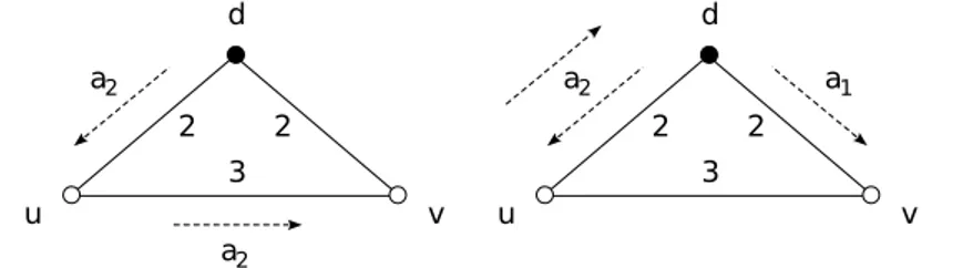
Consider the simple graph in Figure 3.1 with V = {d, u, v}.

Two agents a1 and a2 initially placed at the depot d have to perform two

d 2 3 u v 2 a₂ a2 d 2 3 u v 2 a₂ a₁

Figure 3.1: Instances of the problem in which the SUMDIST(·) objective (left) and the MAXTIME(·) objective (right) cannot be optimized simultaneously.

joint measurements defined by the set M = {(d, u), (d, v)}. By inspection, we can see that a solution S_D∗ minimizing the SUMDIST(·) objective is

SD∗ = [ha1 → d, a2 → ui, ha1→ d, a2→ vi],

with SUMDIST(S∗

D) = 7. Here, agent a1 remains fixed at d while a2 moves

to both u and v, eventually returning at d, with MAXTIME(S_D∗) = 7. Fo-cusing on the MAXTIME(·) objective, instead, we see (again by inspection) that an optimal solution S∗

T is

S_T∗ = [ha1 → d, a2 → ui, ha1→ v, a2→ di],

with MAXTIME(S_T∗) = 6 and SUMDIST(S∗_T) = 8. To optimize the latter objective, no agent remains fixed at the depot, at the expenses of an increase in the total traveled distance.

(30)

3.2 Complexity

NP-Hardness

The previous section defined the two optimization problems we are willing to solve. To prove that they are NP-hard, we use a reduction argument. Reducing problem A to another problem B means describing an algorithm to solve problem A under the assumption that an algorithm for problem B already exists. In order to show that our problem is hard, we need to describe an algorithm to solve a different problem, which we already know is hard, using it as a subroutine for our problem. The reduction implies that if problem A was easy, then problem B would be easy too. Equivalently, if problem B is hard, problem A must also be hard. Following this reasoning, if we demonstrate that the decision problems associated to our problems are NP-complete, we prove that the optimization version of our problems is NP-hard.

Suppose to have a solution S. The existence of two values D and T such that SUMDIST(S) ≤ D and MAXTIME(S) ≤ T can be verified in polyno-mial time by the algorithms2 _{(these two problems are named SUMDIST-D}

and MAXTIME-T from now on), therefore NP-membership is satisfied. In order to affirm that the two optimization problems related to the minimiza-tion of the SUMDIST(·) and the MAXTIME(·) objectives are NP-hard, we need to show that the SUMDIST-D and MAXTIME-T are NP-complete. This can be done by providing a reduction from the metric Traveling Sales-man Problem (TSP) which is known to be NP-complete [9].

B d B

v₁ v₂

G₁ G₂

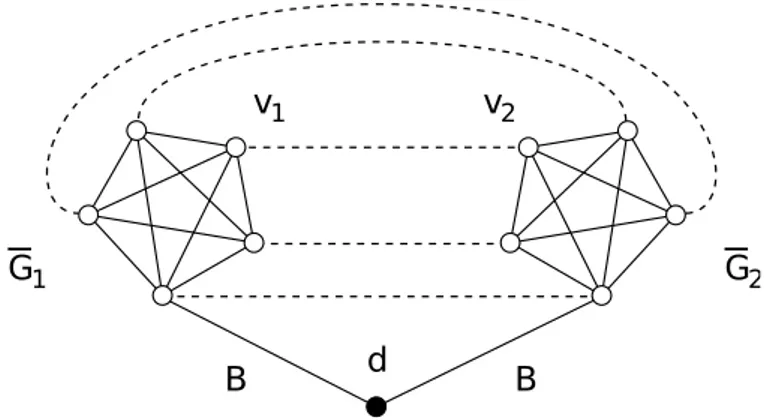
Figure 3.2: A reduction from a metric TSP instance with five vertices.

2

(31)

Let us consider first SUMDIST-D. From a generic instance of metric TSP, we construct a particular instance of SUMDIST-D with 2 robots and a graph G = (V, E) obtained as the metric closure of the graph shown in Figure 3.2. The metric closure of a weighted graph is a complete graph with the same vertices and in which edges are weighted by the shortest path distances be-tween corresponding vertices in the original graph.

In the figure, the original metric TSP graph is replicated twice in two subgraphs G1 and G2 which are connected to a depot d through the same

vertex copy with an edge with cost B. B is defined as the total distance of the Hamiltonian Cycle3 _{in G. We denote by v}

1, v2 the two vertices obtained

by replicating twice a generic vertex v ∈ V . The set of measurements is defined as M = {(v1, v2) ∀v ∈ V }, meaning that is composed by all the

pairs of vertices copies. Then we set D = 6B.

Consider a solution S of SUMDIST-D with SUMDIST(S) ≤ 6B in which two robots a1 and a2 starting from the depot d need to visit all the vertices

of a subgraph. The two robots initially reach G1 and G2, respectively

spend-ing B + B, then visit the vertices copies in the order defined by the metric TSP solution spending at most B + B, and finally travel back to the depot spending B + B. The total cost is not greater than 6B.

Consider now any solution S in which the measurement associated with the pair of vertices attached to the depot by means of the edge with cost B is not the first one performed. Since G (and hence G) is metric, S can always be turned into a solution in which such a measurement is the first one performed without increasing the total solution cost. Therefore, from such a solution, we can immediately derive the existence of a metric TSP solution with total distance at most B by examining the order in which the measurements are made.

The reasoning for the MAXTIME-T problem is the same, but we need to set the initial value of T to 3B. In this case we need to consider a solution S of MAXTIME-T with MAXTIME(S) ≤ 3B where two robots a1 and a2,

starting from d, firstly reach G1 and G2 spending B. Then they perform

time joint measurements visiting the vertices copies spending at most B, and return to the depot d spending B again. The total cost cannot exceed 3B.

Since we proved that the decision problems of SUMDIST-D and MAXTIME-T are NP-complete, their optimization version is NP-hard. Also, note that

3

A Hamiltonian Cycle is a closed loop in a graph that visits each vertex exactly once. 27

(32)

our proof shows that the problems remain NP-hard even on highly-restricted instances, namely, where m = 2 and each v ∈ V appears at most once in M .

Notation and Definitions

Table 3.1 summarizes the relevant terms and definitions presented. Some of them will be encountered in the following chapters.

M Set of the pairs of points in which a joint measurement is needed. It is given as input for the problem.

Configuration

Given a graph G = (V, E), a configuration is an assignment of m robots to m vertices on the graph.

Assignment

It is a tuple with: the robots that perform a measurement, the pair of points of the M set measured, and the cost of the measurement performed. E.g.: h(ai, aj); (vi, vj); c(·)i

ai, aj ∈ A, vi, vj ∈ M , c(·) according to the objective function we are

minimizing. Measurement Table

Table that stores the sequence of the assignment costs computed by the algorithms. See Section 4.2.

Move

Calculation of the search strategy of the algorithms that brings from a state to another. See Chapter 4.

(33)

Chapter 4

Algorithms

In order to tackle the problem introduced in the previous chapter, we im-plemented four algorithms which can be divided in two classes: graph ex-ploration algorithms, that we call K2 and K3, are those presented by [11], and informed search algorithms (Greedy and HBSS1_{) are instead two new}

algorithms devised for solving our problem.

The first section of this chapter presents the theoretical concepts be-hind the design of the informed search algorithms, the main contribution of this thesis to the field of study. The second section of the chapter aims at providing an exhaustive and precise explanation of the computations the algorithms perform.

4.1 Problem Framework

The computation of the most efficient tour can be related to a common process used in the field of Artificial Intelligence: state space search. The problem is modelled as finding the best sequence of states the problem can be in. Two states are connected if and only if an operation can be performed for shifting from the previous state into the one it is linked to. A state encodes the picture of the world (relevant to the problem) at a certain point along the progression of the plan, while the state space is the universe of all the possible states.

In a state only necessary information is encoded:

• Configuration of the team of robot: where each robot is located on the map.

1

This algorithm is based on the heuristic biased stochastic sampling technique intro-duced in Chapter 2.

(34)

• Measurement table: a table that stores for each robot the measure-ments performed up to that state. If we are minimizing time, it stores the time needed for each robot to reach the current configuration. If we are minimizing distance, it stores the sum of the distances each robot travelled from the beginning of the tour.

• Points to visit: the list of the pairs of points of the M set not yet visited.

The problem is formulated by specifying 5 elements:

• Initial state of the problem: in the initial configuration each robot is located at the depot, the measurement table is set to 0 for all robots, and the M set is complete. No measurement has been performed.

• Action(s): given the state s it returns the set of actions that are applicable in s. This means each possible joint measurement actuable from s, considering the pairs of points of M not yet visited.

• Result(s, a) = s′: is the function that returns the state reached per-forming action a in state s. The state s′ _{is a successor of s, action a}

belongs to Action(s). Hence, a successor state s′ is the state whose configuration is obtained by the application of action a to s.

• GoalT est(s): it is a Boolean function returning true if s is a goal state. A goal state corresponds to a state in which every pair of points of the M set has been visited.

• Cost(s, a): is the cost of performing action a in state s. Section 4.2 explains how costs are determined.

A solution to a search problem is a sequence of actions which brings from the initial state to one of the states that satisfy the goal test.

It is convenient to approach this search problem with a search tree. This allows us to understand and visualize better the problem. The search tree is a tree where the root corresponds to the initial state and the following pattern is repeated:

• Choose a state to expand.

• Apply the goal test to the chosen state.

(35)

Search Strategy

The definition of the search tree is not enough. Now we need to institute a procedure for the expansion of the states and search of the solution.

The first consideration to be made is that a complete expansion of the tree is not feasible, because it would lead to an expansion of useless states and, most importantly, taking into account the NP-hardness of the prob-lem2_{, would boost the computational complexity of the algorithm. Then,}

two other factors should be taken into account: completeness and optimal-ity. A strategy is complete if it is always able to find a solution (if a solution exists), and is optimal if it is guaranteed to find the minimum cost solution. The type of search strategy applied in the resolution of the problem could be linked to a typology of search strategy known in literature as uniform cost: the possible moves a state s can apply are sorted according to the cumulative costs up to s summed with the cost of the moves. The difference with the traditional strategy is that once a state is chosen, we expand it and consider the states that can be reached only from that state. In doing so, we do not keep track of the previously expanded state and so we cannot go back and see what the computation would have been if another action was chosen. This choice is justified by the complexity required by a complete expansion, which would require O(|M |!) steps.

Our search strategy is complete: we will always be able to find a solu-tion because we keep expanding states until each pair of points of the tour is visited.

Since after expanding a state we focus only on state space exploration deriving from that state, this search strategy can’t be optimal. To be cer-tain of the optimality of the solution, in fact, a complete search of the state space is needed: this approach though is not feasible in practice, as explained above.

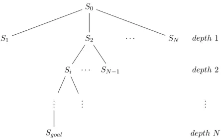
Figure 4.1 shows in practice the behaviour of the Search Strategy adopted.

2

See Chapter 3.

(36)

S0 S1 S2 Si .. . Sgoal .. . SN−1 SN depth 1 depth 2 .. . depth N · · · · · ·

Figure 4.1: Expansion of the search tree of the problem. Starting from the root S0,

the search strategy expands the state chosen until we reach a goal state. Notice that if |M | = N , we perform the action of expanding a state N times. Also, the states among which an expansion choice can be made depends on the depth level. Each expansion means that a pair of points of the tour has been visited, so the cardinality of the M set is reduced by 1 everytime a state is chosen. If the depth level is d (d ≥ 1) it means that we need to consider an expansion among N − (d − 1) states.

(37)

4.2 Algorithms

Input Data

Chapter 3 introduced the problem definition and formalization. Here, we recall the elements received as input by the algorithms.

G = (V, E) is a completely connected metric graph defined on n vertices. Each vertex v represents a location reachable by a robot. The team of m robotic agents A = ha1, a2, ..., ami can move between the vertices of G by

traveling along edges at uniform speed. The cost of each edge c : E → Z+

can represent either distances or traveling times between vertices. Since the graph is metric, the triangular inequality holds. The agents have to perform joint measurements on selected pairs of vertices M ⊆ E. With the term configuration we define an assignment of the m robots to m vertices on the graph. In the initial configuration each robot is assigned to the same starting position, the depot d.

Cost of Moves

Before the description of the algorithms, it is essential to accurately define how the cost of a move of the search strategy is calculated, since it is the basis for evaluating which joint measurement to perform next. A move is an action that brings from a state to another. The cost of a move represents the cost for shifting from a state to another and, therefore, from a configuration to another. In particular, the computation of the cost of a move for two robots ai and aj travelling from vertices vi, vj to vertices vk, vl depends on

the objective function we are considering.

• For MAXTIME(·) the cost of a move is computed as:

t = max{ti+ c(vi, vk), tj+ c(vj, vl)}3 (4.1)

• For SUMDIST(·) the cost of a move is computed as:

d = c(vi, vk) + c(vj, vl) (4.2)

In the MAXTIME(·) minimization the costs considered are the times needed to reach the vertices, while in the SUMDIST(·) minimization the costs are the distances between them. Equations 4.1 and 4.2 specify the notation introduced by Equation 3.1.

3

Recall that tiand tj are the costs of the time measurements performed by ai and aj

up to the state.

(38)

As stated in Section 4.1, evaluating moves means taking into account the smallest increase with respect to the objective functions. A practical exam-ple will clarify this reasoning.

Suppose to have four robots that after n steps have performed the fol-lowing measurements. Each value vi represents the cost incurred by robot

ai with respect to the objective function considered:

Obj. Function v1 v2 v3 v4

SUMDIST(·) 25 17 21 18

Obj. Function v1 v2 v3 v4

MAXTIME(·) 7 7 4 4

Suppose the moves that can be performed are the following (m1D and

m2Dfor the SUMDIST(·) objective function, m1T and m2T for the MAXTIME(·)):

Move Cost m1D 5 0 7 0 m2D 0 6 0 8 Move Cost m1T 3 0 2 0 m2T 0 0 1 5

The possible scenarios are:

• SUMDIST(·): m1D cost is 12, m2D cost is 14. Since the increase

brought by m1D in the objective function is lower, m1D is chosen. In

the SUMDIST(·) optimization evaluating moves is simple because the cost depends only on the sum of distances of the considered move.

• MAXTIME(·): m1T choice results in [10, 7, 10, 4]. m2T choice results

in [7, 7, 9, 9]. As outlined in Chapter 3, recall that in pairwise time-measurements a robot already occupying a vertex may be required to wait for a teammate to actually perform the measurement, which is the robot that induces the bottleneck time. That’s why in m1T robot

a3 timestamp is set to 10 and in m2T is set to 9.

Despite the bottleneck time of m2T (5) is higher than m1T (3), m2T is

chosen because it reflects a smaller increase in the objective function whose value is 9. With m1T its value would have been 10. As we can

see, the evaluation of a move in the case of MAXTIME(·) optimiza-tion is slightly more complex than SUMDIST(·) because we need to consider the history of the measurements performed by means of the measurement table.

4.2.1 Exploration Graph Algorithms: K2 and K3

After having defined the costs and the relative auxiliary data structures, we start with discussing two algorithms present in the literature [11]. We

(39)

call these algorithms K2 and K3 after the last name of one of the authors of [11]: Vijay Kumar. K2 stands for the 2-robot case, K3 for the 3-robot case, as we will see in this chapter. The core idea behind K2 and K3 is to compute the most efficient tour with the construction of an auxiliary data structure: the exploration graph.

Given a graph G = (V, E) and the M set, an exploration graph Gk =

(Vk, Ek) is created such that every vertex in v ∈ Vk denotes a k-robot

con-figuration on G that measures a subset of M . An edge eij_k ∈ Ek, exists

between two vertices vi k, v

j

k ∈ Vk, if the configuration associated to vki is

reachable from the configuration associated to vj_k. Being G a connected graph, k robots can always move from one configuration to another, making Gkcomplete. The cost assigned to every edge in Ekrepresents the minimum

cost for moving from one configuration to another.

We constructed an exploration graph only for the 2 and 3 robot cases (G2 and G3) because for an increasing number of robots it is an approach

poorly scalable and performing, since such a procedure would increase the complexity exponentially in the number of agents. The next sections will il-lustrate how the exploration graph is built and how it is used for computing a solution for the two scenarios.

K2 Algorithm

This algorithm can be used only if we have a team of 2 robots. In such case, K2 finds the optimal solution. The first step of the algorithm is to compute the vertex set V2 (Algorithm 1).

Algorithm 1 Vertex set V2 construction

input: environment graph G = (V, E), measurement set M output: a new set of vertices V2

V2= ∅

add v0

2 to V2 ⊲ v

0

2 denotes the vertex associated with d

foreach vertex vi in V do

foreach vertex vj in V do

if (vi, vj) ∈ M then

V2= V2∪ vx2 ⊲ vx2 denotes the vertex associated to vij

(40)

The main feature of constructing an exploration graph for the 2-robot case is that each vertex vi

2∈ V2 (v20 excluded) corresponds to one of the pair

of points of the M set where we want to perform a joint measurement. The weight of each edge eij2 ∈ E2 connecting two vertices v2i, v

j

2 ∈ V2 is obtained

by computing the minimum cost for moving from one vertex to another, which means the minimum cost for performing a measurement from one configuration to another.

Once the exploration graph is obtained, since each vertex vi

2 ∈ V2

cor-responds to a measurement that has to be carried out and since each edge eij₂ ∈ E2 represents the minimum cost that matches the cost of moving

two agents in the respective original problem, we can compute the solu-tion of a TSP4 _{on G}

2. The transformation outlined above is possible since

the presence of exactly two agents univocally identifies the optimal distance functions of the corresponding TSP.

In doing so, we reach an optimal solution for the 2-robot case of the problem.

K3 Algorithm

This algorithm can be used only if we have a team of 3 robots. [11] considered only non-weighted graphs. We extend the approach to cope with weighted graphs. The first step is the computation of the vertex set (Algorithm 2).

Algorithm 2 Vertex set V3 construction

input: environment graph G = (V, E), measurement set M output: a new set of vertices V3

V3= ∅

add v0

3 to V3 ⊲ v

0

3 denotes the vertex associated to d

foreach vertex vi in V do

foreach vertex vj in V do

foreach vertex vk in V do

if vi6= vj 6= vk then

if (vi, vj) or (vj, vk) or (vi, vk) ∈ M then

V3= V3∪ vx3 ⊲ v3xdenotes the vertex associated to vijk

4

(41)

The vertex set V3 represents all 3-robot configurations on the original

graph G = (V, E) that contain at least one pair of locations where a joint measurement needs to be performed. This means that a pair vi, vj ∈ M

might be associated with more than one vertex in V3 and a TSP cannot be

computed. The weight of each edge eij₃ ∈ E3 connecting two vertices v3i,

v₃j ∈ V3 is obtained by computing the minimum cost for moving from one

vertex to another, which means the minimum cost for performing a mea-surement from one configuration to another.

It’s important now to clarify a particular situation that might happen during the execution of K3. From the definition of the structure of the ex-ploration graph G3follows that in this algorithm robots can move singularly,

in pairs or even in triplets. In this way, a robot that moves from a vertex to another might not perform any measurement. Therefore, the measure-ment table needs to be updated carefully, especially for the MAXTIME(·) optimization:

• SUMDIST(·): the measurement table is updated only considering the distance costs resulting from the movement of the robots to their new positions.

• MAXTIME(·): the measurement table is first updated with the time costs resulting from the movement of the robots to their new position. Then it is updated considering the previous update and the bottleneck times of the robots performing the measurement.

The algorithm computation iterates over the following procedure: at each step the possible configurations reachable from the current one are calcu-lated and sorted. The sorting can be executed with respect to 3 different heuristics:

• Heuristic O: moves are sorted according to the cost. Ties are broken considering the minimum increase of the objective function.

• Heuristic C : moves are sorted according to how many measurements could be performed. Indeed, the definition of V3 suggests that moving

between two vertices vi 3 to v

j

3 implies that more than one measurement

might be completed. Ties are broken considering the Heuristic O.

• Heuristic H : moves are sorted according to the ratio between the cost and the number of measurements that would be performed. Ties are broken considering the minimum increase of the objective function.

(42)

Algorithm 3 K3 Algorithm

input: G = (V, E), initial configuration v0

3, heurisitic h, M set

compute G3= (V3, E3)

v3 = v 0 3

whileM is not empty do

V3list = vertices reachable from v3

sort V3list according to h and pick the first element v3best

delete from M the pairs of points included in v3best ⊲ *

v3= v3best

*: to make this instruction consistent, each heuristic considers only those moves that visit at least one element of the M set.

After sorting, the algorithm performs a greedy choice5 _{at each step until the}

M set is empty; the optimal plan for the 3-robot case results in a path over a subset of the vertices in V3. Preliminary experiments showed that if we

want to minimize MAXTIME(·) the best heuristic to use is H. Instead, if we want to minimize SUMDIST(·) the best heuristic is O.

4.2.2 Informed Search Algorithms: Greedy and HBSS The theory behind the developement of these two algorithms is outlined in Section 4.1: the search tree. When a state s is considered, starting from the initial state, three functions are sequentially executed:

1. EXPAND: computation of all the possible moves (and their costs) applicable from s.

2. CHOOSE : choice of the best move bm leading to the best assignment6_,

which is selected according to the algorithm considered.

3. GENERATE : creation of the state s′_{, generable from s after applying}

bm.

This procedure is repeated until every pair of points of the M set is visited. In each state it is encoded only necessary knowledge7 _{for the}

accomplish-ment of the operations described above.

5

A greedy choice is the selection of the element with the smallest incremental increase in the objective function according to the heuristic considered, with ties broken arbitrarily.

6

See Table 3.1.

7

(43)

These algorithms behave in the same way: in fact, Greedy is a special case of HBSS. The difference between them is the implementation of the CHOOSE function. The general algorithmic structure is described by Al-gorithm 4.

Algorithm 4 Informed search algorithms

input: G = (V, E), initial state S0, objective function obj, M set

ST AT ES = [S0]

S = S0

whileM is not empty do moves = EXPAND(S)

sort moves by minimum increase in obj chosen = CHOOSE (moves)

Snew= GENERATE (S, chosen)

add Snewto ST AT ES

delete from M the pair of points included in Snew

S = Snew

These algorithms can be run without restrictions on the number of robots composing the team. The next sections delineate a deeper explanation of the issues cited above.

Greedy Algorithm

In a greedy algorithm, the solution is progressively built from scratch. At each iteration, a new element is incorporated into the partial solution under construction, until a feasible solution is obtained and a goal is reached. The selection of the next element to be incorporated is determined by the eval-uation of all candidate elements according to a greedy evaleval-uation function. This greedy evaluation function represents the increment in the objective function after adding this new element into the partial solution. In a greedy setting, we select the element with the smallest incremental increase (re-member that objective functions are costs, in our application), with ties broken arbitrarily. Costs are evaluated as outlined in Section 4.2.

These properties are embodied within the Greedy Algorithm which it-eratively expands a state (EXPAND) and, after sorting the moves by the minimum increase in the objective function considered, chooses the first element which corresponds to the best one according to the greediness cri-terion (CHOOSE ) and generates the corresponding state (GENERATE ).

(44)

The Greedy Algorithm is guaranteed to find a feasible solution, since, for this problem, a greedy approach can easily be shown to be complete. However, solutions obtained by greedy algorithms are not necessarily opti-mal but their performance can boost if we allow the algorithm to explore states in addition to those suggested by the greedy choice. This is the con-cept behind the implementation of the next algorithm.

HBSS Algorithm

The HBSS Algorithm idea is designed around the sampling methodology described in [6]. As mentioned before, a greedy choice throughout the ex-pansions of states is highly probable that does not lead to optimal solutions. A different exploration of the space state, instead, might tend to the discov-ery of a better solution and, theoretically, even to the optimal one.

We can explore the state space in a more significant way with respect to the greedy choice thanks to randomization. Randomization plays an impor-tant role in algorithm design, especially when sampling the state space.

Greedy randomized algorithms are based on the same principle guiding pure greedy algorithms but they make use of randomization to build dif-ferent solutions at difdif-ferent runs. At each iteration, the set of candidate elements is formed by all elements that can be incorporated into the partial solution under construction without violating feasibility. The selection of the next element is determined by the evaluation of all candidate elements according to a greedy evaluation function.

The evaluation function applied in the HBSS Algorithm derives from a technique called heuristic biased stochastic sampling8_{. This methodology}

doesn’t sample the state space randomly but it focuses its exploration using a given heuristic, which in our case is the greedy one. The adherence to the heuristic depends on another component, the bias function. The bias function selection has consequences on the state space exploration depend-ing on the confidence placed in the heuristic: the higher the confidence, the stronger the bias, therefore fewer solutions different from the greedy one are produced. On the other hand, a weaker bias implies a greater degree of exploration since we are not attached to the heuristic; this leads to a higher variety of solutions.

A complete solution is generated starting from the root node and se-lecting at each step the node sampled by the HBSS state space exploration procedure, until all pairs of points in the M set are visited, meaning that

8

(45)

a goal node is reached. In order to select a node, the candidate elements are sorted according to the heuristic (e.g., greedy) and a rank is assigned to each candidate, based on the ordering - top rank is 1. The bias function is used to assign a non-negative weight to each candidate based on its rank. After normalization, the normalized weight represents the probability of the candidate of being selected. Notice that each candidate has a non-zero prob-ability of being chosen at each step.

Algorithm 5 shows the pseudocode relative to how the CHOOSE func-tion changes with respect to the Greedy Algorithm. The general structure regarding EXPAND and GENERATE functions still holds.

Algorithm 5 CHOOSE Function - HBSS Search

input: G = (V, E), heuristic function h, bias function b, state s, M set9

children = sorting based on h of moves totalW eight = 0

foreach child in children do

rank[child] = position in children ⊲ top rank is 1 weight[child] = b(rank[child])

totalW eight = totalW eight + weight[child] end for

foreach child in children do

probability[child] = weight[child]/totalW eight end for

index = weighted random selection based on probability chosen = children[index]

The HBSS Search algorithm will find a feasible solution sampling the state space with the operations depicted above. Notice that the difference with the Greedy Algorithm lies in the choice of the move to apply, which might not be the first one in the sorted list (children). The given result might be better or worse than the solution found by the greedy one, depending on how we choose the bias function and also by how many outcomes are calculated. In fact, another strength of the heuristic biased stochastic sam-pling technique is that we can iterate over the number of times we compute a solution through HBSS Search.

9

Even if in this pseudocode some input data are not used, this list is consistent with the function call actually made by the HBBS Algorithm - see Algorithm 6.

(46)

HBSS Search runs until a feasible and complete solution is determined. If this process is repeated N times we would obtain a wider exploration of the state space because at each iteration, a complete HBSS Search pro-cedure is carried out. With a proper tuning of the bias function, a wide collection of different solutions is likely obtainable and, with an extended range of solutions to consider we have higher probabilities to reach optimal-ity (Algorithm 6).

Algorithm 6 HBSS Algorithm

input: G = (V, E), heuristic function h, bias function b, initial state S0, M set,

number of restarts N : RESU LT S = [ ] HBSS(N, S0, h, b):

fori in range (0, N ) do

res = HBSS-Search(S0, h, b)

add res to RESU LT S end for

In RESULTS is stored each of the N computations of a complete run of the HBSS Search procedure. The minimum value over the instances of the list is the best result calculated.

The iterative sampling performed by the HBSS approach depends on the definition of the bias function, that might encompass greedy search and completely random search as extreme members. The bias functions (r is the rank) considered in this work are:

• logarithmic: bias(r) = log−1(r + 1) • polynomial(τ ): bias(r) = r−τ • exponential : bias(r) = e−r

From preliminary experiments the best bias function typology is the poly-nomial. Chapter 7 will focus on the analysis of the tuning of a proper polynomial degree and of its performance.

(47)

Computational Complexity

From the results of Chapter 3 it is clear that, unless P=NP, the existence of polynomial-time optimal algorithms for any of the two objectives is improb-able. However, for the special case of a team of two robots, there exist two simple polynomial-time transformations from our optimization problems to particular TSP instances, for which advanced solvers exist [1].

For what concerns the HBSS Algorithm, if we assume that an assign-ment of the team of robots to a configuration can be evaluated in a constant number of steps, each solution can be found in O(m2_{|M |}2_{log m|M |) steps,}

implying that, if the number of runs is polynomial in the input size, the whole algorithm has a polynomial running time. This complexity derives from the fact that for each step in the evaluation of the assignments (the total number of steps before algorithm completion is |M |), the cost of each move is computed in O(m2_{|M |) and then sorted in O(log m|M |). Repeating}

this process |M | times we obtain O(m2_{|M |}2_{log m|M |).}

Approximation Factor

We now provide a result that could be useful in the study of an approxima-tion factor for the Greedy Algorithm.

Let Algorithm 1D be the Greedy Algorithm in charge of SUMDIST(·)

optimization. We put in relation the maximum cost of a greedy assignment and the cost of an optimal solution.

Let SDbe a solution found by Algorithm 1Dwith M = E, and let OPTD

be the cost of an optimal solution minimizing the SUMDIST(·) objective function. Then,

max

sk∈SD

c(sk) ≤ 2 OPTD.

Proof. Consider a single depot multiple traveling salesmen problem (m-TSP) on G, with m salesmen and a depot d. In this problem, the goal is to find a set of m tours, each starting from d and visiting at least once every vertex in G, such that the sum of the tour costs is minimized. Let Cmtsp be the cost

of the m-TSP optimal solution. Since in our problem each vertex must be visited at least once, it follows that Cmtsp ≤ OPTD. Then, let Cmst be the

cost of a minimum spanning tree10 _{on G. We have C}

mst ≤ Cmtsp, because

from any m-TSP solution a spanning tree can be obtained by removing the last tour edges (the ones returning to the depot). Finally, the cost between

10

A minimum spanning tree is a least cost tree covering all the vertices in a graph. 43

(48)

any pair of vertices in G cannot be greater than Cmst, because of the triangle

inequality. Reconstructing the chain of inequalities we have that the sum of the costs of the greedy assignment can never exceed twice OPTD.

(49)

Chapter 5

System Architecture

5.1 Systems Involved

Computing efficiently multirobot paths for performing joint measurements can be employed in several applications, as already discussed in Chapter 2. In this chapter we describe the system architecture developed for such computation.

We start from a known environment, therefore a physical map is needed. The pairs of points where we would like to perform joint measurements are then chosen on that map and the algorithm, after receiving this information, can start computing the most efficient tour providing the best solution ac-cording to the selected objective. This is how the workflow is formed from an abstract point of view; technically the process is more complex and the final output of the algorithms (an m-robots tour) is obtained by the combination of three systems:

• System 1: data acquisition.

• System 2: data processing and solution computation.

• System 3: analysis of the results and experiments on performance of the algorithms.

Figure 5.1 depicts the workflow in which the three systems are involved. The next sections will give a deep explanation of each system’s tasks.

(50)

Figure 5.1: Systems interactions.

5.1.1 System 1: Acquiring Data

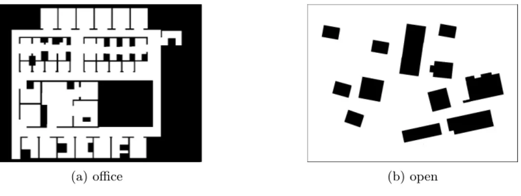
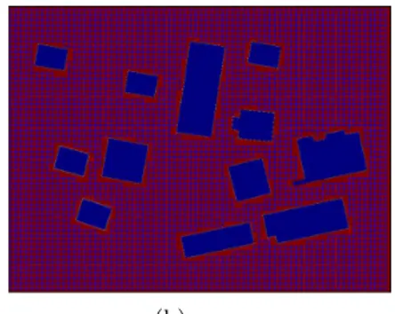
In this system there are three main entities: environments, graph scripts, and data. It all starts with a physical map of the environment which is encoded as a 800x600 .png file. In this work the environments1 _{used were}

two; from now on they will be referred to as office and open. These are also the environments which will be used in the experiments of Chapter 6. In the map representations shown in Figure 5.2, robots can move on the white pixels, while black pixels represents obstacles or unacessible points.

(a) office (b) open

Figure 5.2: Environments - png files.

1

The environment maps were downloaded from Radish, a robotics data set repository. (radish.sourceforge.net)