An algorithm for the generation of all possible combinatorial multivector fields on cubical complexes

(1)

SCUOLA DI SCIENZE

Corso di Laurea Magistrale in Informatica

An algorithm for the generation of all

possible combinatorial multivector

fields on cubical complexes

Relatore:

Chiar.mo Prof.

Massimo Ferri

Presentata da:

Stefano Pisciella

Correlatore:

Dott.

Mateusz Juda

Correlatore:

Chiar.mo Prof.

Giulio Casciola

Sessione II

Anno Accademico 2016/2017

(2)

(3)

(4)

Introduzione

La topologia computazionale `e un campo di studio emergente che si po-siziona nell’intersezione tra la matematica, in particolare la topologia, e l’informatica. Lo scopo primario `e quello di sviluppare algoritmi che uti-lizzino strutture dati topologiche al fine di risolvere in maniera efficiente problemi riconducibili alla topologia.

I ricercatori della facoltà di Matematica ed Informatica dell’Università Jag-ellonica di Cracovia hanno recentemente sviluppato una struttura dati [1], chiamata combinatorial multivector field, dimostrandone importanti carat-teristiche topologiche. Data la recente introduzione, non vi sono presenti lavori ufficiali che utilizzano questa nuova struttura. Nonostante questo i ricercatori di Cracovia stanno lavorando su diversi progetti al fine di mostrare le interessanti proprietà per quanto riguarda, soprattutto, lo studio di sistemi dinamici.

Il seguente lavoro di tesi si inserisce in uno di questi progetti, che si propone di fornire un metodo per studiare in maniera efficiente il comportamento dinam-ico di geni e proteine, attraverso l’associazione dei gene regulatory networks con la struttura topologica da loro sviluppata.

Lo scopo di questo lavoro `e quello di definire, insieme ad una formale vali-dazione matematica, un algoritmo per la generazione di tutti i combinatorial multivector fields su una particolare struttura topologica chiamata cubical complex.

Nella prima parte si vedranno concetti matematici necessari per capire il resto della tesi. Seguir`a la definizione formale dell’algoritmo fulcro della

(5)

tesi. Si analizzeranno poi due implementazioni realizzate da noi per il test e l’esecuzione finale. Infine verranno analizzati i risultati dei test e i dati finali che verranno utilizzati per il successivo sviluppo del progetto.

(6)

Introduction

Computational topology is an emerging field of study which could be con-sidered a subfield of topology and some areas of computer science. The main goal is to develop efficient algorithms, which use topological structures, in order to solve problems that can be associated to topology.

The researchers of the Faculty of Mathematics and Computer Science at the Jagiellonian University of Krakow have recently developed a new data struc-ture, called combinatorial multivector fields, proving some important topo-logical features of it. Due to the recent development, there are still not any official works using that structure. Nevertheless, the researchers are working on several projects in order to show the interesting properties, mostly related to the study of dynamic systems.

This work is part of one of those projects, which aims to provide an efficient and interactive way to study the dynamic behaviour of genes and proteins using a link between gene regulatory networks and the data structure they defined.

The goal of this dissertation is to define, together with a formal mathematical validation, an algorithm for the generation of all possible combinatorial mul-tivector fields on a particular topological structure called cubical complex. In the first part of the work we will give some preliminary concepts to better understand the rest of the work. We proceed, then, giving a formal definition of our algorithm followed by the analysis of two different implementations we developed. Finally we will give some interesting information about our tests and the final data we produced.

(7)

(8)

List of Figures

1.1 Example of elementary cubes . . . 3

1.2 Example of a cubical complex . . . 5

1.3 Example of a labelled cubical complex . . . 6

1.4 A cubical complex represented by its Hasse diagram . . . 7

1.5 Example of proper and improper sets . . . 8

1.6 Example of proper and improper sets using the Hasse diagram representation . . . 8

1.7 Example of a combinatorial multivector field together with an improper partion . . . 10

2.1 A graphic representation of a CTree . . . 13

2.2 Transition between combinatorial multivector fields and rela-tive configurations . . . 17

2.3 A graphic representation of a PCTree . . . 20

3.1 Example of a Thomas network . . . 26

3.2 Data structure used to represent proper configurations . . . . 28

3.3 Graphical explaination of a proper check algorithm property . 32 3.4 Results of the tests about time performance . . . 37

3.5 Results of the tests about disk occupation . . . 38

(11)

(12)

List of Tables

3.1 Parameters used for testing purpose . . . 36

(13)

(14)

Chapter 1 Preliminaries

In this chapter we introduce notations and definitions used in the sequel, mostly taken from [1, 2, 3].

1.1 Lefschetz Complex

The definition given below represents an abstract topological structure. In this work we are interested in a particular structure which suits that defini-tion. Therefore, in the next section, we are going to introduce that structure, showing concrete example to better understand the notions introduced in this section. The following definition is the same used in [1] and given in [3]. Definition 1.1.1. Let R be a fixed ring with unity, (X, k) is a Lefschetz complex if X = (Xq)q∈Z+ is a finite set with gradation, k : X × X → R is

a map such that k(x, y) 6= 0 implies x ∈ Xq, y ∈ Xq−1 and for any x, z ∈ X

we have

X

y∈X

k(x, y)k(y, z) = 0

The elements of X are called cells and k(x, y) is the incidence coefficient of x, y.

Given x, y ∈ X, y is a facet of x, and write y ≺k x, if k(x, y) 6= 0. The

(15)

relation ≺k extends uniquely to a minimal partial order denoted by ≤k and

the associated strict order by <k. y is a face of x if y ≤k x.

1.2 Cubical Complexes

The following definitions are given in [4, 5].

Definition 1.2.1. An elementary interval is a closed interval I ⊂ R of the form

I = [l, l + 1] or I = [l, l]

Definition 1.2.2. An elementary cube Q is a finite product of elementary intervals

Q = I1× I2× · · · × Id ⊂ Rd

Examples of elementary cubes are shown in Fig.1.1.

The dimension of an elementary cube Q is given by the number of non degenerate intervals, which are those intervals in the form [l, l + 1], in the product decomposition.

The j th nondegeneracy number of Q is defined by v(Q, j) :=

  

card{i < j | dim Ii = 1} if dim Ij = 1,

0 otherwise.

Definition 1.2.3. A cubical complex C in Rdis a finite collection of elemen-tary cubes in Rd

As example of a possible incidence coefficient k on a cubical complex C we have

(16)

1.2 Cubical Complexes 3

Figure 1.1: Elementary cubes in R2_{. The cube A = [2, 2] × [3, 3]. The cube}

B = [1, 2] × [1, 1]. The cube C = [3, 4] × [1, 2]. k(Q, P ) :=                        (−1)v(Q,j) if Q = I1× · · · × Ij × · · · Id and P = I1× · · · × Ij−× · · · × Id, (−1)1+v(Q,j) _{if Q = I} 1× · · · × Ij × · · · Id and P = I1× · · · × Ij+× · · · × Id, 0 otherwise. with Q, P ∈ C.

The definition of cubical complex, along with a function which indicates the incidence coefficient between two elements of the complex, is compatible with the one of Lefschetz complex. The proof of that, which does not concern this work, can be found in [4, 5].

(17)

For the purpose of this work, we need to analyse only specific cubical com-plexes in R2, thus every cubical complex used in the rest of the work is implicitly in R2.

Let C be a cubical complex.

We can identify three kinds of possible elements, also called cells, in C: • vertices, 0-dimensional elementary cubes or 0-cells.

• edges, 1-dimensional elementary cubes or 1-cells. • squares, 2-dimensional elementary cubes or 2-cells.

The cubical complexes we are analysing are those composed by adjacent squares along with the edges and the vertices that compose them. Graphi-cally speaking, they should be represented by a grid. Namely, the smallest one is a grid 1 × 1 with a square, 4 edges and 4 vertices. An example is shown in Fig.1.2.

To make it more readable and easier to explain we change the notation used so far for the cubical complex.

First of all, we use a grid notation for specifying the size of a cubical complex. Namely if we are working with a 1 × 2 cubical complex C, it means C is composed by two squares, seven edges and six vertices. Graphically speaking, C could be represented as two squares in a row.

We use the notation length of a n × m cubical complex C to indicate the number of cells belonging to C. Which is

length(C) = (2n + 1) · (2m + 1)

We will no longer use the notation of elementary cubes to address the ele-ments. Instead we are going to use an incremental index, which goes from the left to the right, from the top to the bottom. The indexes of the cells belonging to C are in [ 0 , . . . , length(C) − 1]. Note that, in that way we can avoid using the Cartesian plane to graphically represent a cubical complex. An example is shown in Fig.1.3.

(18)

Figure 1.2: A cubical complex C in R2_{. The vertices are marked by a green}

dot. The edges are marked by a blue line. The squares are marked by a grey square. C is composed by 4 squares, 12 edges and 9 vertices.

Given A ⊆ C, the closure of A, we write closure(A), is a set containing A, the facets of cells in A, the facets of the facets of cells in A and so on. In this context, it is easy to recognize the facets of a cell c ∈ C

• If c is a square then the facets of c are the four edges at the borders of c.

• If c is an edge then the facets of c are the two vertices at the extremities of c.

• If c is a vertex then it has no facet.

(19)

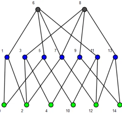
represen-Figure 1.3: A 1 × 2 cubical complex C of length 15. Every cell is marked with a circle in its centre of mass and with its index. The green dots indicate the vertices, the blue dots indicate the edges and the grey dots indicate the squares.

tation of a cubical complex, as it is a poset1_{, as shown in Fig.1.4. In that}

view both closure and facets are easy to be observed. In fact, the facets of a cell are the cells you can reach from the cell by going down one level. The closure of a cell is the set composed by the cell itself and all the cells you can reach going down trough the diagram.

A is closed if closure(A) = A. A is proper if closure(A)\A is closed.

An example is given in Fig.1.5. In our setting, proper sets correspond to convex sets in the language of the associated partial order, induced by k. That is why, even in this case, it is probably easier to show that property with the Hasse diagram shown in Fig. 1.6. Namely a set is proper if there does not exist a path, which goes only from the bottom to the top, that joins any two elements of the set passing through an element which is not in the

1_{A poset consists of a set together with a binary relation indicating that, for certain} pairs of elements in the set, one of the elements precedes the other in the ordering. Here the binary relation is the incidence coefficient function.

(20)

Figure 1.4: The Hasse diagram of a 1 × 2 cubical complex C.

(21)

Figure 1.5: A 1 × 2 cubical complex C. Two subsets of C are indicated by a black ellipse, A = {0, 1} and B = {4, 8}. The closure of A {0, 1, 2} is surrounded by a red dotted ellipse. The closure of B {2, 3, 4, 7, 8, 9, 12, 13, 14} is surrounded by an orange dotted ellipse. A is a proper set, while B is not.

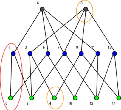
Figure 1.6: The Hasse diagram of a 1 × 2 cubical complex C. The same two subsets of the Fig.1.5 are indicated on the graph. The set B = {4, 8} is improper because there are path which joins the elements passing out of the set e.g. the path 4 - 9 - 8, the cell 9 /∈ B.

(22)

1.3 Combinatorial multivector fields 9

1.3 Combinatorial multivector fields

The following definitions are given in [1]. Let (X, k) be a fixed Lefschetz complex.

Definition 1.3.1. A combinatorial multivector is a proper subset V ⊆ X admitting a unique maximal element with respect to the partial order ≤k.

We call this element the dominant cell of V and denote it V∗.

Specifically, given a cubical complex C, a combinatorial multivector, or briefly multivector, V is a proper subset of C which can contain a unique maximal element. In other words:

• If the maximal element of V is a 2-cell then if V contains other cells, those could be just edges and/or vertices.

• If the maximal element of V is a 1-cell then if V contains other cells, those could be just vertices.

• If the maximal element of V is a 0-cell then V does not contain any other cell.

Note that the maximal element is defined considering the partial order rela-tion, that means, among other things, a multivector can contain just adjacent cells.

It is easy to see that for every multivector V

closure(V ) = closure(V∗).

Definition 1.3.2. A combinatorial multivector field on X is a partition V of X into multivectors.

In our context, a combinatorial multivector field is a partition of C into multivectors. That is a set of proper subsets of C each one admitting a unique maximal element.

(23)

Figure 1.7: On the left a partition of a cubical complex 1 × 2 which is not a combinatorial multivector field. In fact, the subset {11, 12, 13} is proper but has two maximal elements while the subset {3, 4, 8} is not proper, they are both not multivectors.

On the right a combinatorial multivector field as a partition of the same cubical complex.

(24)

Chapter 2 Combinatorial multivector field

generation algorithm

The current chapter is the main part of the work, here we present, and validate, our algorithm which generates all the possible combinatorial multi-vector fields on a cubical complex.

2.1 Configuration

Definition 2.1.1. Given a cubical complex C, we define a partial configura-tion on C as an oriented graph G = (V, E) such that:

1. V = C.

2. For each e = (i, j) ∈ E we have: (a) i ∈ closure(j).

(b) @(i, k) ∈ E such that k ∈ V and k 6= j. (c) @(j, k) ∈ E such that k ∈ V and k 6= j.

The three conditions grant that every edge goes from a cell c to the cell itself or to another cell with higher dimension (condition 2.a), that every cell has at maximum one outbound edge (condition 2.b) and that if a cell has an

(25)

inbound edge it can be connected just to itself (condition 2.c).

The length of a partial configuration, denoted by length, is the number of nodes with an outbound edge.

We indicate with PCC the set of all the partial configuration on a cubical

complex C.

If P C = (V, E) ∈ PCC and length(P C) = |V | then P C is a configuration,

namely a partial configuration is a configuration if it has an outbound edge for every vertex.

Definition 2.1.2. Given a cubical complex C and a partial configuration P C = (V, E) ∈ PCC with length(P C) < |V | we define a function

move(i,j)(P C) = P C0

such that P C0 = (V, E0_{) ∈ PC}C and E0 = E ∪ {(i, j)}, (i, j) /∈ E.

Note that every partial configuration P C, which is not a configuration, has at least |V | − length(P C) possible moves.

We now want to generate all configurations on a n × m cubical complex C. To do so, we build a tree CTC = (PCC, E), following these steps:

1. The root of the tree represents the empty partial configuration i.e. a partial configuration with length 0.

2. For each node PC at level1 _{l ∈ [1, . . . , length(C)] we generate as many}

children as the possible different moves in the form of move(l−1,j)(P C),

with j ∈ [1, . . . , length(C)]. We call CTC the CT reee of C.

Note that depending on the order in which the moves are analysed we can create different trees. As far as this work is concerned, we can consider those trees to be equivalent.

1_{The level of a node is 1+ the number of edges within the path from the root to the} node.

(26)

2.1 Configuration 13 In Fig.2.1 we show a CTree of a small cubical complex; it is rather hard to show the complete Ctree of a 1 × 1 cubical complex.

Algorithm 1 shows a simple way to build the above-mentioned tree in a depth-first like approach.

Figure 2.1: A Ctree of a cubical complex C, subset of a 1 × 1 cubical com-plex, composed by the labelled cells i.e. {0,1,2,3}. The labels of the nodes represent the cell currently analysed. The labels of the edges represent the cell to which the analysed element is going to connect.

(27)

Algorithm 1 Visit of the CTree function GenerateCTree(n, m)

CubicalComplex ← A n × m cubical complex

P C ← A partial configuration on CubicalComplex without any edges VisitCTree(0, P C)

end function

function GenerateSubCTree(Cell, P C)

neighbours ← {c | ∃P C0such that P C0 ← move(Cell,c)(P C)}

for each neighbour in neighbours do P C0 ← move(Cell,neighbour)(P C)

if Cell is not the last cell then

GenerateSubCTree(Cell + 1, P C0) end if

end for end function

Let C be a cubical complex and CTC a CTree of C.

Proposition 2.1.1. Every node of CTC represents a different partial

config-uration.

Proof. By construction of the CTree, we already know that every node of CTC is a partial configuration. That is because we move from a node to the

next one using the function move.

Taking any two different nodes P C, P C0 to show that they represent two different partial configurations, we have to analyse the following cases:

• P C and P C0 _{are at level l and l}0_{, respectively, with l 6= l}0_{. Let’s say}

l > l0. In that situation, we can be sure that P C contains at least one edge that P C0 does not have. For instance, the edge that connects the cell l − 2 with some other possible cell. If l0 > l we can apply the same reasoning. Therefore P C 6= P C0.

(28)

2.1 Configuration 15 are obtained choosing two different moves from the partial configuration represented by their father.

On the other hand if they have two different fathers, we can go through their ancestors until we find a common one. At that point we can apply the same reasoning of the common father situation.

Proposition 2.1.2. The leaves of CTC represent all and only the possible

configurations on C.

Proof. We have to highlight that the leaves are at level p + 1 where p = length(C). Therefore all the partial configurations represented by the leaves contain an edge for every cell ∈ {0, ..., p − 1}, that is they have an edge for each cell ∈ C. In other words, every leaf is a configuration.

It remains to prove that there does not exist a configuration which is not represented by a leaf.

Let c be a configuration which is not in the leaves, therefore c has at least one edge different from every leaf of the tree. We can order the edges in c by their source node:

{(0, u0), (1, u1), . . . , (i − 1, ui−1), (i, ui), . . . , (p − 1, up−1)}

Let (i, ui) be the edge that does not belong to any leaf. We can easily follow

the path indicated by the first i edges in the tree, from the root of CTC to the

node at level i end point of the edge (i − 1, ui−1). At that point, by definition

of CTree, we are going to generate a node for every possible different moves of the type move(i,j) for every suitable j. Therefore if c is a configuration, ui

is suitable accordingly c is not a configuration.

As we are able to generate all possible configurations on a cubical complex, we now want to create a mapping between a combinatorial multivector field and a configuration.

(29)

multivector field. To do that, given a CMF CV on a cubical complex C, we build a graph G = (C, E) such that:

1. For each cell c ∈ C we add the edge (c, [c]∗_CV) in G, where [c]∗_CV indicates the dominant cell of the multivector which c belongs to.

The vertices of G are the cells of the cubical complex C, which is the condi-tion 1 of the definicondi-tion 2.1.1.

Moreover every edge of G goes from a cell c to the dominant of the multi-vector to which c belongs. That means every edge goes from c to c itself or an higher dimensional cell, which is the condition 2.a of the definition 2.1.1. As the dominant is unique, there exists just one outbound edge for each cell which is the condition 2.b of the definition 2.1.1.

If a vertex c of G has an inbound connection, it means c is the dominant of its multivector. Therefore it can have just an outbound connection to itself, which is the condition 2.c of the definition 2.1.1.

G respects the definition 2.1.1 in particular, as length(G) = length(C), G is a configuration. We call G the relative configuration of CV .

Theorem 2.1.1. Given a cubical complex C, let CTC be the CTree of C.

If CV is a CMF on C then there exist one and only one leaf of CTC which

represents the relative configuration of CV .

Proof. The proof is obvious because of the properties we have showed so far. In fact we know that it is always possible to create a configuration from a CMF, furthermore we have already proved that the leaves of a CTree represent all and only the possible configurations.

2.2 Proper configuration

Although we are now able to generate all the possible CMF on a cubical complex, there still exists a challenging problem. Namely computing all the configurations on a cubical complex, even of small size, could require lot of

(30)

2.2 Proper configuration 17 resources. We will show some evidence in the next chapter.

We have previously seen that every combinatorial multivector field could be translated in a configuration, but the opposite is not true as showed in Fig.2.2. The problem here is that configurations, as they are defined, allow improper set.

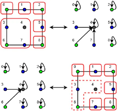
Figure 2.2: On the top, a transition from a combinatorial multivector field {{0}, {1}, {2}, {3, 4, 6, 7}, {5}, {8}} to its relative configuration. On the bot-tom a configuration is shown, which cannot be translated in a combinatorial multivector field, the multivector indicated by the dotted quadrilateral is not proper. Both examples are based on a cubical complex 1 × 1.

Definition 2.2.1. Given a cubical complex C, we define a proper partial configuration as a partial configuration P P C with the following constraint:

• Let UP P C be the underlying undirected graph of P P C. For each component M V = (V, E) of UP P C, V represents a proper set on C.

(31)

n

In the same way, a proper partial configuration is a proper configuration if it has an outbound edge for every vertex.

We indicate with PPCC the set of all proper partial configurations on a

cubical complex C. Obviously PPCC ⊂ PCC.

With relative CMF of a proper configuration P P C on a cubical complex C we indicate a combinatorial multivector field M V on C such that:

• Let UP P C be the underlying undirected graph of P P C. The set of nodes of every component of UP P C represent a multivector in M V It is easy to see that every combinatorial multivector field has its relative proper configuration and that every proper configuration has its relative CMF. It is a one-to-one relation.

Definition 2.2.2. Given a cubical complex C, P P C = (V, E) ∈ PPCC with

length(P P C) < |V | we define a function

pmove(i,j)(P P C) = P P C0

such that P P C0 = (V, E0_{) ∈ PPC}C and E0 = E ∪ {(i, j)} with (i, j) /∈ E.

As we have previously done with the configurations, we now want to generate all proper configurations on a n × m cubical complex C. To do so, we build a tree P CTC = (PPCC, E), following these steps:

1. The root of the tree represents the empty partial configuration, the same root of CTC.

2. We create a list cells of the cell of C ordered by their dimension, i.e. first of all squares followed by edges and vertices.

3. For each node PPC at level l ∈ {1, . . . , length(C)} we generate as many children as the possible pmoves in the form of pmove(cells[l−1],j)(P C).

(32)

2.2 Proper configuration 19 Note that the elements of the list cells in the tree construction are addressed by index starting from 0 to length(C) − 1.

We call P CTC the P CT ree of C. As the CT ree, depending on the order in

which the moves are analysed, we can create different trees. But still, we can consider those trees equivalent.

In algorithm 2 is shown a simple way to build the PCTree in a depth-first like approach.

Algorithm 2 Visit of the PCTree function generatePCTree(n, m)

CubicalComplex ← A n × m cubical complex

P P C ← A partial configuration on CubicalComplex without any edges cells ← A list of C’s cells ordered by their dimension

VisitPCTree(0, P P C, cells) end function

function GenerateSubPCTree(index, P P C, cells)

neighbours ← {c | ∃P P C0_{such that P P C}0 _←

pmove(cells[index],c)(P P C)}

for each neighbour in neighbours do P P C0 ← pmove(cells[index],neighbour)(P P C)

if cells[index] is not the last cells’ element then GenerateSubPCTree(index + 1, P P C0, cells) end if

end for end function

The main idea here is the order of the list of cells. In fact, as we will show later, that order will allow us to cut some branches of the tree because of the proper property.

Let C be a n × m cubical complex and P CTC a PCTree of C.

Proposition 2.2.1. Every node of P CTC represents a different proper

(33)

Proof. That property is inherited from the CTree. In fact the PCTree is a CTree in which we cut some branches, because of the proper property, and we move to the next levels with the pmove functions. Therefore it’s obvious that every node represents a different proper partial configuration.

In Fig.2.3 we show a PCTree of the same cubical complex used in Fig.2.1. Note that, following the path from the root to the leaves without considering the cuts, the leaves of the tree are the same of the CTree in 2.1, regardless of their order.

Figure 2.3: A PCtree of a cubical complex C, subset of a 1 × 1 cubical complex, composed by the labelled cells i.e. {0,1,2,3}. The labels of the nodes represent the cell currently analysed. The labels of the edges represent the cell to which the analysed element is going to connect. The cross indicates that that branch is cut because of an improper state, which is reached adding the edge (0, 3) to the proper partial configuration represented by the path from the root the the leaf father of the branch cut.

Proposition 2.2.2. The leaves of P CTC represent all and only the possible

(34)

2.2 Proper configuration 21 Proof. The fact that ever leaf of P CTC is a proper configuration is obvious,

it comes directly from the same proof for the CTree.

Suppose P P C be a proper configuration which does not belong to the leaves of P CTC. In other words, the branch where P C belonged was cut because

of an improper state. Ordering the edges in P P C by the dimension of their source cell we have:

{(i1, i1), . . . , (in, in), (j1, x1), . . . , (jm, xm), (k1, y1), . . . , (kp, yp)}

where i indicates the squares cells, which are always connected to themselves, j indicates the edges and k indicates the vertices.

It is easy to see that a set composed only by a square or by a square and edges is always proper. Therefore an improper state is reached adding one of the last p connections.

Let (kq, yq), with q < p, be that connection, P C a partial configuration

composed by the first n + m + q edges of P P C and V the component of the underlying undirected graph of P C, which represents an improper state. Accordingly, by the definition of closure, we know that ∃j∈C such that:

∃k, i∈V k ∈ closure(j), j ∈ closure(i), j /∈ V

where j is, obviously, a 1-dimension cell. In other words we need to change the edge (j, xr), with r ≤ m, to (j, i). Therefore

P P C = P C + {(kq+1, yq+1), . . . , (qp, yp)}

is not a proper configuration.

Theorem 2.2.1. Given a cubical complex C, let P CTC be the PCTree of C.

cmf is a CMF on C if and only if it exists one and only one leaf of P CTC

which represents the relative proper configuration of cmf .

Proof. The proof is obvious because of the properties we have showed so far and because of the one-to-one relation between combinatorial multivector field and proper configuration.

(35)

2.3 Algorithm complexity

Regarding the complexity of the Algorithm 2, which is the same of the Algorithm 1, we know that the time complexity of a depth-first traversal of a tree is O(n), where n is the number of nodes, or O(bd), where b is the branching coefficient and d is the maximum depth of the tree.

We do neither know a priori the total number of proper partial configurations nor the total number of partial configurations on a cubical complex.

Nevertheless we know the maximum depth of tree, that is equal to number of cells of the cubical complex, and we can set an upper bound on the branching factor, which is not fixed. In fact, removing the square cells from the tree, which have fixed branching factor of 1, we have

• e levels of the tree with maximum branching factor equal to 3, which is the maximum for edges.

• v levels of the tree with maximum branching factor equal to 8, which is the maximum for vertices.

Given a n × m cubical complex C we have

v = (n + 1) · (m + 1) nodes

e = length(C) − v − nm = 2nm + n + m = edges

As a consequence, we can set an upper bound on the time complexity of a visit of a PCTree to O(3e_{· 8}v_).

During the visit of the tree the only operation to compute is to check all possible pmoves from a fixed cell c in a proper partial configuration. We can divide that operation in two others

• Checking the possible connections. Namely we have to iterate through the cells which c could have an edge to. We already know that if c is a vertex than we have 8 cells to analyse at most, if c is an edge than we have 3 cells to analyse at most. Therefore we can do this operation in constant time.

(36)

2.3 Algorithm complexity 23 • Check if the new set is proper. As shown in [6], this operation could be

done in linear time in the cardinality of the set. In our context, that set can contain at maximum all the cells of a single square of the grid i.e. 4 vertices, 4 edges, 1 square. Therefore, as before, we can do this operation in constant time.

We conclude setting an upper bound on the time complexity of our algo-rithm, on a n × m cubical complex C, to O(3e_{· 8}v_{), with v = (n + 1) · (m + 1),}

e = 2nm + n + m.

We can apply the same reasoning to define an upper bound on the space required. Namely we for each node we visit, we have to store all its siblings. The algorithm needs O(db) space, where b is the branching coefficient and d is the maximum depth of the tree. As before we can only set an upper bound on the branching coefficient. Thus, using the same parameter of before e, v, the upper bound for the space complexity is O(3e + 8v).

(37)

(38)

Chapter 3 The project

In this chapter we are going to talk about the overall project which the algorithm, here defined, is part of. We will talk about the implementation of the algorithm, seeing the two versions we developed. Finally we will give some technical information about the computation and the resulting data.

3.1 About the project

The concept of combinatorial multivector field was recently introduced in [1]. Due to that fact, it is not possible to find official papers using that topology structure. Nevertheless the researchers of the faculty of Mathe-matics and Computer Science in the Jagiellonian University of Krakow, who developed the concept, are working on several projects involving the combi-natorial multivector field.

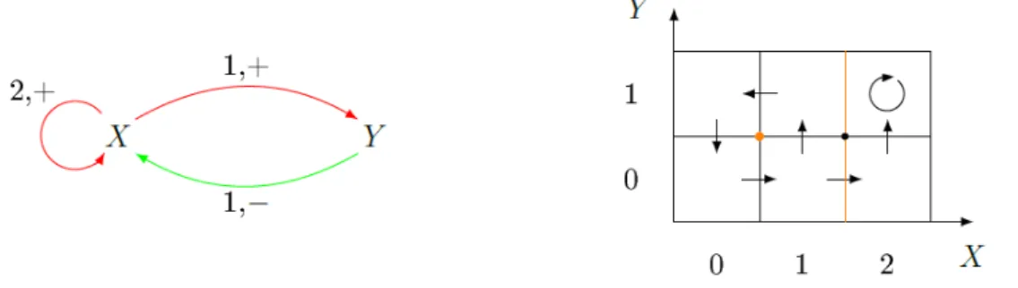
This work is part of one of those projects. The main idea is to utilise the characteristics of the combinatorial multivector fields to offer a different way to analyse the behaviour of genes and proteins, linking the mathematical structure to the gene regulatory networks. In fact a common method used to study the dynamics of these networks is Thomas’ formalism [10] which leads to the study of dynamics on cubical grids [11]. To give an idea to the reader, in Fig.3.1 is shown a representation of a gene regulatory network and

(39)

a transitive graph based on a structure which is similar to a cubical complex. In order to achieve the goal of the project, which is still under

develop-Figure 3.1: On the left, a representation of a gene regulatory network. The two genes, X, Y, encode proteins which have action on both genes. On the right, a graph which represents the dynamics of the gene regulatory network on the left.

ment, we want to offer an interactive way to scientists to query a database of combinatorial multivector fields, filtering the results and showing them in a proper way.

The algorithm showed in the previous section is needed to complete the first step of the project. In fact we needed to have all possible combinatorial mul-tivector fields on a 2 × 3 cubical complex. That is because associating the dynamics of a gene regulatory network to a combinatorial multivector field, we want to enable the user of our work to study all possible situations. That was a challenging problem due to the enormous quantity of data; we will present some numbers later in the section dedicated to the data and results.

As we wanted to allow whoever to modify every part of the whole project, we decided to use Python [7, 8] as main language due to the fact that it is more and more used for scientific computing; some of the main reasons are showed in [13].

(40)

3.2 Implementation of the algorithm 27

3.2 Implementation of the algorithm

As we said we decided to use Python as main language of the project. Although someone could argue about the efficiency of a script language for big computation problems, as said in [9] Python can be a reasonable alterna-tives to conventional languages such C or C++. Especially if we care about the readability of the code and we want to allow anyone, with some base knowledge, to understand and modify the code with respect to their needs.

3.2.1 Data Structures

Before seeing the two different implementations of our algorithm, we want to talk about the data structure we chose to represent our data, namely cubical complex and proper configuration.

Cubical complex

Between the two data types, the one used to represent a cubical complex is the only complex object.

We represented it with a custom Python class initialised by two integers representing the dimension of the grid. The initialization of the object creates some utility data used to increase the efficiency of the algorithm:

• An array dim which contains the dimension of every cell of the cubical complex i.e. dim[i] contains the dimension of the cell i. Obviously, the length of the array is equal to the dimension of the complex.

• A map neighbours which contains for every cell the list of cells to which it is possible to connect. For instance, every square has an empty list in the map because they cannot connect to any other elements.

Moreover the class has a static list of all the proper set in a 1 × 1 cubical complex. That list is used by the function which checks if a multivector is proper or not; we will talk about that function in the section dedicated to the multi-core version of the algorithm.

(41)

Proper configuration

It was a challenging problem to decide which structure to make use of to represent the configurations. That is because of the large amount of data produced both during the computation and during the storing of the output. Finally we decided to use a simple mono-dimensional array. It is easy to see that a grid is representable by a bi-dimensional array. A bi-dimensional array is easy to translate in a mono-dimensional array. That structure grants us enough ease of use and a small amount of memory usage/occupation. Therefore each configuration is written as an array of length equal to the dimension of the input cubical complex. Every entry of the array contains the index of the cell to which the element, represented by the entry, is connected. Note that every index of the array representing a square, will contain the index itself because the 2-cell can have an outbound connection just with itself. An example is shown in Fig. 3.2.

Figure 3.2: A proper configuration on a cubical complex 1 × 1 and its repre-sentation in our Python algorithm.

(42)

3.2 Implementation of the algorithm 29

3.2.2 Multi-core version

The first version developed, which is the one we used to compute the results, was a multi-core version. We develop this version to be used on the super computer of the faculty which has 120 cores.

Multiprocessing module

We chose to rely on the multiprocessing module which is part of the Python’s standard library. That is a powerful module similar to the thread-ing one but with some new APIs. Moreover usthread-ing sub-processes instead of threads it allows to fully exploit the power of the multi-core.

Among the structures in the multiprocessing package, we just used the class Process. Namely an object of that type represents an activity running in a separate process. Below an example is shown, taken from the official docu-mentation, of how to start a process, giving to it a function to compute. from m u l t i p r o c e s s i n g import P r o c e s s def f ( name ) : print ( ’ h e l l o ’ , name ) i f n a m e == ’ m a i n ’ : p = P r o c e s s ( t a r g e t=f , a r g s =( ’ bob ’ , ) ) p . s t a r t ( ) p . j o i n ( ) Parallel algorithm

The algorithm we designed is easily adaptable to a parallel version. The idea is straightforward, after reaching a certain level l of a PCTree with n nodes, we are ready to start n processes on each node. That is because each

(43)

branch is clearly independent of the others.

In particular in our implementation based on a cubical complex 2 × 3 we decided to visit the tree with one process until the level 10. At that point we have 7776 proper configurations, which are the nodes of the tree. Each process takes one node and computes the complete sub-tree up to the leaves. Once a process finishes its work, the main process will start another com-putation on one of the remaining nodes until there are no more nodes to analyse.

To manage the memory, when a process reaches a certain amount of proper configuration then it writes the list on a compressed file using the module gzip of the Python’s standard library. In that way, we are not only able to free the memory but we create a kind of checkpoint which in case of failure could prevent us to start again the computation from the beginning.

Proper set

An important part of algorithm is to check if a multivector is proper or not. That operation is done for every multivector of every configuration analysed, which means a huge amount of time.

We developed a specific method which is able to verify if a configuration is proper or not in linear time in the number of components of the graph. The method is specific because it works just on the cubical complex we are working with.

The idea is that we can consider a 1 × 1 cubical complex as our base unit. Every n × m cubical complex is made by n · m units. It is easy to see, as they are the same, that every unit can have the same proper sets. In other words if a set is improper (proper) on one of the squares, moving the set on another square but on the same position does not change the fact that the set is improper (proper), as shown in Fig. 3.3.

Therefore given the list of all possible proper sets containing a square in a cubical complex 1 × 1, which has a fixed size of 47, our method checks if a configuration is proper or not by taking each component, shifting its indexes

(44)

3.2 Implementation of the algorithm 31 to the relative ones in a 1 × 1 cubical complex and checking the list.

The Python function below shows how to shift the indexes of a multivector. In the function we use the following variables and functions:

• c, represents the cubical complex which the multivector belongs to. • square, represents the index of the square in the multivector. We know

we can have just one square in a multivector. We also know that a set cannot be improper without a square.

• mv, represents the multivector we want to check. • db, dc, are parameters used for the shifting. • c.xCells, identifies the number of cells per line.

• c.row(i), returns the index of the row to which the i-cell belongs. To do that we just apply a simple formula c.row(i) = bi/c.xCellsc. def s h i f t I n d e x e s ( c , s q u a r e , mv ) : db = c . x C e l l s + 1 − 4 dc = s q u a r e − 4 squareRow = c . row ( s q u a r e ) mvTrasl = [ ] f o r i in mv : s h i f t e d I n d e x = i + ( squareRow−c . row ( i ) ) ∗ db − dc ) mvTrasl . append ( s h i f t e d I n d e x ) return mvTrasl

3.2.3 Distributed version

The enormous quantity of managed data requires appropriate computa-tional resources. In particular, as we will discuss in the last section, our machine was able to compute the combinatorial multivector fields on a cu-bical complex 3 × 2, which was what we needed, but will not be enough in

(45)

Figure 3.3: On the left, a cubical complex 1 × 1 with a proper set P = {0, 3} and an improper set IP = {4, 7, 8}. On the right, a cubical complex 1 × 2 in which we move both P and IP on the two squares. Obviously the sets remain proper, respectively improper.

case of bigger structure.

Therefore, with an eye to the future, we wanted to allow even bigger com-putations taking advantage of a distributed computing. To do that we chose to use the Spark engine [14, 15] together with the hadoop distributed file system (HDFS) [16, 17].

Hadoop distributed file system

HDFS is the distributed file system provided by Hadoop [18]. It has a master-slave architecture. An HDFS cluster consists of a single namenode, the master, and a number of datanodes. The namenode executes file system namespace operations while the datanodes are responsible for serving read and write requests from the file systems clients. Internally, a file is split into one or more blocks and these blocks are stored in a set of datanodes.

We chose to utilize HDFS mainly because Spark has some APIs to easily interact with the distributed file system.

We configured HDFS to be used in a pseudo-distributed way. Namely we start the file system on a single node, simulating datanodes with separate

(46)

3.2 Implementation of the algorithm 33 Java processes. To configure HDFS in order to work in that way we modified two configuration files in the following way:

/hadoop directory/etc/hadoop/core-site.xml <c o n f i g u r a t i o n> <p r o p e r t y> <name> f s . d e f a u l t F S</name> <v a l u e> h d f s : // l o c a l h o s t : 9 0 0 0</ v a l u e> </ p r o p e r t y> </ c o n f i g u r a t i o n> /hadoop directory/etc/hadoop/hdfs-site.xml.xml <c o n f i g u r a t i o n> <p r o p e r t y> <name>d f s . r e p l i c a t i o n</name> <v a l u e>1</ v a l u e> </ p r o p e r t y> </ c o n f i g u r a t i o n> Spark

Spark is an open-source framework used for processing big data. It of-fers high-level APIs in the following programming languages: Java, Scala, Python and R. Thanks to its performance, it is more and more considered as the best tool for general-purpose data processing.

To achieve these performances Spark introduce a distribute memory abstrac-tion called Resilient Distributed Datasets (RDDs) [19]. These objects allow the programmers to perform in-memory computations on large clusters in a fault-tolerant way.

Talking about the configurations, Spark comes out with a build which al-ready includes a linking to hadoop. We just had to tune some parameters

(47)

editing the file /spark directory/conf/spark defaults.conf. In the list below we explain the purpose of these parameters giving an example for each of them.

• spark.driver.memory 1g

It sets the maximum amount of memory the driver can use. The driver is the master, therefore it does not usually need lot of memory.

• spark.executor.memory 2g

It sets the maximum amount of memory the executor can use. As executor we mean a worker. In our case, with respect to the size of the cubical complex, the executors need to consume a big amount of memory.

• spark.network.timeout 600s

It sets the timeout time for the network operation i.e. mostly, in our case, when the driver has to collect data from the executors.

Distributed Algorithm

As we said, Spark allows to write code in Python. In particular it offers a Python interactive console. As we want to enable anyone to use the produced data in an interactive way, we chose to develop for that console.

The only change to the algorithm we had to make is a transformation from a recursive version to an iterative one, finally introducing some Spark prim-itives.

To use our algorithm, once we started the interactive console with the fol-lowing instruction

./spark directory/bin/pyspark

and we included our code, it is possible to call the function generateCMF( sc, n, m, monoProcLimit) where

(48)

3.3 Data and results 35 • sc is the Spark context. In pyspark, the variable is exactly called ’sc’. • n,m represent the size of the cubical complex.

• monoProcLimit indicates how many cells a single core has to analyse before starting the parallel computation.

3.3 Data and results

In the current section we want to show you some interesting data and information about our tests and the final results.

It still is a challenging problem to try to estimate the time needed by our algorithm related to the size of the analysed cubical complex. That is for various reasons. First of all we do not know a priori how many combinatorial multivector fields we have. Moreover it was rather hard to execute some tests because of the long processing time required and the memory consumption.

3.3.1 Estimate resources consumption

In order to try to estimate the total time needed for the processing, we decided to execute the algorithm limiting the number of branch analysed after the mono-process execution.

For our experiments we used the machine described below

Model name: Intel(R) Core(TM) i7-6700HQ CPU @ 2.60GHz CPU(s): 8

RAM: 16gb

and the parameters shown in Table 3.1.

The time needed for a single process to compute the first 10 branches of the PCTree is negligible. Then we decided to start the computation on 5 cores,

(49)

Table 3.1: Parameters of our tests for the estimation of the performances. choosing randomly 5 branches.

The graphs in Fig.3.4 and Fig.3.5 show tests’ result.

Taking the average values of those experiments, we estimated that the aver-age processing time for a branch is of about 1773 seconds with a disk usaver-age of 3,05GB per branch. Therefore multiplying the obtained values by the number of branches we have

Total estimated processing time: 160 days Total estimated disk required: 23.7 TB

Obviously the time is considered for mono-process computation. Therefore, considering the machine we had for the final computation which is described below

Model name: Intel(R) Xeon(R) CPU E7-8867 v3 @ 2.50GHz CPU(s): 120

RAM: 1TB

we can divide the estimated processing time by the cores number, obtaining an estimated time of 31 hours.

(50)

3.3 Data and results 37 Thanks to the estimated disk usage, we supposed to generate about 220.000.000.000 proper configurations.

Figure 3.4: Time performance during the 5 experiments. Time on the y-axis is expressed in seconds.

Although the method used to estimate the resources consumption, above described, is clearly not accurate, to the best of our knowledge this is the most suitable testing procedure.

3.3.2 Results

In this kind of work there is not so much information to give about the results we obtained. It will clearly be more interesting to analyse, at the

(51)

Figure 3.5: Size of the results obtained during the 5 experiments. Size on the y-axis is expressed in gigabytes

second step of the project, the query time and how to improve the perfor-mances.

Nevertheless we want to show you some data and compare it with the esti-mated one.

We finally generated 199.246.400.336 proper configuration on a cubical com-plex 2 × 3, with 2,2 days of computation and 22TB of files generated. Even though the method utilised for the test is not that reliable, the results we estimated are not so far from the real ones.

A separate discourse needs to be entered into for the processing time. First of all the experiments and the final computation were executed on different machines. That fact does not change the results about the size and quan-tity of data generated, but it clearly influences the time needed to compute.

(52)

3.3 Data and results 39 Moreover we observed a problem with the RAM, most of which were used by the buffer cache of the operating system, that logically slows down the performance.

We were not able to test the distributed algorithm on the 2 × 3 cubical com-plex, because the software needed for the implementation was not available on that machine. Therefore we limit out experiments, using that algorithm, on a cubical complex 2 × 2 comparing the time performance with the par-allel algorithm on the same data structure. We noted that the distributed algorithm is able to compute all the data on that structure using half of the time of the parallel one. Note that, since Spark was configured as pseudo-distributed, both algorithms could be considered parallel and the increment of performance has to be considered to be related just to the difference be-tween Spark and the Python multiprocessing’s module.

(53)

(54)

Conclusions

The aim of this dissertation was to design, validate and develop an algo-rithm for the generation of all possible combinatorial multivector fields on cubical complexes. That is the first step of a project, carried on by a group of researchers of the Faculty of Mathematics and Computer Science at the Jagiellonian University of Krakow, which aims to allow to study the dynam-ics of gene regulatory network using that topology structure.

We designed a method together with a formal mathematical proof, which let us generate in a reasonable time, using the supercomputer of the Faculty, around 200 billions structures.

We provided two different implementations using Python as programming language and Spark, together with Hadoop HDFS, for a distributed compu-tation.

We are really satisfied with the results, because they allowed the researchers to work with much more complex gene networks than previously. Moreover the results obtained on the test of the distributed version show that it will hopefully be possible to compute even bigger data structures.

Talking about the future, there still are several works to be done.

First of all, the distributed algorithm needs to be tested on a real distributed context and with bigger data. In particular the method has to be adapted in order to allow a checkpoints system as in the parallel computation. We were not able to test the second version of the algorithm on bigger complex because the supercomputer have not Spark and HDFS.

Finally, the rest of the whole project needs to be developed. Namely using 41

(55)

the interactive Python console on Spark, we have to allow the user to query and filter the enormous database of combinatorial multivector fields, provid-ing appropriate output.

(56)

Bibliography

[1] Mrozek, Marian. ”ConleyMorseForman Theory for Combinatorial Mul-tivector Fields on Lefschetz Complexes.” Foundations of Computational Mathematics (2016): 1-49.

[2] Edelsbrunner, Herbert, and John Harer. Computational topology: an introduction. American Mathematical Soc., 2010.

[3] Lefschetz, Solomon. Algebraic topology. Vol. 27. American Mathemati-cal Soc., 1942.

[4] Kaczynski, Tomasz, Konstantin Mischaikow, and Marian Mrozek. Com-putational homology. Vol. 157. Springer Science & Business Media, 2006. [5] Mrozek, Marian, and Thomas Wanner. ”Coreduction homology algo-rithm for inclusions and persistent homology.” Computers & Mathe-matics with Applications 60.10 (2010): 2812-2833.

[6] Queyranne, Maurice, and Laurence Wolsey. ”Modeling Poset Convex Subsets.” CTW. 2015.

[7] ”Python 3.5.3 documentation”. https://docs.python.org/3.5/. Last Ac-cessed 4 February, 2017.

[8] Pilgrim, Mark, and Simon Willison. Dive Into Python 3. Vol. 2. Apress, 2009.

[9] Prechelt, Lutz. ”An empirical comparison of C, C++, Java, Perl, Python, Rexx and Tcl.” IEEE Computer 33.10 (2000): 23-29.

(57)

[10] Snoussi, El Houssine, and Rene Thomas. ”Logical identification of all steady states: the concept of feedback loop characteristic states.” Bul-letin of Mathematical Biology 55.5 (1993): 973-991.

[11] Bernot, Gilles, et al. ”Application of formal methods to biological regu-latory networks: extending Thomas asynchronous logical approach with temporal logic.” Journal of theoretical biology 229.3 (2004): 339-347. [12] Bush, Justin, et al. ”Combinatorial-topological framework for the

anal-ysis of global dynamics.” Chaos: An Interdisciplinary Journal of Non-linear Science 22.4 (2012): 047508.

[13] Oliphant, Travis E. ”Python for scientific computing.” Computing in Science & Engineering 9.3 (2007).

[14] ”Apache Spark: Lightning-fast cluster computing.” http://spark.apache.org/. Last Accessed 2 September, 2017.

[15] Zaharia, Matei, et al. ”Spark: Cluster computing with working sets.” HotCloud 10.10-10 (2010): 95.

[16] Shvachko, Konstantin, et al. ”The hadoop distributed file system.” Mass storage systems and technologies (MSST), 2010 IEEE 26th symposium on. IEEE, 2010.

[17] ”HDFS Architecture Guide.” https://hadoop.apache.org/docs/r1.2.1/hdfs design.html. Last Accessed 2 September, 2017.

[18] ”Welcome to Apache Hadoop!.” http://hadoop.apache.org/. Last Ac-cessed 2 September, 2017.

[19] Zaharia, Matei, et al. ”Resilient distributed datasets: A fault-tolerant abstraction for in-memory cluster computing.” Proceedings of the 9th USENIX conference on Networked Systems Design and Implementation. USENIX Association, 2012.

(58)

Acknowledgements

I would like to thank my Polish supervisor Mateusz Juda because he was always ready to help me during my stay in Krakow.

I would also like to thank all my Erasmus friends who spent time with me during the best experience of my life and somehow helped me to finish this work.

(59)

(60)

Ringraziamenti

Vorrei ringraziare il Prof. Massimo Ferri sopratutto perch´e mi ha per-messo di partecipare al progetto Erasmus a Cracovia e vivere una fantastica esperienza, senza dimenticare il supporto continuo fino ad oggi.

Vorrei ringraziare il Prof. Giulio Casciola per la sua immensa disponi-bilit`a.

Vorrei ringraziare tutti gli amici di Bologna, se è andata come è andata è anche merito loro.

Banale ma dovuto, ringrazio la mia famiglia a cui dedico completamente questo lavoro.

An algorithm for the generation of all possible combinatorial multivector fields on cubical complexes