Chain entanglements and fracture energy in interfaces between immiscible polymers

(1)

Tesi

presentata a conclusione del corso di perfezionamento in “Scienze Dei Materiali” finanziato dalla societ`a Mapei S.p.A.

Chain entanglements and fracture energy in

interfaces between immiscible polymers

Leonardo Silvestri

Supervisors: Chiar.

mo

Prof. Franco Bassani

Chiar.

mo

_{Prof. Sergio Carr`a}

(2)

(3)

Abstract

Entanglements are the ultimate source of toughness in glassy polymers, in fact at molecular weights lower than the critical molecular weight for entanglements they become quite brittle. Similarly, the strength of an interface between two immiscible glassy polymers is determined by the density of entangled strands that cross it, usually denoted by Σeff. This is a microscopic quantity that cannot be measured or

controlled directly, except in very special cases, and therefore it is important to relate it to some significative macroscopic parameter characterizing the interface. In recent years many experimental works proved that there is a clear correlation between the toughness of an interface between glassy polymers and its width, so that models of entanglements at interfaces have become necessary to interpret the data. Some theoretical approaches have been proposed in the last few years, but their agreement with experimental data cannot be considered completely satisfactory.

In this thesis we propose a new model to describe entanglements at interfaces, that relates the fracture energy of an interface between immiscible polymers to its width [1]. The role of other important parameters, first of all the molecular weight of the polymers, is also investigated.

The starting point is a study of the interfaces between immiscible polymers at thermodynamical equilibrium. To this end we use a Self Consistent Field approach, which is suitable for the strong and intermediate segregation regime, to numerically derive concentration profiles and mean fields.

The central part of this work is devoted to the calculation of Σeff, with a method,

(4)

approach successfully applied by Mikos and Peppas [2] to symmetric interfaces. Nu-merical results are obtained using the Self Consistent mean fields and the dependence of Σeff on the interface width and polymers molecular weights is shown. Following

previous literature descriptions, possible fracture mechanisms, depending on the values of Σeff, are then discussed and a new fracture regime is introduced, called

“partial crazing”, to account for the intermediate situation in which a craze starts in one of the two materials but it cannot fully develop. Numerical results for the fracture energy as a function of interface width and polymers molecular weights are compared with literature experimental data, showing good agreement. In the case of PMMA/P(S-r-MMA) interfaces, the dependence of the fracture energy on the interfacial width could be reproduced very well over the whole range of investigated widths, more satisfactory than in previous literature works.

The last chapter of this work is focused on the calculation of the molecular weight of entanglements Me, which influences greatly the value of Σeff. This quantity has

been measured in bulk polymers, but, to our knowledge, never at a polymer-polymer interface. Moreover, theories that clarify the nature of entanglements and allow speculations on the value of Me in inhomogeneous systems, have been proposed only recently. In this work the packing model for entanglements is adopted to estimate the value of Me at polymer-polymer interfaces and in thin polymer films. Our numerical results show that the molecular weight of entanglement of chains near an interface is larger than in the bulk, leading to appreciable corrections in the Σeff

and fracture energy calculations. We also compute the average molecular weight of entanglements in thin films, and predict that it should increase as the thickness of the film decreases below the entanglement length.

(5)

Acknowledgements

This Ph.D Thesis concludes a three years research at the Scuola Normale Superiore in Pisa financially supported by MAPEI S.p.A., that the author wishes to thank.

There are a number of people who assisted in preparation of this thesis. First of all I wish to thank my supervisors, Prof. Franco Bassani and Prof. Sergio Carr`a, who have been a constant source of encouragement and guidance throughout my whole Ph.D studies. Thanks also goes to Stefano Carr`a for his precious suggestions and for being always ready to offer his help in both scientific and everyday matters. I’m also grateful to Prof. Hugh Brown, with whom I have had the pleasure of collaborating at the University of Wollongong. I will never be able to thank him enough for the time he has dedicated to me and for the enlightening discussions we had. I would also like to thank Robert Oslanec for his help with the numerical calculations and for sharing with me his computer programs.

This work wouldn’t have been possible without the support of my family, who backed me during the frantic days of its preparation.

The final lines are for Camelia, who listened to my endless talking about polymers and spent her summer days checking the final manuscript with me. To her this thesis is dedicated.

(6)

(7)

Chapter 1 Introduction

The adhesion of polymers is relevant in many scientific and technological areas and has become in recent years a very important field of study [3]-[7]. Its main applica-tion is bonding by adhesives, but adhesion is also involved whenever two polymers are brought into contact, as in coatings, paints, polymer blends, filled polymers or composite materials. Even the toughness of a bulk polymer, for example, can be viewed as a problem of adhesion between two pieces of the same material. In general the final performance of these materials depends significantly on the quality of the interfaces formed inside them; it is therefore understandable that a better knowledge of adhesion is very important for many practical applications. Yet only 50 years ago adhesion became a scientific subject in its own right. The reason is probably that the understanding of adhesion requires a knowledge in many different fields, ranging from macromolecular science and physical chemistry of surfaces and interfaces to materials science, mechanics and rheology. It is well known for example that adhe-sive properties of polymeric materials rely not only on the strength of interfaces they can form, that have to sustain the stress, but most of all on their ability to dissipate energy in the bulk. A full comprehension of both aspects of the problem involves then many different research fields, as we will see for glassy polymers systems.

The first subtle question that needs to be answered when studying this subject is probably how toughness is measured. In fact it is not obvious what is the best physical quantity to characterize the strength of an interface. One could say that it

(10)

is the maximum stress that the interface can sustain, called “fracture strength”, but this is not the best choice. In real systems there are always flaws and cracks leading to values of the local stress much higher than the average applied stress. The result is that interfaces usually fail much earlier than expected. A more useful approach is to invoke an energy criterion: an interface fails if a pre-existing crack can grow. This happens when the strain energy released by the failure of the interface is greater than the energy needed to create two new surfaces. The strength of an interface in practical cases is therefore related to the latter quantity, that is called “fracture energy” and is indicated with Gc.

The problem that we face now is how to estimate Gc for glassy polymers. If we could separate two surfaces A and B in a thermodynamically reversible way, then the fracture energy would be equal to the work of adhesion WAB = σA+ σB− σAB, where σA and σB are the surface tensions and σAB is the interfacial tension. For an interface between two identical material the above formula gives a work of cohesion of twice the surface tension. With such an approach we would obtain for glassy polymers a fracture energy of about 0.1 J/m2_{[8], while measured fracture energies of}

many glassy polymers reach values four order of magnitude higher and are strongly dependent on the polymer molecular weight [9]-[12]. In particular a transition is observed at molecular weights close to the critical molecular weight for entanglement

Mc, after which the fracture energy increases abruptly and then reaches a plateau at infinite molecular weight, as shown in Figure 1.1. High fracture energies are also known to be associated with the intermediate formation of a craze, that is a plastic deformation, localized around the crack zone, capable of dissipating a great amount of energy [13]-[15]. These experimental observations make it immediately clear that entangled chains are essential to improve cohesion and to obtain crazing in the bulk; nevertheless a quantitative explanation of the experimental results has not been achieved for many years.

It is easy to imagine that, when trying to propagate a crack inside a glassy polymer, all the chains that are entangled at both sides of the crack will oppose some resistance. Such a chain coupling across the interface can be described by the areal density of entangled strands that cross it, indicated by Σeff, which is

(11)

3

Figure 1.1: Fracture energy G1cversus molecular weight, for PS in the virgin state. The fracture energy starts to increase very quickly at Mc ≈ 32000, and reaches a plateau at M ≈ 8Mc. After R.P. Wool [6].

proportional to the maximum stress an interface can withstand. For symmetric interfaces a simple model, similar to Lake and Thomas theory of elastomers [16], predicts Σeff = ρeLe/2 , where ρe is the density of entanglements and Le is the root mean square end to end distance between them [13]. Such an expression is correct in the limit of infinite molecular weights, but can not explain the molecular weight dependence of the fracture strength found experimentally. A more accurate expression was derived by Mikos and Peppas [2], who used a stochastic approach to count the number of coupling strands across a fracture plane in bulk polymers and included chain end effects in their analysis. They subdivided each chain in segments of Ne monomers and assumed that each of them formed an entanglement, except the first and last ones. In this way they could take into account the fact that dangling ends do not contribute to entanglements, and predicted that the infinite molecular weight Σeff should be scaled by a factor 1 − 2Me/M. This agrees with the normalized experimental data and with the observation that usually Mc≈ 2Me. Yet

(12)

the connection between Σeff and the fracture energy still posed problems, because

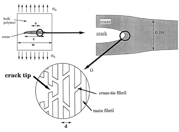
of the difficulties in describing crazing. Crazed material was believed to be made of parallel load-bearing fibrils running perpendicularly to the interface, so that any theory predicted a fracture energy proportional to Σeff. The problem was that, in

order to reproduce experimental results, the energy needed to break C-C bonds should have been one order of magnitude higher than the measured values. The solution was found by Brown [17], who first recognized the importance of the cross-tie fibrils that connects primary fibrils and are capable of transferring load. He modelled the craze as an elastic continuum and computed the stress amplification at the crack tip, demonstrating that Gc ∝ Σ2eff, as described in detail in section

3.3. This scaling law has been confirmed since then by a number of experiments performed on interfaces reinforced by block copolymers, and could finally explain the high fracture energies of glassy polymers. A summary of the mentioned experimental data is presented in Figure 1.2, while experimental details are discussed further down in this section.

In technology the use of pure materials is rare, because usually people need to combine in a single mixture the properties of different materials. Unfortunately, in the absence of specific interactions, most of polymers are immiscible so that in mixing them you end up with a number of coarse domains of the pure materials. Moreover the interfaces between such domains are very weak, with the result that the final composite material is useless. For these reasons a knowledge of the interfacial properties is often very important from a technological point of view.

The starting point of any study of the strength of an interface is a knowledge of the equilibrium properties of the interphase between them, and the most interesting quantity to know is probably the degree of interpenetration between species, or in other words the concentration profiles. The two general theoretical approaches for describing interfacial properties of polymer system are based on Self Consistent Field (SCF) [18]-[29] and Density Functional methods [30]-[39]. The latter approach consists in writing the free energy of an inhomogeneous system as a functional of the unknown densities, that are then found by minimization of such a free energy. The free energy functional is generally written as a functional expansion around the

(13)

5

Figure 1.2: Fracture energy of interfaces reinforced with block copolymers as a function of the effective areal density of chains crossing the interface. Triangles and squares are for polystyrene/poly(2-vinyl pyridine) interfaces reinforced with styrene-2-vinyl pyridine block copolymers [56]. Circles are for poly(xylenyl ether)/poly(methyl methacrylate) interfaces reinforced with styrene-methyl methacrylate block copolymers [17],[57]. After Creton et al. [56].

homogeneous blend expression. Due to its nature this method is appropriate only for weakly immiscible polymer pairs and wide interfaces, when the square gradient term alone is sufficient, but it has the great advantage that analytical results can be often obtained. Self Consistent Field approaches require instead computer intensive calculations, but can also be used in the intermediate and strong segregation regimes. The SCF method is the one we adopted and will be described in detail in chapter 2; we only recall here briefly recall how this method works. Mean fields are expressed as functionals of the densities, that in turn can be computed from a probability density satisfying a modified diffusion equation with a potential term given by the above mean fields. The corresponding coupled equations for fields and densities are then solved numerically by a self-consistent algorithm.

(14)

incom-pressible Flory-Huggins expression for the homogeneous polymer blend [3], that is sufficiently detailed for our study of the interface toughness. However it is worth mentioning that more sophisticated expressions are available, to include the effects of compressibility, specific interactions, block copolymers, grafted chains, etc.. [40]-[41]. An interesting improvement in this sense is the Lattice Cluster Theory (LCT) by Dudowicz and Freed [41]. It is a lattice based model, where monomers are allowed to occupy more than one site and to have different structures, while compressibility is taken into account by adding voids as non-interacting particles occupying only one site. Corrections to the mean field approximation are then systematically added to the free energy expression through a double power expansion in the microscopic interaction energies and in the inverse lattice coordination number. With this ap-proach Freed and coworkers could explain effects due to monomer structures, as the temperature independent term in the effective interaction parameter χ, that is due to non-combinatorial entropy of mixing, or the miscibility of polyolefin blends [42]. The theories described above have been extensively tested against experimental results for interfacial widths and tensions, displaying a good agreement within their range of validity [43]-[49].

The toughness of interfaces between immiscible polymers instead has started to be investigated only recently, raising new questions about the concept of entan-glement. The typical experiments on these systems are set up as follows. Two immiscible glassy polymers are annealed at a temperature T above the glass tran-sition temperatures, Tg, of the two species, for a time that is long enough to reach thermodynamical equilibrium. Then the system is cooled down very quickly to room temperature and the fracture energy of the glassy joint is measured. This measure-ment is usually performed by an asymmetric double cantilever beam test, in which two welded polymer bars of different thicknesses are driven apart by a razor blade of known width, as illustrated in Figure 1.3. The length of the crack ahead of the blade is then measured and the fracture energy is computed from the known geometric and elastic properties of the beams. In such experiments the ratio of bar thicknesses is chosen to obtain the smallest value of the fracture energy; in this situation the crack propagates at the interface and the applied stress is purely tensile. The

(15)

cor-7

responding fracture is usually referred to as mode I, and the corresponding energy is sometimes indicated with GIc. Mode I failure gives the lowest values of fracture

energy and it is also better understood from a theoretical point of view. These ex-periments have been performed for a range of different materials and experimental conditions [50]-[58], so that some data are now available in the literature, allowing theoretical models to be tested.

Figure 1.3: Asymmetric Double Cantilever Beam Test. The arrangement is asymmetric to compensate for differences in elastic and crazing properties between the two materials, as discussed in the text. After Creton et al. [56].

The first conclusion that can be drawn is that entanglements are essential in strengthening the interfaces between immiscible polymers. Many experimental groups have measured, for instance, the interfacial fracture energy between polystyrene (PS) and poly(methyl methacrylate) (PMMA) finding values between 10 and 20 J/m2

[50]-[52], much less than bulk fracture energy of both polymers, but substantially greater than the ideal work of adhesion. Moreover they found that, similarly to what happens in bulk glassy polymers, at low molecular weights, Gc drops below 3 J/m2 _{[52]. A qualitative explanation of such results is not difficult: the extent}

of entanglement is much smaller in interfaces than in the bulk. In fact the inter-face between PS and PMMA has a width of only 3 nm, while the distance between entanglements in polystyrene is about three times greater.

(16)

Figure 1.4: Schematic of a layer of A-B block copolymer chains segregated at a A/B interface. After Creton et al. [56].

chain coupling across the interface by Σeff, which is also the quantity determining the

failure mechanism. Important information about this aspect can be obtained from experiments on interfaces reinforced with block copolymers. We know that when a diblock copolymer AB is placed at an A/B interface, each block will mix with its homopolymer, as shown schematically in Figure 1.4. It is then possible to assume that all the copolymer chains will cross the interface, and to compute the contribute to Σeff due to the copolymer from its density. Moreover for strongly immiscible

pairs the homopolymer contribution can be neglected, so that for such systems Σeff is perfectly known. Creton et al. [56] studied an interface between PS and

poly(2-vinylpiridine) (PVP) reinforced with block copolymers of PS and PVP. They showed that different failure mechanisms occur depending on the molecular weight of the blocks and on Σeff. Short blocks, that are not long enough to be entangled

with their homopolymers, can be easily pulled out from their surroundings and only small increases of fracture energy can be obtained. At higher molecular weights, i.e. when M > Mc, and low Σeff, the active failure mechanism is chain scission,

as proved by surface analysis that measured the fraction of blocks on each side of the interface after failure. At high molecular weights and high Σeff, crazing is the

(17)

9

preferred mechanism and fracture energies are very high. Similar conclusions were confirmed also by Dai et al. [58], who investigated the same system with similar techniques, and by Creton et al. [59] who studied interfaces between PMMA and poly(phenylene oxide) (PPO) homopolymers reinforced with varying amounts of a PMMA-PS block copolymer. A useful picture of the transition between different failure modes is given in Figure 1.5, where we report experimental results from Kramer [60], showing how the fracture mechanism changes from chain scission, in which Gc∝ Σeff, to crazing, in which Gc ∝ Σ2eff, when Σeff increases.

Figure 1.5: Reinforcement of a PS/poly(vinyl pyridine) interface by a deuterated styrene (dPS)-vinyl pyridine block copolymer. Circles (right-hand axes) show the measured frac-ture energy, and crosses the fraction of dPS found on the PS side of the interface after fracture, both as a function of the copolymer chain density. The discontinuity of the curves at Σ = 0.03 nm−2 indicates a transition from chain scission to crazing. After Kramer et al. [60].

(18)

toughness of an interface, but in non reinforced systems Σeff cannot be measured.

It would be therefore desirable to link it to measurable parameters of the interface. We can start from the observation we made on PS/PMMA systems: if the width is much lower than the distance between entanglements then they are not very effective in reinforcing the interface. This simple prediction has been investigated in some recent experiments. Schnell et al. [53] measured the fracture energy of bilayers of PS and poly(para-methyl styrene) (PpMS), for a wide range of interfacial widths, obtained by changing the annealing temperature of the samples. In this way, they were able to demonstrate that there is a clear correlation between the width, measured by neutron reflectivity, and the fracture energy of the interface. The results were confirmed in another work of the same authors on interfaces between PS and the statistical copolymer of poly(bromostyrene-styrene)(PBrxS) [54]. The same correlation has been found by Brown [55], who measured the toughness of the interface between a random copolymer P(S-r-PMMA) and pure PMMA, for different fractions of PS in the copolymer. In order to show how Gcdepends on the interfacial width, we reproduce in Figure 1.6 a plot in which several experimental results are reported together.

It would be of great importance to establish a quantitative relation between width and toughness, because it would allow easier predictions of the strength of interfaces and would clarify the concept of entanglement. For weakly immiscible polymer pairs, De Gennes [61] proposed a scaling law for the dependence of Σeff on

the interface width through the Flory-Huggins interaction parameter χ. However, his result is based on energetic considerations, and it does not take into account properly the effect of inhomogeneous polymer densities at the interface. In recent years a new approach has been proposed by Brown [55], in which Σeff depends

only on the concentration profile of the polymer. He assumed that the probability that a strand starting from x might end in x0 _{is proportional to the ratio of the} polymer volume fractions at the two points, but we will see in chapter 3 that this is not correct. As a result, his model predicts a variation of the density of effective entangled chains that is too slow with respect to the changes in the interface width. Both models are discussed in detail in section 3.2.

(19)

11

Figure 1.6: Fracture energy Gc plotted as a function of the interfacial width aI for different samples: PS-PBrxS (open squares) [54], PMMA (filled squares) [44][50], PS-PpMS (filled circles) [53], and PS-PS (open circles) [53]. After Schnell et al. [54].

More generally, we believe that the main limitation of all available descriptions of the strength of interfaces is the scarce knowledge of entanglements. A great step forward in this direction has been done in the last fifteen years, when some new models have been proposed to link the molecular weight of entanglements to conformational characteristics of the polymer chains [62]-[69]. Recent experiments [67],[70] seem to confirm the validity of a particular the so called “packing models” for bulk glassy polymers, and some authors have already attempted to apply the same concepts to entanglements at interfaces and surfaces [71]-[73]. Unfortunately it is not clear how to determine experimentally the molecular weight of entanglement in interfaces, so that for these systems the predictions of different models cannot be tested. A possible way of measuring Me in thin films has been instead proposed by Brown and Russell [71], and experiments are currently being performed.

(20)

account for the experimentally found dependence of the toughness on the interfacial width. The work is organized as follows. In chapter 2 we study the thermodynamics of polymer blends, describing in detail the Self Consistent Field (SCF) approach and the numerical calculations we performed to obtain concentration profiles and mean fields at polymer-polymer interfaces. In chapter 3 a new model is presented that allows to compute the density of entangled strands across the interface. Our model, supplemented with an appropriate description of the fracture mechanisms and the introduction of a new fracture regime, describes very well the available experimental data. In particular it reproduces very well the dependence of the toughness on the interface width over the whole range of experimental widths. In the final part of this work, chapter 4, we adopt a packing model for entanglements and apply it to inhomogeneous systems in order to estimate Me. Numerical results show that the molecular weight of entanglement of chains near an interface is larger than in the bulk, and the corrections to the fracture energy calculations due to this effect are discussed. We compute also the average molecular weight of entanglements in thin films, showing how it increases as the thickness of the film decreases below the entanglement length. Conclusions and ideas for future developments are the subject of chapter 5.

(21)

Chapter 2 Self Consistent Field method for

polymer interfaces

The main goal of this work is to predict the strength of a joint as a function of its interfacial properties, and it is therefore natural to start from the thermodynamics of polymer mixtures. In particular we are interested in the equilibrium concentration profiles of the two joined polymers and in the mean fields that chains experience at the interface. As we will see in chapter 3 our model of entanglements is in fact based on a mean field approximation.

As already pointed out in the introduction two methods are commonly used to study inhomogeneous systems, that have different ranges of validity. Density Functional methods [30]-[39] can give some accurate analytic predictions for wide interfaces, but they are not very useful in the case of the strongly immiscible systems we want to study. A Self Consistent Field approach [18]-[29] is more suitable for strong and intermediate segregation and, even if it requires computer intensive cal-culations, it allows to compute at the same time the densities and the corresponding mean fields. For these reasons we will adopt a SCF method to obtain the needed equilibrium properties of interfaces.

The origins of the SCF approach can be dated back to the mid-1960s, when Ed-wards pointed out the analogy between the classical problem of interacting electrons and the “new” problem of interacting polymers [74]. Many methods were available at the time to deal with many body systems and they proved immediately

(22)

success-ful when first applied to polymers by Helfand and Tagami [18]. The problem was initially presented from a mean field point of view and only later a more comprehen-sive theory, based on a functional integral approach, showed the connection between that intuition and fundamental statistical mechanics [20]. In his works Helfand studied in detail the interface between two immiscible polymers that he assumed incompressible, and soon recognized the importance of avoiding fluctuations of the overall density. He therefore added to the free energy an “ad hoc” term proportional to the square of the deviation from the average density and to the inverse of bulk compressibility, to restrict such fluctuations. Some years later Hong and Noolandi [24] developed instead a truly compressible theory, that was derived from an earlier work on incompressible multi component polymer systems [23], by simply assuming one of the small molecule components to be vacancies.

We performed SCF calculations on interfaces with both methods and checked that, in the incompressible limit, they give the same results within the numerical errors. For convenience however we adopted the approach by Helfand [20], and followed the work by Shull et al. [25]-[28] to perform numerical calculations.

In this section we first derive correct SCF equations for inhomogeneous polymer systems following the work by Hong and Noolandi [23], and then describe in detail how we solved them in the case of interfaces, paying particular emphasis on the approximations of Helfand’s approach. We hope in this way to give a clear picture of the physics involved.

2.1 SCF equations for inhomogeneous polymer

sys-tems

The index p = 1, 2, ..., n labels the polymeric species, while we will indicate with the subscript 0 the voids. Summations involving also the vacancies will be denoted with the index k = 0, 1, ..., n. In this section, for consistency with the work of Hong and Noolandi [23], the number of chains of type p is denoted by ˜Np = Np/Zp, where

Np is the number of monomer units and Zp is the degree of polymerization. Of course Z0 = 1, so that we will use either N0 or ˜N0. Moreover we will assume that

(23)

2.1. SCF equations for inhomogeneous polymer systems 15

each vacancy occupies the same volume, that we will call υ and that can be in fact regarded as the lattice cell volume.

Our derivation starts from the grand partition function for a system with fixed number of particles, but a variable number of vacancies

Z =  Y k ZN˜k k ˜ Nk!   Z  YN0 i=1 δr0i(·)    Y p ˜ Np Y i=1 δrpi(·)P [rpi(·)]  _{exp(−βV ),} _(2.1)

where Zk is the partition function due to the kinetic energy and V is the inter-molecular potential. It is clear that a vacancy cannot have a kinetic energy, so that Z0 is to be interpreted as a normalization constant that will be determined

later. We also assume that vacancies don’t interact, and therefore they do not enter the intermolecular potential V . Connectivity of polymer chains is accounted for by writing P [rpi(·)] ∝ exp " − 3 2b2 p Z _Z_p 0 dt˙r 2 pi(t) # . (2.2)

In this chapter we will use kBT as the unit of energy and prefer to define a nondi-mensional potential ˆW = V /kBT , that can be expressed in terms of the microscopic particle densities ˆ ρp(r) = ˆρp(r; {rpi(·)}) = ˜ Np X i=1 Z _Z_p 0 dtδ [r − rpi(t)] , (2.3) as ˆ W = 1 2 X pp0 Z dr Z dr0_ρ_ˆ p(r)Wpp0(r − r0) ˆρ_p0(r0). (2.4)

Now we use a δ functional identity to introduce the real density fields ρk(r) and write exp³− ˆW´=Z "Y p δρp(·) # Y p δ [ρp(·) − ˆρp(·)] exp(−W ), (2.5) where W = W ({ρp(·)}) = 1 2 X pp0 Z dr Z dr0_ρ p(r)Wpp0(r − r0) ρ_p0(r0). (2.6)

(24)

Another set of fields, ωk, can be introduced by using the exponential representation δ [ρk(·) − ˆρk(·)] = N0 Z _i∞ −i∞δωk(·) exp ½Z drωk(r) [ρk(r) − ˆρk(r)] ¾ , (2.7)

where N0 _{is a normalization constant and the limits of integration are −i∞ and i∞.} The partition function is finally obtained as

Z =  Y k ZN˜k k ˜ Nk!  _N Z "Y k δωk(·)δρk(·) # Y k QN˜k k exp ( X k Z drωk(r)ρk(r) − W ) , (2.8) where N is another normalization constant and

Qk = Z δr(·)P [r(·)] exp ( − Z _Z_k 0 dtωk[r(t)] ) = Z drdr0Qk(r0, r; Zk). (2.9)

For the vacancies it is easy to verify that

Q0 =

Z

dre−ω0(r)_. _(2.10)

In summary, the above procedure allowed to eliminate particle-particle interac-tions and replace them with the interacinterac-tions between individual particles and the fluctuating fields ωk.

Before proceeding further we note that, for a polymer, the function Qp(r0, r; Zp) is nothing but its Green function, and, at thermodynamic equilibrium, it represents the statistical weight of chains starting at r0 and ending at r0 in Zp steps, normalized with respect to the value it assumes in absence of external fields. Moreover it can be shown to satisfy the Modified Diffusion Equation (MDE)

" ∂ ∂t− b2 p 6∇ 2_{+ ω} p # Qp(r0, r; t) = 0, (2.11)

with boundary condition

(25)

It is also useful to define the quantities

qp(r, t) =

Z

dr0Qp(r0, r; t) , (2.13)

representing the probability of finding the end of a chain of length t at r. It is easy to verify that they satisfy the relations

qp(r, 0) = 1, (2.14)

and

Qp =

Z

drqp(r, Zp). (2.15)

We will make extensive use of the Green function and of probabilities q in chapter 3, where the former quantity will be denoted with G instead of Q.

If we use Stirling’s approximation for large ˜Nk (ln ˜Nk! ≈ ˜Nk(ln ˜Nk− 1)) in equa-tion (2.8) we obtain Z = N Z "Y k δωk(·)δρk(·) # exp [−F({ρk(·)}, {ωk(·)})] , (2.16) where the free energy functional is given by

F({ρk(·)}, {ωk(·)}) = (2.17) = W ({ρk(·)}) − X k Z drωk(r)ρk(r) + X k Z drρk(r) Zk · ln µ Nk ZkZkQk ¶ − 1 ¸ .

We now know the free energy F as a functional of the densities ρk and of the external fields ωk, that can be obtained by the saddle function method. It consists in minimizing the functional F with respect to both densities and external fields, obtaining a set of coupled equations. This procedure corresponds to a mean field approximation, so that the self consistent ωkare exactly the mean fields we will need in chapter 3 to compute Σeff. The minimization is performed under two constraints,

that are added in order to model physical properties of the polymers. The first derives from the fact that there is an excluded volume effect due to hard-core re-pulsion, and it states that there is no volume change upon mixing. Mathematically this is modelled by imposing

(26)

X

k

ρk(r)/ρ∗k= 1, (2.18)

where ρ∗

0 = 1/υ, and ρ∗p are the densities of the pure polymers in monomer segments per unit volume. The above condition can also be interpreted by thinking that chains are placed on a lattice, where each cell has to be occupied by monomers or voids. In this picture ρ∗

0/ρ∗p gives the number of lattice cells occupied by one monomer of polymer p. The second constraint is that the number of monomers of each polymeric component is fixed

Z

drρp(r) = Np. (2.19)

Denoting the Lagrangian multipliers corresponding to constraints (2.18) and (2.19) respectively by η(r) and µk, we write the variational equations as

ρk(r) + ˜ Nk Qk δQk δωk(r) = 0, (2.20) δW δρ0(r) − ω0(r) + · ln µ N0 Z0Q0 ¶ − 1 ¸ + η(r) ρ∗ 0 = 0, (2.21) δW δρp(r) − ωp(r) + 1 Zp " ln Ã Np ZpZpQp ! − 1 # +η(r) ρ∗ p − µp = 0. (2.22)

Equation (2.20) leads immediately to

ρ0(r) =

N0

Q0

e−ω0(r) _(2.23)

for the vacancies, and to

ρp(r) =

Np

ZpQp

Z _Z_p

0 dtqp(r, t)qp(r, Zp− t), (2.24)

for polymers. We are then left with equations (2.21)-(2.24) in which Lagrangian multipliers have still to be determined. Since all the fields ωk are defined up to a

(27)

constant, we decide to choose those constants in such a way that

Qp = Np/ρ∗p. (2.25)

For the vacancies Z0 can be determined by

ZN0 0 N0! = 1 VN0 0 , (2.26)

which gives, using Stirling’s formula,

Z0e = N0/V0 = ρ∗0, (2.27)

where V0 is the total volume available to the vacancies.

In order to write the final equations in a more usual notation, it is better to express the potential W , with the help of eq.(2.18), in the form

W = W ({ρk(·)}) = 1 2 X p ρ∗ pNp²pp+ 1 2 X kk0 Z dr Z dr0_ρ k(r)Ukk0(r − r0) ρ_k0(r0), (2.28) where Ukk0(r) = W_kk0(r) − 1 2ρ∗ kρ∗k0 ³ ρ∗2 k Wkk(r) + ρ∗2k0W_k0_k0(r) ´ , (2.29) and ²pp0 = Z drWpp0(r). (2.30)

In practice Wkk0 represents the van der Waals interaction between monomers and

vanishes when k = 0 or k0 _{= 0, while U}

kk0 is an exchange energy and vanishes when

k = k0_.

It is finally possible to find the Lagrangian multiplier η(r) from equation (2.21) as η(r) ρ∗ 0 = − δW δρ0(r) − lnρ0(r) ρ∗ 0 , (2.31)

(28)

δW δρp(r) − ρ ∗ 0 ρ∗ p δW δρ0(r) − ωp(r) + 1 Zp " ln Ã ρ∗ p ZpZp ! − 1 # − ρ ∗ 0 ρ∗ p lnρ0(r) ρ∗ 0 = µp (2.32) ρ0(r) = ρ∗0e−ω0(r), (2.33) ρp(r) = ρ∗ p Zp Z _Z_p 0 dtqp(r, t)qp(r, Zp− t). (2.34)

The physical meaning of the above equations is now clear. The last two merely give the densities as functionals of the fields, while equations (2.32) express the constance of the chemical potentials. In fact the Lagrangian multipliers µp are nothing but the chemical potentials for species p.

Equations (2.32)-(2.34) are the core of the Self Consistent method, and allow to explicitly find the fields ωp and the densities ρp.

We can check the above results by applying them to a homogeneous system. The interaction potential per unit volume is given by

Wh V = 1 2 X p ²ppρ∗pρp+ 1 2 X kk0 Ukk0ρ_kρ_k0, (2.35) where Ukk0 = Z Ukk0(r)dr. (2.36)

The probabilities q and the fields ωp are constant and given respectively by

qh p(t) = e−ω h pt (2.37) and ωh k = − 1 Zk lnρk ρ∗ k . (2.38)

The specific free energy in the homogeneous case is then found in the standard Flory-Huggins form fh _{= ρ} 0ln ρ0 ρ∗ 0 +X kk0 1 2Ukk0ρkρk0 + X p ρp Zp lnρp ρ∗ p +X p ρpµ0p, (2.39)

(29)

where we have included all the linear terms in the definition of the chemical potential of the pure polymer µ0p

µ0p= 1 2²ppρ ∗ 0+ 1 Zp " ln Ã ρ∗ p ZpZp ! − 1 # . (2.40)

The chemical potentials appearing in the SCF equations can be determined from the polymer densities {ρI

p, ρIIp } in the two uniform bulk phases, denoted as I and

II, by applying the results for the homogeneous system. The equations to find the

densities are obtained from the equality of the chemical potentials in the two bulk regions

µI

p = µIIp , (2.41)

and by fixing the pressure,

P (r) =X

p

ρp(r)µp − f (r), (2.42)

in the two bulk phases.

Before ending the section we recall that a very useful approximation is possible if the interaction energy is supposed to be short ranged. In that case we can perform the expansion W = 1 2 X p ρ∗ pNp²pp+ 1 2 X k,k0 Z Z drdr0_U kk0(r − r0)ρ_k(r)ρ_k0(r0) ≈ (2.43) 1 2 X p ρ∗_pNp²pp+1 2 X kk0 Ukk0 Z drρk(r)ρk0(r) − 1 12 X kk0 Vkk0 Z dr∇ρk(r) · ∇ρk0(r), with Vkk0 = Z drr2Ukk0(r). (2.44)

Retaining only the first two terms of the expansion represents the random mixing approximation.

(30)

2.2 Numerical solution of SCF equations at

inter-faces

At an interface between two immiscible polymers the fields vary only in one direction, that we will denote with x, and k = 0, 1, 2, where 0 denotes the vacancies as above. We will work with the volume fractions

φk(x) =

ρk(x)

ρ∗ k

, (2.45)

that are equal to the reduced densities if there is no volume change upon mixing, and satisfy

φ0(x) = 1 − φ1(x) − φ2(x). (2.46)

Using relations (2.32) the compressible mean fields for a binary blend are given in the random mixing approximation by

ω1(x) = ρ∗ 0 ρ∗ 1 [χ12φ2(x) + χ01(φ0(x) − φ1(x)) − χ02φ2(x) − ln φ0(x)]+µ01−µ1, (2.47) ω2(x) = ρ∗ 0 ρ∗ 2 [χ12φ1(x) + χ02(φ0(x) − φ2(x)) − χ01φ1(x) − ln φ0(x)]+µ02−µ2, (2.48) where χ0p= U0pρ∗p (2.49) and χ12= U12 ρ∗ 1ρ∗2 ρ∗ 0 (2.50) are the usual Flory-Huggins interaction parameters. Please note that, as in the whole chapter, kBT is the unit of energy and that in the mean fields the kinetic terms, i.e. terms inversely proportional to Zp, cancel exactly.

Our goal is to find the self consistent inhomogeneous concentration profiles φp(x) and mean fields ωp(x), and we present in this section our method of solution and the approximations we adopted. The first and most important regards the com-pressibility of the system. We have seen that the SCF method can account properly for a finite compressibility, but the real polymers we study in this work, i.e. PS, PMMA and PpMS, are quite stiff. Moreover in a compressible system three different

(31)

2.2. Numerical solution of SCF equations at interfaces 23

interaction energies, χ01, χ02 and χ12, need to be determined, and it is difficult to

extract meaningful values from the experiments. This is why we preferred to con-sider the incompressible limit, that in Hong and Noolandi formulation is equivalent to fixing a very high pressure P → ∞. In this limit φ0 → 0, and the term ln φ0

increases indefinitely but tends to be constant across the interface. From all these considerations it follows also that there is only one interaction energy entering the incompressible equations.

An alternative approach is the one by Helfand [20], that is not rigorous but gives the correct incompressible limit. Helfand derived the mean fields from a “special, but realistic, free energy”, which, expressed in kBT units, reads

∆f∗ ₌Z _dr  _ρ∗ 0χ ρ1(r) ρ∗ 1 ρ2(r) ρ∗ 2 + 1 2κ Ã ρ1(r) ρ∗ 1 +ρ2(r) ρ∗ 2 − 1 !₂ _, _(2.51)

where κ is an average compressibility. Mean fields are obtained from equations

ωp(r) =

δ∆f∗

δρp(r)

, (2.52)

which in the case of an interface give

ωp(x) = ρ∗ 0 ρ∗ p " χφp0(x) + 1 ρ∗ 0κ (φ1(x) + φ2(x) − 1) # . (2.53)

This expressions should be compared with equations (2.47) and (2.48). Apart from the fact that there is only one interaction energy χ, as expected from the incompress-ible theory, the most serious difference is in the treatment of the density fluctuations. In the correct fields (2.47) and (2.48) the overall density is maintained constant by the logarithmic term related to the pressure of the system that arises naturally from the entropy of vacancies. In Helfand formulation an extra term is added to the free energy for purely practical reasons. This term can be seen as a quadratic expan-sion of the correct logarithm term about the incompressible system where φ0 = 0,

containing an indeterminate coefficient. In fact the incompressible limit is achieved by letting the compressibility κ tend to 0, thus imposing a constant overall density through the interface.

(32)

In our numerical calculations we use the Helfand expression (2.53) for the mean fields with ρ∗

p = ρ∗0 and proceed as follows. We start by fixing a small compressibility

κ ¿ χ−1_{, and then compute the equilibrium volume fractions {φ}

1(±∞), φ2(±∞)}

from equations (2.41), using the Flory-Huggins expression for the chemical poten-tials. As the first step of the iterative procedure we need an initial guess for the concentration profiles φ0

1(x) and φ02(x), that interpolates between the two

homoge-neous phases. The corresponding fields ω1(x) and ω2(x) are then computed using

the relations (2.53).

From the initial fields we compute the new densities in two steps. First we solve the differential equation for q(x, t), that can be derived from the MDE (2.11) and reads " ∂ ∂t − b2 p 6 ∂2 ∂x2 + ωp(x) # qp(x, t) = 0, (2.54)

with initial conditions

qp(x, 0) = 1. (2.55)

Then we use the relation

φp(x) = 1

Zp

Z _Z_p

0 dtqp(x, t)qp(x, Zp− t), (2.56)

which is obtained from equation (2.34).

The spatial boundary conditions of equations (2.54) can be found by noting that at x = ±∞, if there is no actual external field, the system is homogeneous, so that we obtain from equations (2.37) and (2.38)

qp(±∞, t) = exp [−ωp(±∞)t] = exp " t Zp ln φp(±∞) # . (2.57)

The new densities are then used to obtain image fields ω(1)

p (x) from equations (2.53). In order to achieve convergence we don’t use the image fields as the next guess in the iterative procedure, but we prefer to use the expression

ωnew p (x) = ωp(x) + λ h ω(1) p (x) − ωp(x) i , (2.58)

(33)

2.2. Numerical solution of SCF equations at interfaces 25

where λ is some relaxation parameter. With the new fields, a new iteration is started by computing new volume fractions and so on, until the self consistency condition

max x ¯ ¯ ¯ωp(x) − ω(1)p (x) ¯ ¯ ¯< ² (2.59)

is achieved for both polymers. In our calculations we usually set ² ≈ 10−4 _and

λ ≈ 1/Zp. In order to improve convergence we sometimes considered separately the two terms of the fields (2.53) and used two different relaxation parameters λ1 and

λ2.

The differential equations are numerically solved by means of a standard discrete approximation [25]-[28] that we briefly report. The two variables x and t are treated as discrete, through the relations

x = (i − N)∆x ; i = 0, ..., 2N (2.60)

and

t = j∆t ; j = 0, ..., M, (2.61) with ∆t = Zp/M and ∆x depending on the width of the interface. The discrete MDE for qp(i, j), derived from equation (2.54), is solved by the recursion relation

qp(i, j) = (2.62) = " 1 − λ0 2 qp(i − 1, j − 1) + λ0qp(i, j − 1) + 1 − λ0 2 qp(i + 1, j − 1) # exp [−ωp(i)] , with discrete boundary conditions

qp(i, 0) = 1, (2.63) qp(0, j) = exp · _j M ln φp(−∞) ¸ , (2.64) and qp(2N, j) = exp · _j M ln φp(+∞) ¸ . (2.65)

The parameter λ0 is the probability that a monomer is found in the same layer j

as the preceding one along the chain, and depends on the lattice type. In the limit ∆x → 0 and ωp → 0, it can be proved that qp(i, j) satisfies

(34)

" ∂ ∂t− (1 − λ0)∆x2 2 ∂2 ∂x2 + ωp(x) # qp(x, t) = 0, (2.66)

which is the same equation as in (2.54), provided that ∆x = bp/

q

3(1 − λ0). We

therefore proceed as follows. We first choose a cubic lattice, for which λ0 = 2/3,

and fix a ∆x sufficiently small with respect to the investigated interface. Then we consider equivalent chains with b∗

1 = b∗2 = ∆x and, accordingly, Z_p∗ = Zp b2 p ∆x2 (2.67) ω_p∗ = ωpZp Z∗ p . (2.68)

As a matter of fact it can be verified that, using the new parameters, we obtain the correct φp(x). Moreover if ∆x is chosen smaller than bp, as we always did, then also the corresponding mean fields ω∗

p decrease with respect to the original ones and the continuous limit is approached. Another advantage of using equivalent chains with the same Kuhn segment length is that it can be assumed that vacancies and monomers of both species occupy the same volume ∆x3_{, thus simplifying all the}

equations. The scaled mean fields that we obtain can then be used in the MDE (2.11), together with the other scaled parameters to obtain numerically the Green functions of real chains.

We performed self consistent calculations on all the samples studied in chapter 3, but, in order to show the essential features of our results, we first apply the SCF method to a simple illustrative system, simulating an interface between two materials with bulk parameters equal to those of PS. In particular we used b = 6.7 ˚

A as the Kuhn segment length, and the same molecular weight of 300k for both polymers. The interfacial width is changed by choosing an appropriate interaction parameter χ. This symmetric system will be used through the whole thesis to test our model and to show its most important predictions. In Figure 2.1 we plot the volume fractions calculated numerically with the above described SCF method for

χ = 0.013 (squares and circles). Applying the theory of Helfand and Tagami [18] in

the long chain limit, we would predict hyperbolic tangent profiles with an interfacial width of aI = 2b/

√

(35)

2.2. Numerical solution of SCF equations at interfaces 27 -10 -5 0 5 10 0.0 0.2 0.4 0.6 0.8 1.0

Distance from the interface (nm)

V o lu m e f ra c ti o n s , φ p

Figure 2.1: Computed volume fractions for the illustrative system described in the text in the incompressible limit (symbols). Solid and dashed lines represent hyperbolic tangent profiles with aI = 5 nm.

in the same figure (solid and dashed lines) the profiles predicted by this theory, that seem to agree very well with our numerical results.

The corresponding mean fields are reported in Figure 2.2. Two wells can be distinguished close to the interface, that are consistent with the condition of a con-stant total density across the interface. Since the system is strongly immiscible we have φ1(−∞) = φ2(+∞) ≈ 1 and φ1(∞) = φ2(−∞) ≈ 0, from which follows

ω1(−∞) = ω2(+∞) ≈ 0 and ω1(∞) = ω2(−∞) ≈ χ.

We also show in Figure 2.3 a contour plot of the Green function Q(x, x0_{; n),} relative to polymer 1, whose bulk phase is at x = −∞. In the calculations we used

n = 128, that corresponds to the mean spacing between entanglements in PS, so that

the scale length over which the function changes is b√n ≈ 7.6 nm. The presence

of the interface is responsible for the well pronounced asymmetry in space, that corresponds to higher probabilities for the chains of being at x < 0. The function is instead symmetric with respect to the exchange of x with x0_{, as expected.}

(36)

-10 -5 0 5 10 -0.4 -0.2 0.0 0.2 0.4 0.6 0.8 1.0 M e a n f ie ld s ( in u n it s o f χ )

Distance from the interface (nm)

Figure 2.2: Mean fields computed by the SCF method for the same system as in figure 2.1. -20 -15 -10 -5 0 5 10 15 20 -20 -15 -10 -5 0 5 10 15 20 0 0.007500 0.01500 0.02250 0.03000 0.03750 0.04500 0.05250 0.06000

x (nm)

x

'

(n

m

)

Figure 2.3: Contour plot of the Green function Q(x, x0_{; n = 128), computed from the} mean field given in figure 2.2 as the solid line.

(37)

Chapter 3 Chain entanglements and fracture

energy

In this chapter a new method is proposed to compute the fracture energy of an interface between immiscible glassy polymers. It is based on a microscopic model of entanglements that is very simple, but capable of capturing the essential fea-tures of the problem, as described in section 1. In section 2 we find an explicit expression for Σeff, and evaluate it numerically by using the SCF method of the

pre-vious chapter. The dependence of Σeff from the interfacial width and the molecular

weight is discussed and a comparison with other approaches is also presented. A useful approximation, valid in the case of long chains is given, that allows a simple and fast calculation of Σeff, and an alternative description of our method using a

stochastic language is presented. Fracture energy is explicitly found as a function of Σeff in section 3, where all the relevant fracture regimes are taken into account.

Numerical results are finally obtained for real systems and compared with available experimental data in section 4.

3.1 Model of entanglements

We assume that the two polymers are in thermodynamic equilibrium at an annealing temperature above their Tg, and we will use, in our derivation, a mean field approx-imation, that is suitable for melts [4]. Each polymer chain is therefore viewed as an

(38)

ideal Gaussian chain, submitted to the mean external field created by all the other chains. Consider a polymer chain of molecular weight M, made of N repeating units of molecular weight M0. In order to account for chain stiffness, in our derivation

we will take into consideration the equivalent Gaussian chain of the actual macro-molecule. Statistical units of the equivalent chain have molecular weight M0 and

length b, given by

b = l

q

C∞j, (3.1)

where j is the number of backbone bonds of the original repeating unit, C∞ is the chain stiffness and l the bond length, which is 1.54 ˚A for C-C bonds.

Each chain will form entanglements, and we can imagine them as more or less localized where two chains crosses. To carry on the calculations we need to assume something about their positions along the chain. In principle they can be described as an independent stochastic process, but at present not much is known about such a process. What is known is the average molecular weight between entanglements along the chain, Me, for bulk polymers. As a zero order approximation we can as-sume that each segment of molecular weight Me, containing Ne= Me/M0 monomers,

forms exactly one entanglement. Chain end effects can be taken into account by as-suming that entanglements are localized at the end of each segment excluding the final one, as already done by Mikos and Peppas [2]. A chain with molecular weight

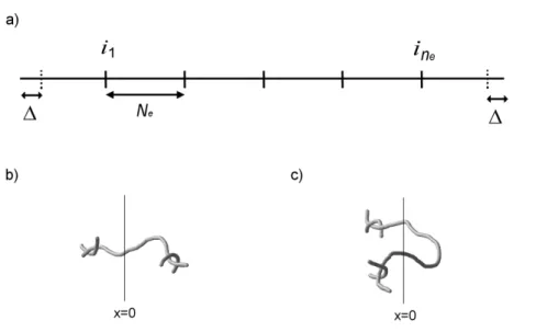
M therefore has on average n = M/Me segments and n − 1 entanglements. Due to the mean field approximation, in our derivation we will solve a single chain problem, and, to perform the calculations, it is necessary to assume that the exact number and position of the entanglements along the chain is known. What we can do is consider a real chain that has two dangling ends and forms an integer number of entanglements, given by ne= [n] − 1, where [x] denotes the integer part of x. Since the two ends of a chain are completely equivalent, it can be safely assumed that, on the average, entanglements are symmetrically distributed with respect to the chain center. Entanglements are therefore located at positions ik = kNe + ∆ along the chain, where ∆ = (N − Ne[n])/2 and k = 1, . . . , ne, as shown in Figure 3.1a.

Rigorously, the mean value of every physical quantity depending on the entangle-ment positions should be an appropriate average over all the possible configurations

(39)

3.1. Model of entanglements 31

Figure 3.1: (a) Position of the ne entanglements along the chain. Continuous bars represent entangled chains crossings while dashed ones are just an aid to the eye. Distances are expressed in number of monomer units. (b,c) Schematic representation of an effective (b) and a not effective (c) entanglement; the planar interface is defined by x=0.

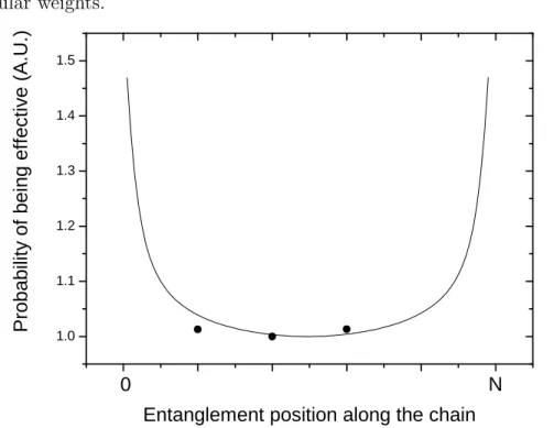
{ik}, but as a first approximation we treat the entanglement as fixed along the chain. This is done in the belief that, with an appropriate choice of the fixed configuration, a good approximation of the correct mean values can be obtained. To support this conclusion we will also show that Σeff changes little if the positions of all

entan-glements are translated along the chain. Unfortunately the configuration we chose has a number of entanglement ne that is different from their average number per chain n, so that in the numerical calculation we will need to normalize the com-puted Σeff. An alternative continuous approach that is able to directly consider the

correct average number of monomers per chain is presented in chapter 4. Another hypothesis assumed in our derivation is that the molecular weight of entanglement stays constant throughout the whole interface; this approximation is also discussed in chapter 4.

(40)

3.2 Calculation of the effective entanglement

den-sity for asymmetric interfaces

Chain coupling across the interface is described by the areal density of effectively entangled strands, Σeff. A strand is said to be effectively entangled if it connects two

subsequent entanglements placed on different sides of the interface, and is therefore able to transfer stress across the interface, as shown in Figures 3.1b and 3.1c.

In an asymmetric interface we assume that Σeff can be written as the sum of the

effective entanglements formed by the two polymers: Σeff = Σ(A)eff + Σ

(B)

eff . (3.2)

Calculations will be carried out for polymer A, and we will always refer to this species, unless otherwise stated. Derivations would obviously be the same for poly-mer B.

In order to solve the problem we introduce the Green function formalism. At thermodynamic equilibrium, the Green function G(r, r0_{; N), that we have already} introduced in chapter 2, represents the statistical weight of chains starting at r and ending at r0 _{in N steps, normalized with respect to the value it assumes in absence} of external fields. The Green function of a Gaussian chain in the presence of an external field Ue satisfies the following differential equation [5]

Ã ∂ ∂N − b2 6 ∂2 ∂r2 + 1 kBT Ue(r) ! G(r0_{, r; N) = δ(r − r}0_)δ(N), _(3.3) where the right hand side term is set so that it can satisfy the proper boundary conditions. We remark that the above formulation is completely equivalent to the Modified Diffusion Equation (2.11). For Ue = 0, the Green function gives the well known Gaussian distribution function

G0(r, r0; N) = Ã 2πNb2 3 !_−3/2 exp Ã −3(r − r 0₎2 2Nb2 ! . (3.4)

The mean values of any physical quantity depending on the position rn of the

(41)

3.2. Calculation of Σeff for asymmetric interfaces 33 hA(rn)i = R dr0drndrNG(r0, rn; n)G(rn, rN; N − n)A(rn) R dr0drNG(r0, rN; N) . (3.5)

If a quantity depends on the position of two monomers the corresponding expression for its mean value is

hA(rn, rm)i = R dr0drndrmdrNG(r0, rn; n)G(rn, rm; m − n)G(rm, rN; N − m)A(rn, rm) R dr0drNG(r0, rN; N) , (3.6) with m > n [5].

Since in the case of a plane interface the external potential depends only on one coordinate, that we identify as x, we can integrate on the other two and work in one dimension. The Green function G0 becomes

G0(x, x0; N) = βN √ π exp h −β2 N(x − x0) 2i _(3.7) with βN = q 3/2 N1/2_b. (3.8)

To compute Σeff it is necessary to count every strand that connects two

subse-quent entanglements placed on different sides of the interface, that we assume to be at x = 0. Working in a mean field approximation, it is sufficient to consider the single chain problem and then multiply the result by the number of chains. The operator that counts the total number of the coupling strands across the interface per unit area is

ˆ Σeff = ν A n_Xe−1 k=1 ·Z x<0dr Z x>0dr 0_δ(r ik− r)δ(rik+1− r 0₎ + Z x>0dr Z x<0dr 0_δ(r ik − r)δ(rik+1− r 0₎¸_, _(3.9)

(42)

where the sum over k counts entanglements along the chain, A is the system area and ν is the total number of chains. The density of effective entanglements per unit area can be expressed as the mean value of the above defined operator

Σeff = h ˆΣeffi. (3.10)

From eq.(3.6) we then obtain

Σeff = ν A 1 R R dr0drNG(r0, rN; N) × (3.11) n_Xe−1 k=1 ·Z x<0dr Z x>0dr 0 Z Z dr0drNG(r0, r; ik)G(r, r0; Ne)G(r0, rN; N − ik+1)+ Z x<0dr 0Z x>0dr Z Z dr0drNG(r0, r; ik)G(r, r0; Ne)G(r0, rN; N − ik+1) ¸ .

Integrating over y and z we obtain

Σeff = ν A 1 R q(x; N)dx × (3.12) n_Xe−1 k=1 ·Z ₀ −∞dx Z _∞ 0 dx 0_{q(x; i} k)G(x, x0; Ne)q(x0; N − ik+1)+ Z ₀ −∞dx 0Z ∞ 0 dxq(x; ik)G(x, x 0_{; N} e)q(x0; N − ik+1) ¸ .

where the notation

q(x; n) ≡

Z

G(x, x0_{; n)dx}0_, _(3.13) has been introduced.

Expression (3.12) can be simplified by noting that G(x, x0_{; m) = G(x}0_{, x; m) and} that, since we assumed entanglements symmetrically distributed with respect to the chain center, N − ik+1 = ine−k. Using these relationships it is possible to write

Z ₀ −∞dx 0Z ∞ 0 dx n_Xe−1 k=1 q(x; ik)G(x, x0; Ne)q(x0; N − ik+1) = (3.14)

(43)

3.2. Calculation of Σeff for asymmetric interfaces 35 = Z ₀ −∞dx 0Z ∞ 0 dx n_Xe−1 k=1 q(x0; ik)G(x0, x; Ne)q(x; N − ik+1), and finally Σeff = ν A 2 R Lq(x; N)dx × (3.15) n_Xe−1 k=1 ·Z ₀ −∞dx Z _∞ 0 dx 0_{q(x; i} k)G(x, x0; Ne)q(x0; N − ik+1) ¸ ,

where L is the dimension of the system in the x direction. The total number of chains can be written as

ν = 1 N Z V ρ(r)dr = ρbA N Z Lφ(x)dx, (3.16) where ρ(r) is the total density of monomers, φ(x) = ρ(x)_ρ

b is the polymer volume

fraction, ρb is the bulk monomer density and V is the system volume. Substituting equation (3.16) into equation (3.15) one derives

Σeff = 2ρb N R Lφ(x)dx R Lq(x; N)dx × (3.17) n_Xe−1 k=1 ·Z ₀ −∞dx Z _∞ 0 dx 0_{q(x; i} k)G(x, x0; Ne)q(x0; N − ik+1) ¸ .

Finally observe that in the homogeneous phases φ(±∞) = q(±∞; N), as follows from equation (2.57), so that for a system where L is much greater than the interface width we have lim L→∞ R Lφ(x)dx R Lq(x; N)dx = 1. (3.18)

The final expression for Σeff is therefore

Σeff = 2ρb N n_Xe−1 k=1 ·Z ₀ −∞dx Z _∞ 0 dx 0_{q(x; i} k)G(x, x0; Ne)q(x0; N − ik+1) ¸ . (3.19)

(44)

This equation gives the density of effective entanglements formed by one polymer across the interface. The total density is the sum of the contributions by both species. Expression (3.19) is the main result of this section.

In the case of an A/A interface, Ue = 0, φ(x) ≡ 1, G(x, x0; Ne) = G0(x, x0; Ne) and q(x; i) ≡ 1 ∀i, so that from equation (3.19) it holds

Σeff = 2ρb N (ne− 1) ·Z ₀ −∞dx 1 2[1 + Erf(βNex)] ¸ . (3.20)

If the total number of entanglements is the real number ne = n − 1, then the final result in the symmetric case reads

Σeff = ρb(n − 2) NβNe √ π = ρeLe q 3π/2 µ 1 −2Me M ¶ , (3.21)

where we used ρe = ρb/Ne and Le = b

√

Ne. Equation (3.21) is exactly the same result that was obtained by Mikos and Peppas [2]. We also note that, except for chain end effects, the result is very similar to the one obtained with the simple Lake and Thomas approach, since q3π/2 ≈ 2.17.

3.2.1 Long chains approximation

Expression (3.19) is quite lengthy to evaluate and it may obscure the essential fea-tures of our model. Nevertheless it is possible to derive an excellent approximation in the case of long chains.

In a ν chains system, the density of the nth monomers along the chains is given by

ρn(x) = νhδ(x − xn)i =

ρb

Nq(x; n)q(x; N − n). (3.22)

In general the density profiles ρn(x) are not uniform and are functions of n, that indicates the position along the chain, through q(x; n). For infinite chains, we can neglect the chain end effects and we can imagine that all the monomers are infinitely distant from the chain ends, so that q(x; n) approaches a function q(x; ∞)