DOI:10.1051/0004-6361/201527101 c ESO 2016
Astronomy
&
Astrophysics
Planck 2015 results
Special feature
Planck 2015 results
I. Overview of products and scientific results
Planck Collaboration: R. Adam105, P. A. R. Ade126, N. Aghanim84, Y. Akrami89, 148, M. I. R. Alves143, 14, 84, F. Argüeso28, M. Arnaud103,
F. Arroja94, 109, M. Ashdown98, 9, J. Aumont84, C. Baccigalupi123, M. Ballardini46, 70, 72, A. J. Banday143, 14, R. B. Barreiro92, J. G. Bartlett1, 95,
N. Bartolo45, 94, S. Basak123, P. Battaglia48, 50, E. Battaner146, 147, R. Battye96, K. Benabed85, 140, A. Benoît82, A. Benoit-Lévy35, 85, 140,
J.-P. Bernard143, 14, M. Bersanelli49, 71, B. Bertincourt84, P. Bielewicz116, 14, 123, I. Bikmaev30, 4, J. J. Bock95, 16, H. Böhringer111, A. Bonaldi96,
L. Bonavera26, J. R. Bond13, J. Borrill19, 131, F. R. Bouchet85, 129, F. Boulanger84, M. Bucher1, R. Burenin130, 113, C. Burigana70, 47, 72, R. C. Butler70,
E. Calabrese135, J.-F. Cardoso104, 1, 85, P. Carvalho88, 98, B. Casaponsa92, G. Castex1, A. Catalano105, 101, A. Challinor88, 98, 17, A. Chamballu103, 21, 84,
R.-R. Chary81, H. C. Chiang39, 10, J. Chluba34, 98, G. Chon111, P. R. Christensen117, 53, S. Church133, M. Clemens67, D. L. Clements80,
S. Colombi85, 140, L. P. L. Colombo33, 95, C. Combet105, B. Comis105, D. Contreras32, F. Couchot100, A. Coulais101, B. P. Crill95, 16, M. Cruz27,
A. Curto92, 9, 98, F. Cuttaia70, L. Danese123, R. D. Davies96, R. J. Davis96, P. de Bernardis48, A. de Rosa70, G. de Zotti67, 123, J. Delabrouille1,
J.-M. Delouis85, 140, F.-X. Désert77, E. Di Valentino85, 129, C. Dickinson96, J. M. Diego92, K. Dolag145, 110, H. Dole84, 83, S. Donzelli71, O. Doré95, 16,
M. Douspis84, A. Ducout85, 80, J. Dunkley135, X. Dupac57, G. Efstathiou98, 88, P. R. M. Eisenhardt95, F. Elsner35, 85, 140, T. A. Enßlin110,
H. K. Eriksen89, E. Falgarone101, Y. Fantaye52, 5, M. Farhang13, 122, S. Feeney80, J. Fergusson17, R. Fernandez-Cobos92, F. Feroz9, F. Finelli70, 72,
E. Florido146, O. Forni143, 14, M. Frailis69, A. A. Fraisse39, C. Franceschet49, E. Franceschi70, A. Frejsel117, A. Frolov128, S. Galeotta69, S. Galli97,
K. Ganga1, C. Gauthier1, 109, R. T. Génova-Santos91, 25, M. Gerbino138, 119, 48, T. Ghosh84, M. Giard143, 14, Y. Giraud-Héraud1, E. Giusarma48,
E. Gjerløw89, J. González-Nuevo26, 92, K. M. Górski95, 150, K. J. B. Grainge9, 98, S. Gratton98, 88, A. Gregorio50, 69, 76, A. Gruppuso70, 72,
J. E. Gudmundsson138, 119, 39, J. Hamann139, 136, W. Handley98, 9, F. K. Hansen89, D. Hanson112, 95, 13, D. L. Harrison88, 98, A. Heavens80, G. Helou16,
S. Henrot-Versillé100, C. Hernández-Monteagudo18, 110, D. Herranz92, S. R. Hildebrandt95, 16, E. Hivon85, 140, M. Hobson9, W. A. Holmes95,
A. Hornstrup22, W. Hovest110, Z. Huang13, K. M. Huffenberger37, G. Hurier84, S. Ili´c143, 14, 8, A. H. Jaffe80, T. R. Jaffe143, 14, T. Jin9, W. C. Jones39,
M. Juvela38, A. Karakci1, E. Keihänen38, R. Keskitalo19, I. Khamitov137, 30, K. Kiiveri38, 64, J. Kim110, T. S. Kisner107, R. Kneissl55, 11,
J. Knoche110, L. Knox42, N. Krachmalnicoff49, M. Kunz23, 84, 5, H. Kurki-Suonio38, 64, F. Lacasa84, 65, G. Lagache7, 84, A. Lähteenmäki2, 64,
J.-M. Lamarre101, M. Langer84, A. Lasenby9, 98, M. Lattanzi47, 73, C. R. Lawrence95,?, M. Le Jeune1, J. P. Leahy96, E. Lellouch102, R. Leonardi12,
J. León-Tavares90, 59, 3, J. Lesgourgues86, 139, F. Levrier101, A. Lewis36, M. Liguori45, 94, P. B. Lilje89, M. Lilley85, 129, M. Linden-Vørnle22,
V. Lindholm38, 64, H. Liu117, 53, M. López-Caniego57, P. M. Lubin43, Y.-Z. Ma96, 125, J. F. Macías-Pérez105, G. Maggio69, D. Maino49, 71,
D. S. Y. Mak88, 98, N. Mandolesi70, 47, A. Mangilli84, 100, A. Marchini74, A. Marcos-Caballero92, D. Marinucci52, M. Maris69, D. J. Marshall103,
P. G. Martin13, M. Martinelli148, E. Martínez-González92, S. Masi48, S. Matarrese45, 94, 61, P. Mazzotta51, J. D. McEwen114, P. McGehee81,
S. Mei60, 142, 16, P. R. Meinhold43, A. Melchiorri48, 74, J.-B. Melin21, L. Mendes57, A. Mennella49, 71, M. Migliaccio88, 98, K. Mikkelsen89,
M. Millea42, S. Mitra79, 95, M.-A. Miville-Deschênes84, 13, D. Molinari47, 70, 73, A. Moneti85, L. Montier143, 14, R. Moreno102, G. Morgante70,
D. Mortlock80, A. Moss127, S. Mottet85, 129, M. Münchmeyer85, D. Munshi126, J. A. Murphy115, A. Narimani32, P. Naselsky118, 54, A. Nastasi84,
F. Nati39, P. Natoli47, 6, 73, M. Negrello67, C. B. Netterfield29, H. U. Nørgaard-Nielsen22, F. Noviello96, D. Novikov108, I. Novikov117, 108,
M. Olamaie9, N. Oppermann13, E. Orlando149, C. A. Oxborrow22, F. Paci123, L. Pagano48, 74, F. Pajot84, R. Paladini81, S. Pandolfi24,
D. Paoletti70, 72, B. Partridge63, F. Pasian69, G. Patanchon1, T. J. Pearson16, 81, M. Peel96, H. V. Peiris35, V.-M. Pelkonen81, O. Perdereau100,
L. Perotto105, Y. C. Perrott9, F. Perrotta123, V. Pettorino62, F. Piacentini48, M. Piat1, E. Pierpaoli33, D. Pietrobon95, S. Plaszczynski100,
D. Pogosyan40, E. Pointecouteau143, 14, G. Polenta6, 68, L. Popa87, G. W. Pratt103, G. Prézeau16, 95, S. Prunet85, 140, J.-L. Puget84, J. P. Rachen31, 110,
B. Racine89, W. T. Reach144, R. Rebolo91, 20, 25, M. Reinecke110, M. Remazeilles96, 84, 1, C. Renault105, A. Renzi52, 75, I. Ristorcelli143, 14,
G. Rocha95, 16, M. Roman1, E. Romelli50, 69, C. Rosset1, M. Rossetti49, 71, A. Rotti79, G. Roudier1, 101, 95, B. Rouillé d’Orfeuil100,
M. Rowan-Robinson80, J. A. Rubiño-Martín91, 25, B. Ruiz-Granados146, C. Rumsey9, B. Rusholme81, N. Said48, V. Salvatelli48, 8, L. Salvati48,
M. Sandri70, H. S. Sanghera88, 98, D. Santos105, R. D. E. Saunders9, A. Sauvé143, 14, M. Savelainen38, 64, G. Savini120, B. M. Schaefer141,
M. P. Schammel9, 93, D. Scott32, M. D. Seiffert95, 16, P. Serra84, E. P. S. Shellard17, T. W. Shimwell9, 134, M. Shiraishi45, 94, K. Smith121,
T. Souradeep79, L. D. Spencer126, M. Spinelli100, S. A. Stanford42, D. Stern95, V. Stolyarov9, 132, 99, R. Stompor1, A. W. Strong111, R. Sudiwala126,
R. Sunyaev110, 130, P. Sutter85, D. Sutton88, 98, A.-S. Suur-Uski38, 64, J.-F. Sygnet85, J. A. Tauber58, D. Tavagnacco69, 50, L. Terenzi124, 70, D. Texier56,
L. Toffolatti26, 92, 70, M. Tomasi49, 71, M. Tornikoski3, D. Tramonte91, 25, M. Tristram100, A. Troja49, T. Trombetti70, 47, M. Tucci23, J. Tuovinen15,
M. Türler78, G. Umana66, L. Valenziano70, J. Valiviita38, 64, F. Van Tent106, T. Vassallo69, L. Vibert84, M. Vidal96, M. Viel69, 76, P. Vielva92,
F. Villa70, L. A. Wade95, B. Walter63, B. D. Wandelt85, 140, 44, R. Watson96, I. K. Wehus95, 89, N. Welikala135, J. Weller145, M. White41,
S. D. M. White110, A. Wilkinson96, D. Yvon21, A. Zacchei69, J. P. Zibin32, and A. Zonca43
(Affiliations can be found after the references) Received 1 August 2015/ Accepted 18 January 2016
ABSTRACT
The European Space Agency’s Planck satellite, which is dedicated to studying the early Universe and its subsequent evolution, was launched on 14 May 2009. It scanned the microwave and submillimetre sky continuously between 12 August 2009 and 23 October 2013. In February 2015, ESA and the Planck Collaboration released the second set of cosmology products based on data from the entire Planck mission, including both temperature and polarization, along with a set of scientific and technical papers and a web-based explanatory supplement. This paper gives an overview of the main characteristics of the data and the data products in the release, as well as the associated cosmological and astrophysical science results and papers. The data products include maps of the cosmic microwave background (CMB), the thermal Sunyaev-Zeldovich effect, diffuse foregrounds in temperature and polarization, catalogues of compact Galactic and extragalactic sources (including separate catalogues of
Sunyaev-Zeldovich clusters and Galactic cold clumps), and extensive simulations of signals and noise used in assessing uncertainties and the performance of the analysis methods. The likelihood code used to assess cosmological models against the Planck data is described, along with a CMB lensing likelihood. Scientific results include cosmological parameters derived from CMB power spectra, gravitational lensing, and cluster counts, as well as constraints on inflation, non-Gaussianity, primordial magnetic fields, dark energy, and modified gravity, and new results on low-frequency Galactic foregrounds.
Key wordscosmology: observations – cosmic background radiation – surveys – space vehicles: instruments – instrumentation: detectors
1. Introduction
The Planck satellite1(Tauber et al. 2010;Planck Collaboration I 2011), launched on 14 May 2009, observed the sky continu-ously from 12 August 2009 to 23 October 2013. Planck’s sci-entific payload contained an array of 74 detectors in nine bands covering frequencies between 25 and 1000 GHz, which scanned the sky with angular resolution between 330 and 50. The
de-tectors of the Low Frequency Instrument (LFI;Bersanelli et al. 2010; Mennella et al. 2011) were pseudo-correlation radiome-ters, covering bands centred at 30, 44, and 70 GHz. The de-tectors of the High Frequency Instrument (HFI; Lamarre et al. 2010;Planck HFI Core Team 2011) were bolometers, covering bands centred at 100, 143, 217, 353, 545, and 857 GHz. Planck imaged the whole sky twice in one year, with a combination of sensitivity, angular resolution, and frequency coverage never be-fore achieved. Planck, its payload, and its performance as pre-dicted at the time of launch are described in 13 papers included in a special issue of Astronomy & Astrophysics (Volume 520).
The main objective of Planck, defined in 1995, was to measure the spatial anisotropies in the temperature of the cos-mic cos-microwave background (CMB), with an accuracy set by fundamental astrophysical limits, thereby extracting essentially all the cosmological information embedded in the temperature anisotropies of the CMB. Planck was not initially designed to measure to high accuracy the CMB polarization anisotropies, which encode not only a wealth of cosmological information, but also provide a unique probe of the history of the Universe dur-ing the time when the first stars and galaxies formed. However, during Planck’s development it was significantly enhanced in this respect, and its polarization measurement capabilities have exceeded all original expectations. Planck was also designed to produce a wealth of information on the properties of extra-galactic sources, including clusters of galaxies via the Sunyaev-Zeldovich (SZ) effect, and the dust and gas in the Milky Way. The scientific objectives of Planck were described in detail in Planck Collaboration(2005). With the results presented here and in a series of accompanying papers, Planck has already achieved all of its planned science goals.
An overview of the scientific operations of the Planck mis-sion was given inPlanck Collaboration I(2014). Further opera-tional details extending to the end of the mission are presented in the 2015 Explanatory Supplement (Planck Collaboration 2015). The first set of scientific data, the Early Release Compact Source Catalogue (ERCSC; Planck Collaboration VII 2011), was re-leased in January 2011. At the same time, a set of 26 papers related to astrophysical foregrounds were published in a special issue of Astronomy and Astrophysics (Vol. 536, 2011). Since then, 40 “Intermediate” (i.e., between the major data releases) papers have been submitted to A&A containing further astro-physical investigations by the Collaboration. The second set of 1 Planck(http://www.esa.int/Planck) is a project of the
Euro-pean Space Agency (ESA) with instruments provided by two scientific consortia funded by ESA member states and led by Principal Investi-gators from France and Italy, telescope reflectors provided through a collaboration between ESA and a scientific consortium led and funded by Denmark, and additional contributions from NASA (USA).
scientific data (sometimes referred to as Planck Release 1 or “PR1”, because it was the first release of cosmologically use-ful data) consisting mainly of temperature maps of the whole sky, was released in March of 2013. These data and associated scientific results are described in a set of 32 papers in another special issue of A&A (Vol. 571, 2014). This paper presents an overview of the third set of scientific data (and second set of cosmological data, hence “PR2”) and scientific results to be re-leased by Planck, based on the data acquired during the complete Planckmission from 12 August 2009 to 23 October 2013, and hereafter referred to as the “2015 products”.
2. Data products in the 2015 release
The 2015 distribution of released products, freely accessible via the Planck Legacy Archive interface (PLA)2, is based on all the data acquired by Planck during routine operations, starting on 12 August 2009 and ending on 23 October 2014. The distribution contains the following items.
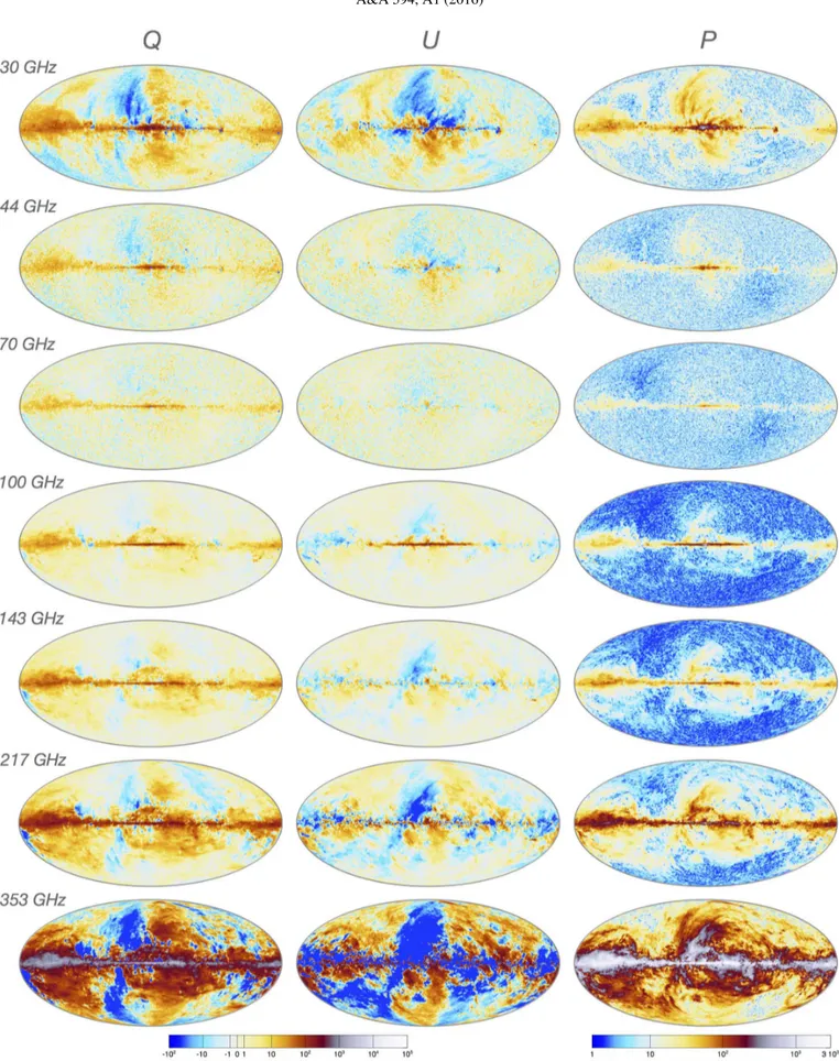
– Cleaned and calibrated data timelines for each detector. – Maps of the sky at nine frequencies (Sect. 7) in
temper-ature, and at seven frequencies (30–353 GHz) in polariza-tion. Additional products serve to quantify the characteris-tics of the maps to a level adequate for the science results being presented, such as noise maps, masks, and instrument characteristics.
– High-resolution maps of the CMB sky in temperature from four different component-separation approaches, and accom-panying characterization products (Sect.8.1).
– High-pass-filtered maps of the CMB sky in polarization from four different component-separation approaches, and accom-panying characterization products (Sect.8.1). The rationale for providing these maps is explained in Sect.2.2.
– A low-resolution CMB temperature map (Sect.8.1) used in the low-` likelihood code, with an associated set of fore-ground temperature maps produced as part of the process of separating the low-resolution CMB from foregrounds, with accompanying characterization products.
– Maps of thermal dust and residual cosmic infrared back-ground (CIB) fluctuations, as well as carbon monoxide (CO), synchrotron, free-free, and spinning dust temperature emis-sion, plus maps of dust temperature and opacity (Sect.9). – Maps of synchrotron and dust polarized emission.
– A map of the estimated CMB lensing potential over 70% of the sky.
– A map of the SZ effect Compton parameter.
– Monte Carlo chains used in determining cosmological pa-rameters from the Planck data.
– The Second Planck Catalogue of Compact Sources (PCCS2; Sect.9.1), comprising lists of compact sources over the entire sky at the nine Planck frequencies. The PCCS2 includes po-larization information, and supersedes the previous Early Re-lease Compact Source Catalogue (Planck Collaboration XIV 2011) and the PCCS1 (Planck Collaboration XXVIII 2014).
– The Second Planck Catalogue of Sunyaev-Zeldovich Sources (PSZ2; Sect.9.2), comprising a list of sources de-tected by their SZ distortion of the CMB spectrum. The PSZ2 supersedes the previous Early Sunyaev-Zeldovich Cat-alogue (Planck Collaboration XXIX 2014) and the PSZ1 (Planck Collaboration XXIX 2014).
– The Planck Catalogue of Galactic Cold Clumps (PGCC; Planck Collaboration XXVIII 2016), providing a list of Galactic cold sources over the whole sky (see Sect.9.3). The PGCC supersedes the previous Early Cold Core Catalogue (ECC), part of the Early Release Compact Source Catalogue (ERCSC;Planck Collaboration VII 2011).
– A full set of simulations, including Monte Carlo realizations. – A likelihood code and data package used for testing cosmo-logical models against the Planck data, including both the CMB (Sect.8.4.1) and CMB lensing (Sect.8.4.2).
The first 2015 products were released in February 2015, polar-ized maps and time-ordered data were released in July 2015, and simulations were released in September 2015 (see Sect. 4). In parallel, the Planck Collaboration is developing the next genera-tion of data products, which will be delivered in 2016.
2.1. Polarization convention
The Planck Stokes parameter maps and data follow the “COSMO”3convention for polarization angles, rather than the “IAU” (Heeschen & Howard 1974;Hamaker & Bregman 1996) convention. The net effect of using the COSMO convention is a sign inversion on Stokes U with respect to the IAU convention (position angle increases clockwise in the IAU convention, an-ticlockwise in the IAU convention). On the other hand, when polarization angles are discussed in Planck Collaboration pa-pers, they are given in the IAU convention (e.g., in the Planck Catalogue of Compact Sources, Planck Collaboration XXVIII 2014; the Second Planck Catalogue of Compact Sources, Planck Collaboration XXVI 2016; and papers on foregrounds), with position angle zero being the direction of the north Galactic pole. All Planck FITS files containing polarization data include a keyword (POLCCONV) that specifies the convention used, and the text and figures of papers also specify the convention. Users should be aware, however, of this potential source of confusion. 2.2. The state of polarization in the Planck 2015 data
LFI – The 2015 Planck release includes polarization data at 30, 44, and 70 GHz. The 70 GHz polarization data are used for the 2015 Planck likelihood at ` < 30. The 70 GHz map is cleaned with the 30 and 353 GHz channels for synchrotron and dust emission, respectively (Planck Collaboration XIII 2016).
Control of systematic effects in polarization is a challenging task, especially at large angular scales. We analyse systematic ef-fects in the 2015 LFI polarization data (Planck Collaboration III 2016) following two complementary paths. First, we use the re-dundancy in the Planck scanning strategy to produce difference maps that, in principle, contain the same sky signal (“null tests”). Any residuals in these maps blindly probe all non-common-mode systematics present in the data. Second, we use our knowl-edge of the instrument to build physical models of all relevant systematic effects. We then simulate timelines and project them into sky maps following the LFI map-making process. We quan-tify the results in terms of power spectra, and compare them to the FFP8 LFI noise model.
3 See http://healpix.sourceforge.net/html/intronode6.
htm.
Our analysis shows no evidence of systematic errors signif-icantly affecting the 2015 LFI polarization results. On the other hand, our model indicates that at low multipoles the dominant LFI systematics (gain errors and ADC nonlinearity) are only marginally dominated by noise and the expected signal. There-fore, further independent tests are being carried out and will be discussed in a forthcoming paper, as well as in the final 2016 Planckrelease. These include polarization cross-spectra between the LFI 70 GHz and the HFI 100 and 143 GHz maps (that are not part of this 2015 release; see below). Because systematic effects between the two Planck instruments are expected to be largely uncorrelated, such a cross-instrument approach may prove par-ticularly effective.
HFI – The February 2015 data release included polarization data at 30, 44, 70, and 353 GHz. The release of the remaining three polarized HFI channels – 100, 143, and 217 GHz – was de-layed because of residual systematic errors in the polarization data, particularly but not exclusively at ` < 10. The sources of these systematic errors were identified, but insufficiently char-acterized to support reliable scientific analyses of, for example, the optical depth to ionization τ and the isotropy and statistics of the polarization fluctuations. Due to an internal mixup, how-ever, the unfiltered polarized sky maps ended up in the PLA in-stead of the high-pass-filtered ones. This was discovered in July 2015, and the high-pass-filtered maps at 100, 143, and 217 GHz were added to the PLA. The unfiltered maps have been left in place to avoid confusion, but warnings about their unsuitabil-ity for science have been added. Since February our knowledge of the causes of residual systematic errors and our characteriza-tion of the polarizacharacteriza-tion maps have improved. Problems that users might encounter in the released 100–353 GHz maps include the following:
– Null tests on data splits indicate inconsistency of polariza-tion measurements on large angular scales at a level much larger than our instrument noise model (see Fig. 10 of Planck Collaboration VIII 2016). The reasons for this are nu-merous and will be described in detail in a future paper. – While analogue-to-digital converter (ADC) nonlinearity is
corrected much better than in previous releases, some resid-ual effects remain, particularly in the distortion of the dipole that leaks dipole power to higher spatial frequencies. – Mismatches in bandpasses result in leakage of dust
tempera-ture to polarization, particularly on large angular scales. – While the measured beam models are improved, main beam
mismatches cause temperature-to-polarization leakage in the maps (see Fig. 17 ofPlanck Collaboration VII 2016). In pro-ducing the results given in the Planck 2015 release, we cor-rect for this at the spectrum level (Planck Collaboration XI 2016), but the maps themselves contain this effect.
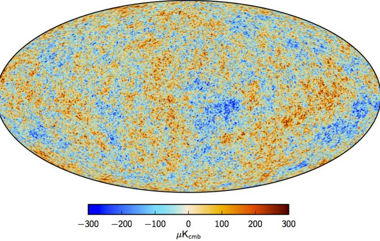
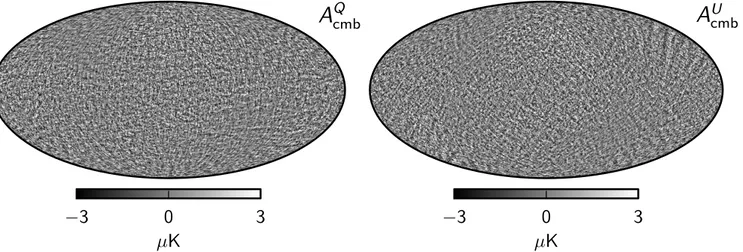
The component-separation work described in Sect. 9, Planck Collaboration IX (2016), and Planck Collaboration X (2016) was performed on all available data, and produced un-precedented full-sky polarization maps of foreground emission (Figs.22and24), as well as maps of polarized CMB emission. The polarized CMB maps, derived using four independent component-separation methods, were the basis for quantitative statements about the level of residual polarization systematics and the conclusion that reliable science results could not be obtained from them on the largest angular scales.
Recent improvements in mapmaking methodology that re-duce the level of residual systematic errors in the maps, espe-cially at low multipoles, will be described in a future paper. A
more fundamental ongoing effort aimed at correcting system-atic polarization effects in the time-ordered data will produce the final legacy Planck data, to be released in 2016.
3. Papers accompanying the 2015 release
The characteristics, processing, and analysis of the Planck data, as well as a number of scientific results, are described in a series of papers released with the data. The titles of the papers begin with “Planck 2015 results”, followed by the specific titles below. I. Overview of products and scientific results (this paper) II. Low Frequency Instrument data processing
III. LFI systematic uncertainties IV. LFI beams and window functions V. LFI calibration
VI. LFI mapmaking
VII. High Frequency Instrument data processing: Time-ordered information and beam processing
VIII. High Frequency Instrument data processing: Calibration and maps
IX. Diffuse component separation: CMB maps X. Diffuse component separation: Foreground maps XI. CMB power spectra, likelihoods, and robustness of
parameters XII. Simulations
XIII. Cosmological parameters XIV. Dark energy and modified gravity XV. Gravitational lensing
XVI. Isotropy and statistics of the CMB
XVII. Constraints on primordial non-Gaussianity
XVIII. Background geometry and topology of the Universe XIX. Constraints on primordial magnetic fields
XX. Constraints on inflation
XXI. The integrated Sachs-Wolfe effect
XXII. A map of the thermal Sunyaev-Zeldovich effect
XXIII. The thermal Sunyaev-Zeldovich effect–cosmic infrared background correlation
XXIV. Cosmology from Sunyaev-Zeldovich cluster counts XXV. Diffuse low-frequency Galactic foregrounds XXVI. The Second Planck Catalogue of Compact Sources XXVII. The Second Planck Catalogue of Sunyaev-Zeldovich
Sources
XXVIII. The Planck Catalogue of Galactic Cold Clumps This paper contains an overview of the main aspects of the Planck project that have contributed to the 2015 release, and points to the papers that contain full descriptions. It proceeds as follows. Section 4 describes the simulations that have been generated to support the analysis of Planck data. Section5 de-scribes the basic processing steps leading to the generation of the Planck timelines. Section 6 describes the timelines them-selves. Section7describes the generation of the nine Planck fre-quency maps and their characteristics. Section 8 describes the Planck 2015 products related to the cosmic microwave back-ground, namely the CMB maps, the lensing products, and the likelihood code. Section9describes the Planck 2015 astrophysi-cal products, including catalogues of compact sources and maps of diffuse foreground emission. Section10describes the main
cosmological science results based on the 2015 CMB products. Section11describes some of the astrophysical results based on the 2015 data. Section12concludes with a summary and a look towards future Planck products.
4. Simulations
We simulated time-ordered information (TOI) for the full fo-cal plane (FFP) for the nominal mission. The first five FFP realizations were less comprehensive and were primarily used for validation and verification of the Planck analysis codes and for cross-validation of the data processing centre (DPC) and FFP simulation pipelines. The first Planck cosmology results (Planck Collaboration I 2014) were supported primarily by the sixth FFP simulation set, FFP6. The current results were sup-ported by the eighth FFP simulation set, FFP8, which is de-scribed in detail inPlanck Collaboration XII(2016).
Each FFP simulation comprises a single “fiducial” realiza-tion (CMB, astrophysical foregrounds, and noise), together with separate Monte Carlo (MC) realizations of the CMB and noise. The CMB component contains the effect of our motion with respect to the CMB rest frame. This induces an additive dipo-lar aberration, a frequency-dependent dipole modulation, and a frequency-dependent quadrupole in the CMB data. Of these ef-fects, the additive dipole and frequency-independent component of the quadrupole are removed (see Planck Collaboration XII 2016for details), while the residual quadrupole and modulation effects are left in the simulations and are also left in the LFI and HFI data. The residual aberration contribution to the Doppler boosting was planned to be left in the simulations; however, due to a bug in the code generating the CMB realizations, it was in-advertently omitted. New, corrected, realizations are being gen-erated, and will be added to the public data release when they become available. This effect remains in the LFI and HFI data.
To mimic the Planck data as closely as possible, the sim-ulations use the actual pointing, data flags, detector bandpasses, beams, and noise properties of the nominal mission. For the fidu-cial realization, maps were made of the total observation (CMB, foregrounds, and noise) at each frequency for the nominal mis-sion period, using the Planck Sky Model (Delabrouille et al. 2013). In addition, maps were made of each component sep-arately, of subsets of detectors at each frequency, and of half-ring and single Survey subsets of the data. The noise and CMB Monte Carlo realization-sets also included both all and subsets of detectors (so-called “DetSets”) at each frequency, and full and half-ring data sets for each detector combination.
To check that the 2015 results are not sensitive to the exact cosmological parameters used in FFP8, we subsequently gener-ated FFP8.1, exactly matching the PR2 (2015) cosmology.
All of the FFP8 and FFP8.1 simulations are available to be used at NERSC4; in addition, a limited subset of the simulations is available for download from the PLA.
5. Data processing
5.1. Timeline processing 5.1.1. LFI
The main changes in LFI data processing compared to the earlier release (Planck Collaboration II 2014) are in how we account for beam information in the pipeline, and in calibration. Processing starts at Level 1, which retrieves necessary information from data packets and auxiliary data received from the Mission Operation
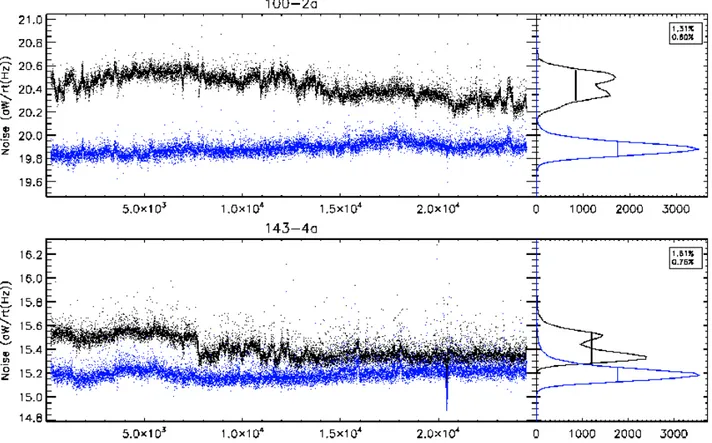
Fig. 1. Left panels: noise for two bolometers as a function of ring number. Black dots are from the 2013 data release; blue dots are from the 2015 release. The change in the absolute noise level is due to a change in the time-response deconvolution between the two data releases. Right panels: histograms of the noise. The numbers in the boxes give the width of the histogram at half maximum as a percentage of the mean noise level. For most bolometers, the FWHM in the 2015 release is less than 1% (Planck Collaboration VIII 2016).
Centre, and transforms the scientific packets and housekeeping data into a form manageable by Level 2. Level 2 uses scientific and housekeeping information to:
– build the LFI reduced instrument model (RIMO), which con-tains the main characteristics of the instrument;
– remove ADC nonlinearities and 1 Hz spikes diode by diode; – compute and apply the gain modulation factor to minimize
1/ f noise;
– combine signals from the diodes with associated weights; – compute the appropriate detector pointing for each sample,
based on auxiliary data and beam information, corrected by a model (PTCOR) built using Solar distance and radiometer electronics box assembly (REBA) temperature information; – calibrate the scientific timelines in physical units (KCMB),
fit-ting the total CMB dipole convolved with the 4π beam rep-resentation, without taking into account the signature due to Galactic stray light;
– remove the Solar and orbital dipoles (convolved with the 4π beam) and the Galactic emission (convolved with the beam sidelobes) from the scientific calibrated timeline; and – combine the calibrated time-ordered information (TOI) into
aggregate products, such as maps at each frequency. Level 3 collects Level 2 outputs from both LFI and HFI (Planck Collaboration VI 2016; Planck Collaboration VIII 2016) and derives various products, such as component-separated maps of astrophysical foregrounds, catalogues of dif-ferent classes of source, and the likelihood of cosmological and astrophysical models given in the maps.
5.1.2. HFI
The most important change in HFI data processing compared to the 2013 release (Planck Collaboration VI 2014) is in the very first step of the pipeline, namely correction of nonlin-earity in the 16-bit analogue-to-digital converters (ADCs) that are the last component in the bolometer readout electronics (Planck Collaboration 2015). The subtle effects of the ADC non-linearities that mimic gain variations were neither detected in ground tests nor anticipated before flight, but proved to be the source of the most difficult systematic errors to deal with in the flight data. A method that reduces the effects of ADC nonlinear-ity by more than an order of magnitude for most channels has been implemented. Improvements can be assessed by compar-ing the noise stationarity in the 2013 and the 2015 data (Fig.1). There is a significant decrease in the width of the noise distribu-tions when the ADC correction is included.
Several other changes were also made in processing for the 2015 release. For strong signals, the threshold for cos-mic ray removal (“deglitching”) is auto-adjusted to cope with signal variations near bright sources caused by small point-ing drifts durpoint-ing a rpoint-ing. Thus, more glitches are left in the data in the vicinity of bright sources such as the Galactic cen-tre than are left elsewhere. To mitigate this effect, the TOI at the planet locations are flagged and interpolated prior to fur-ther processing. For the 2015 release, this is done for Jupiter at all HFI frequency bands, for Saturn at ν ≥ 217 GHz, and for Mars at ν ≥ 353 GHz. For beam determination and cali-bration (see Sect. 5.2.2 of Planck Collaboration VII 2016 and Planck Collaboration VIII 2016), however, the full TOI at all planet crossings are needed at all frequencies. To recover these
0 10 20 30 40 50
Fraction of flagged data [%]
00_100_1a 01_100_1b 20_100_2a 21_100_2b 40_100_3a 41_100_3b 80_100_4a 81_100_4b 02_143_1a 03_143_1b 30_143_2a 31_143_2b 50_143_3a 51_143_3b 82_143_4a 83_143_4b 10_143_5 42_143_6 60_143_7 11_217_5a 12_217_5b 43_217_6a 44_217_6b 61_217_7a 62_217_7b 71_217_8a 72_217_8b 04_217_1 22_217_2 52_217_3 84_217_4 23_353_3a 24_353_3b 32_353_4a 33_353_4b 53_353_5a 54_353_5b 63_353_6a 64_353_6b 05_353_1 13_353_2 45_353_7 85_353_8 14_545_1 34_545_2 73_545_4 25_857_1 35_857_2 65_857_3 74_857_4
sample+ring flag sample flag Individual glitch flag
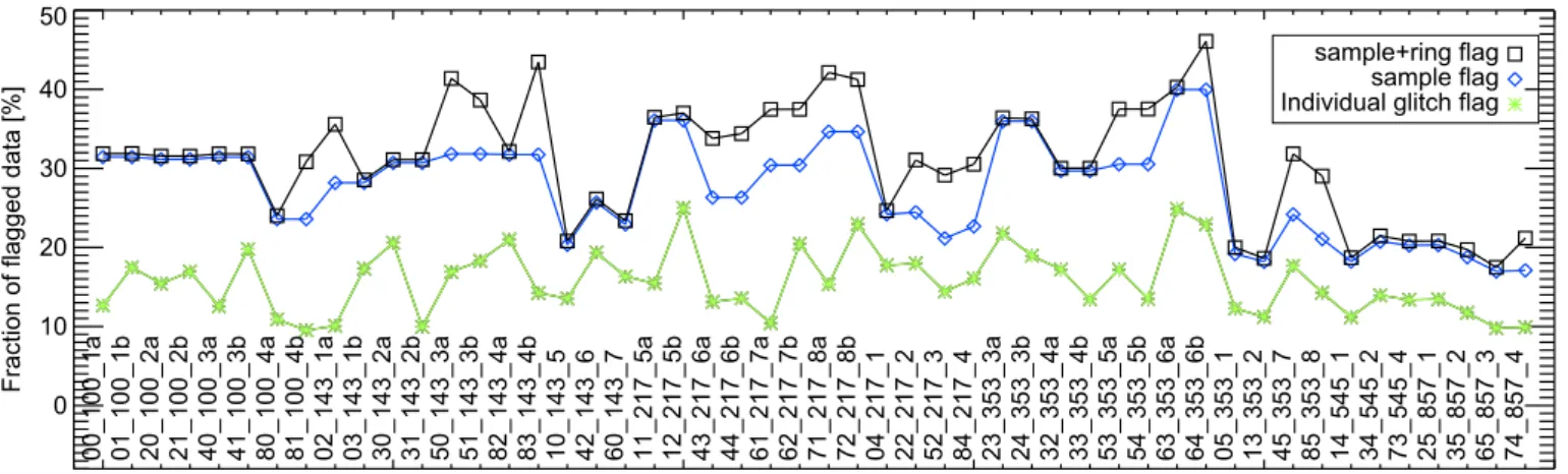
Fig. 2.Fraction of discarded data per bolometer due to all causes (black squares), sample flagging alone (blue diamonds) and glitches alone (green
diamonds). Bolometers (143_8 and 545_3) are not shown, since they are not used in the data processing (seePlanck Collaboration VI 2014).
data in 2015, a specialized, iterative, 3-level deglitcher is run in parallel on TOI in the vicinity of strong sources.
As noted inPlanck Collaboration I (2014), Planck scans a given ring on the sky for between 39 and 65 min before moving on to the next ring. The data between these rings, taken while the spacecraft spin-axis is moving, are discarded as “unstable”. The data taken during the intervening “stable” periods are subjected to a number of statistical tests to decide whether they should be flagged as usable or not (Planck Collaboration VI 2014). This procedure continues to be used for the present data release. An additional selection process has been introduced to mitigate the effect of interference from the 4-K cooler electronics on the data, especially the 30-Hz line signal that is correlated across bolome-ters. The 4-K line-removal procedure leaves correlated residu-als in the 30-Hz line. The consequence of these correlations is that the angular cross-power spectra between different detectors can show excess power at multipoles around ` ≈ 1800 (see Sect. 10.1). To mitigate this effect, we discard all 30-Hz reso-nant rings for the 16 bolometers between 100 and 353 GHz for which the median average of the 30-Hz line amplitude is above 10 aW. As a result, the ` ≈ 1800 feature is greatly suppressed.
No other changes were made in the TOI processing software, apart from fine-tuning of several input parameters for better con-trol of residual systematic errors noticed in the 2013 data.
Figure2shows the fraction of data discarded per bolometer over the full mission. Black squares show the fraction discarded due to all causes, including glitches, spin-axis repointings (8%), station-keeping manoeuvres, 4-K cooler lines, Solar flares, and end-of-life calibration sequences. Green stars show the fraction discarded due to glitches alone. Blue diamonds show the frac-tion discarded in rings that have some valid data, i.e., rings not flagged as entirely bad with the “ring flag”. (Note that spin-axis repointing and station-keeping manoeuvres are not part of rings, and therefore never flagged as rings.) Green stars show the frac-tion discarded due to glitches alone. Compared to flagging in the nominal mission, presented in the 2013 papers, the main dif-ferences appear in Survey 5, which is affected by Solar flares arising from increased Solar activity, and to special calibration sequences. The full cold Planck HFI mission lasted 885 days, ex-cluding the calibration and performance verification (CPV) pe-riod of 1.5 months. Globally, for this duration, the total amount of HFI data discarded amounted to 31%, about half of which came from glitch flagging.
5.2. Beams 5.2.1. LFI beams
As described inPlanck Collaboration IV(2016), the in-flight as-sessment of the LFI main beams relied on measurements of seven Jupiter crossings: the first four occurred in nominal scan mode (spin shift 20, 1◦day−1); and the last three scans in “deep” mode (spin shift 0.05, 150day−1). By stacking data from the seven scans, the main beam profiles are measured down to −25 dB at 30 and 44 GHz, and down to −30 dB at 70 GHz. Fitting the main beam shapes with an elliptical Gaussian profile, we have expressed the uncertainties of the measured scanning beams in terms of statistical errors for the Gaussian parameters: elliptic-ity; orientation; and FWHM. In this release, the error on the constructed beam parameters is lower than that in the 2013 re-lease. Consequently, the error envelope on the window functions is lower as well. For example, the beam FWHM is determined with a typical uncertainty of 0.2% at 30 and 44 GHz, and 0.1% at 70 GHz, i.e., a factor of two better than the value achieved in 2013.
The scanning beams5 used in the LFI pipeline (affecting calibration, effective beams, and beam window functions) are based on GRASP simulations, properly smeared to take into ac-count the satellite motion, and are similar to those presented in Planck Collaboration IV(2014). They come from a tuned optical model, and represent a realistic fit to the available measurements of the LFI main beams. InPlanck Collaboration IV(2014), cali-bration was performed assuming a pencil beam, the main beams were full-power main beams, and the resulting beam window functions were normalized to unity. For the 2015 release, a dif-ferent beam normalization has been used to properly take into account the fact that not all power enters through the main beam (typically about 99% of the total power is in the main beam). As described inPlanck Collaboration V(2016), the current LFI calibration takes into account the full 4π beam (i.e., the main beam, as well as near and far sidelobes). Consequently, in the 5 The term “scanning beam” refers to the angular response of a single
detector to a compact source, including the optical beam, the smearing effect of scanning plus sampling, and (for HFI) residuals of the compli-cated time response of the detectors and electronics. In the case of HFI, a Fourier filter deconvolves the bolometer/electronics time response and lowpass-filters the data. The term “effective beam” refers to a beam de-fined in the map domain, obtained by averaging the scanning beams pointing at a given pixel of the sky map, taking into account the scan-ning strategy and the orientation of the beams themselves when they point along the direction to that pixel (Planck Collaboration IV 2014).
calculation of the window function, the beams are not normal-ized to unity; instead, their normalization uses the value of the efficiency calculated taking into account the variation across the band of the optical response (coupling between feedhorn pattern and telescope) and the radiometric response (band shape).
Although the GRASP beams are computed as the far-field an-gular transmission function of a linearly polarized radiating ele-ment in the focal plane, the far-field pattern is in general not per-fectly linearly polarized, because there is a spurious component induced by the optical system, called “beam cross-polarization”. The Jupiter scans allowed us to measure only the total field, that is, the co- and cross-polar components combined in quadrature. The adopted beam model has the added value of defining the co-and cross-polar pattern separately, co-and it permits us to properly consider the beam cross-polarization in every step of the LFI pipeline. The GRASP model, together with the pointing informa-tion derived from the reconstrucinforma-tion of the focal plane geometry, gives the most advanced and precise noise-free representation of the LFI beams.
The polarized main beam models were used to calculate the effective beams, which take into account the specific scan-ning strategy and include any smearing and orientation effects on the beams themselves. Moreover, the sidelobes were used in the calibration pipeline to correctly evaluate the gains and to subtract Galactic stray light from the calibrated timelines (Planck Collaboration II 2016).
To evaluate the beam window functions, we adopted two independent approaches, both based on Monte Carlo simula-tions. In one case, we convolved a fiducial CMB signal with realistic scanning beams in harmonic space to generate the corresponding timelines and maps. In the other case, we con-volved the fiducial CMB map with effective beams in pixel space using the FEBeCoP (Mitra et al. 2011) method. Using the first approach, we have also evaluated the contribution of the near and far sidelobes on the window functions. The impact of sidelobes on low multipoles is about 0.1% (for details see Planck Collaboration IV 2016).
The error budget was evaluated as in the 2013 release, and comes from two contributions: the propagation of the main beam uncertainties throughout the analysis; and the contribution of near and far sidelobes in the Monte Carlo simulation chain. Which of the two sources of error dominates depends on the an-gular scale. Ignoring the near and far sidelobes is the dominant error at low multipoles, while the main beam uncertainties dom-inate the total error budget at ` ≥ 600. The total uncertainties in the effective beam window functions are 0.4% at 30 GHz, 1% at 44 GHz (both at ` ≈ 600), and 0.3% at 70 GHz (at ` ≈ 1000). 5.2.2. HFI beams
Measurement of the HFI main beams is described in de-tail in Planck Collaboration VII (2016), and is similar to that of Planck Collaboration VII (2014) but with several important changes. The HFI scanning beam model is a “Bspline” de-composition of the time-ordered data from planetary observa-tions. The domain of reconstruction of the main beam in 2015 is enlarged from a 400 square to a 1000 square, and is no
longer apodized, in order to preserve near sidelobe structure Planck Collaboration XXXI(2014) and to incorporate residual time-response effects into the beam model. A combination of Saturn and Jupiter data is used instead of Mars data for improved signal-to-noise ratio, and a simple model of diffraction consis-tent with physical optics predictions is used to extend the beam model below the noise floor of the planetary data. Additionally,
a second stage of cosmic ray glitch removal is added to reduce bias from unflagged cosmic ray hits.
The effective beams and effective beam window functions are computed using the FEBeCoP and Quickbeam codes, as in Planck Collaboration VII(2014). While the scanning beam mea-surement produces a total intensity map only, effective beam window functions appropriate for both temperature and polar-ized angular power spectra are produced by averaging the indi-vidual detector window functions, weighted by temperature and polarization sensitivity. Temperature-to-polarization leakage due to main beam mismatch is subdominant to noise in the polar-ization measurement, and is corrected as an additional nuisance parameter in the likelihood.
Uncertainties in the beam measurements are derived from an ensemble of 100 Monte Carlo simulations of planet observa-tions, which include random realizations of detector noise, cos-mic ray hits, and pointing uncertainties propagated through the same pipeline as the data. The errors are expressed in multipole space as a set of error eigenmodes, which capture the correla-tion structure of the errors. Addicorrela-tional checks are performed to validate the error model, such as splitting up the planet data to construct Year 1 and Year 2 beams and comparison with Mars-based beams. With improved control of systematics and higher signal-to-noise ratio, the uncertainties in the HFI beam window functions have decreased by more than a factor of 10 relative to the 2013 release.
Several differences between the beams in 2013 and 2015 may be highlighted.
– Finer polar grid. Instead of the Cartesian grid 400on each side used previously, the beam maps were produced on both a Cartesian grid of 2000on each side and 200resolution, and a polar grid with a radius of 1000and a resolution of 200 in
radius and 300in azimuth. The latter grid has the advantage of not requiring any extra interpolation to compute the beam spherical harmonic coefficients b`mrequired by quickbeam,
and therefore improves the accuracy of the resulting B(`). – Scanning beam elongation. To account for the elongation
of the scanning beam induced by the residuals of the time-response deconvolution, quickbeam uses the b`m over the range −6 ≤ m ≤ 6. We checked that the missing terms ac-count for less than 10−4 of the effective B2(`) at ` = 2000. Moreover, comparisons with the effective B(`) obtained by FEBeCoP show very good agreement.
– Finite size of Saturn. Even though its rings seem invisible at Planckfrequencies, Saturn has an angular size that must be accounted for in the beam window function. The planet was assumed to be a top-hat disc of radius 9.005 at all HFI frequen-cies, whose window function is well approximated by that of a 2D Gaussian profile of FWHM 11.00185. The effective B(`)s were therefore divided by that window function.
– Cut sky and pixel shape variability. The effective beam win-dow functions do not include the (nominal) pixel winwin-dow function, which must be accounted for separately in the anal-ysis of Planck maps. However, the shapes and individual window functions of the HEALPix (Górski et al. 2005) pix-els have large-scale variations around their nominal values across the sky. These variations affect the effective beam window functions applicable to Planck maps, in which the Galactic plane has been masked more or less conservatively, and are included in the effective B(`)s that are provided. – Polarization and detector weights. Each 143, 217, and
by polarization-sensitive and polarization-insensitive detec-tors, each having a different optical response. As a conse-quence, at each of these frequencies, the Q and U maps will have a different beam window function than the I map. When cross-correlating the 143 and 217 GHz maps, for example, the T T , EE, T E, and ET spectra will each have a different beam window function.
– Polarization and beam mismatch. Since polarization mea-surements are differential by nature, any mismatch in the effective beams of the detectors involved will couple with temperature anisotropies to create spurious polarization sig-nals (e.g., Hu et al. 2003; Leahy et al. 2010). In the likeli-hood pipeline (Planck Collaboration XI 2016), this additive leakage is modelled as a polynomial whose parameters are fitted to the power spectra.
– Beam error model. The improved S/N compared to 2013 leads to smaller uncertainties. At ` = 1000 the uncertain-ties on B2
` are 2.2 × 10⁻⁴, 0.84 × 10⁻⁴, and 0.81 × 10⁻⁴ for
100, 143, and 217 GHz, respectively. At ` = 2000, they are 11 × 10−4, 1.9 × 10⁻⁴, and 1.3 × 10⁻⁴.
A reduced instrument model (RIMO) containing the effective B(`) for temperature and polarization detector assemblies is pro-vided in the PLA for both auto- and cross-spectra. The RIMO also contains the beam error eigenmodes and their covariance matrices.
5.3. Focal plane geometry and pointing
The focal plane geometry of LFI was determined independently for each Jupiter crossing (Planck Collaboration IV 2016), using the same procedure adopted in the 2013 release. The solutions for the seven crossings agree within 400at 70 GHz (and 700at 30 and 44 GHz). The uncertainty in the determination of the main beam pointing directions evaluated from the single scans is about 400for the nominal scans, and 2.005 for the deep scans at 70 GHz (2700 for the nominal scan and 1900 for the deep scan, at 30 and
44 GHz). Stacking the seven Jupiter transits, the uncertainty in the reconstructed main beam pointing directions becomes 0.006
at 70 GHz, and 200 at 30 and 44 GHz. With respect to the 2013 release, we have found a difference in the main beam pointing directions of about 500 in the cross-scan direction and 0.006 in the in-scan direction.
Throughout the extended mission, Planck continued to op-erate star camera STR1, with the redundant unit, STR2, used only briefly for testing. No changes were made to the basic atti-tude reconstruction. We explored the possibility of updating the satellite dynamical model and using the fibre-optic gyro for ad-ditional high frequency attitude information. Neither provided significant improvements to the pointing and were actually detri-mental to overall pointing performance; however, they may be-come useful in future attempts to recover accurate pointing dur-ing the “unstable” periods.
Attitude reconstruction delivers two quantities, the satellite body reference system attitude, and the angles between it and the principal axis reference system (so-called “tilt” or “wobble” angles). The tilt angles are needed to reconstruct the focal plane line-of-sight from the raw body reference frame attitude. At the start of the LFI-only extension about 1000 days after launch, for unknown reasons the reconstructed tilt angles (cf. Fig.3) began a drift that covered 1.05 over about a month of operations. The drift was not seen in observed planet positions, and we were therefore forced to abandon the reconstructed tilt angles and include the tilt correction into our ad hoc pointing correction, PTCOR.
200 400 600 800 1000 1200 1400 1600
Days since launch
1
2
3
4
5
Tilt angle [arc min]
ψ
1200 400 600 800 1000 1200 1400 1600
Days since launch
29.6
28.8
28.0
Tilt angle [arc min]
ψ
2d
SunFig. 3.Reconstructed tilt (wobble) angles between the satellite body
frame and the principal axis frame. Vertical blue lines mark the bound-aries of operational years, and the dashed black line indicates day 540 after launch, when the thermal control on the LFI radiometer electron-ics box assembly (REBA) was adjusted. Top: first tilt angle, ψ1, which
corresponds to a rotation about the satellite axis just 5◦ off the focal
plane centre. Observed changes in ψ1 have only a small effect on the
focal plane line-of-sight. Bottom: second tilt angle, ψ2, which is
perpen-dicular to a plane defined by the nominal spin axis and the telescope line of sight. Rotation in ψ2immediately impacts the opening angle and
thus the cross-scan position of the focal plane. We also plot a scaled and translated version of the Solar distance that correlates well with ψ2
un-til the reconstructed angles became compromised about 1000 days after launch.
We noticed that the most significant tilt angle corrections prior to the LFI extension tracked well the distance dSunbetween
the Sun and Planck (see Fig.3, bottom panel), so we decided to replace the spline fitting from 2013 with the use of the Solar dis-tance as a fitting template. The fit was improved by adding a lin-ear drift component and inserting breaks at events known to dis-turb the spacecraft thermal environment. In Fig.4we show the co- and cross-scan pointing corrections, and a selection of planet position offsets after the correction was applied. The template-based pointing correction differs only marginally from the 2013 PTCOR, but an update was certainly necessary to provide con-sistent, high-fidelity pointing for the entire Planck mission.
200 400 600 800 1000 1200 1400 1600
Days since launch
10
5
0
5
10
15
20
cross-scan offset [arc sec]
200 400 600 800 1000 1200 1400 1600
Days since launch
10
0
10
20
30
40
co-scan offset [arc sec]
PTCOR
MARS
JUPITER
SATURN
Fig. 4.PTCOR pointing correction, and a selection of observed planet
position offsets after applying the correction. Top: cross-scan pointing offset. This angle is directly affected by the second tilt angle, ψ2,
dis-cussed in Fig.3. Bottom: in-scan pointing offset. This angle corresponds
to the spin phase and matches the third satellite tilt angle, ψ3. Since ψ3is
poorly resolved by standard attitude reconstruction, the in-scan pointing was already driven by PTCOR in the 2013 release.
Finally, we addressed the LFI radiometer electronics box as-sembly (REBA) interference that was observed in the 2013 re-lease, by constructing, fitting, and subtracting another template based on the REBA thermometry. This greatly reduced short-timescale pointing errors encountered prior to REBA thermal tuning on day 540. The REBA template-removal procedure re-duced the pointing period timescale errors from 2.007 to 0.008 (in-scan) and 1.009 (cross-scan).
5.4. Calibration
In this section we compare the relative photometric calibration of the all-sky CMB maps between LFI and HFI, as well as between Planck and WMAP. The two Planck instruments use different technologies and are subject to different foregrounds and sys-tematic effects. The Planck and WMAP measurements overlap in frequency range, but have independent spacecraft, telescopes, and scanning strategies. Consistency tests between these three
data sets are very demanding tests of the control of calibration, transfer functions, systematic effects, and foreground contami-nation.
5.4.1. The orbital dipole
In the 2013 data release, photometric calibration from 30 to 353 GHz was based on the “Solar dipole”, that is, the dipole in-duced in the CMB by the motion of the Solar System barycentre with respect to the CMB. We used the value of the dipole mea-sured by WMAP5 (Hinshaw et al. 2009;Jarosik et al. 2011).
In the 2015 data release, photometric calibration of both LFI and HFI is based on the “orbital dipole”, i.e., the mod-ulation of the Solar dipole induced by the orbital motion of the satellite around the Solar System barycentre. By using this primary calibrator, we can derive for each Planck detec-tor (or combination of detecdetec-tors) an independent measurement of the Solar dipole, which is then used in the Planck calibra-tion pipeline. The orbital mocalibra-tion is known with exquisite ac-curacy, making the orbital dipole potentially the most accurate absolute calibration source in all of astrophysics, limited ulti-mately by the accuracy of the temperature of the CMB. The amplitude of this modulation, however, is only about 250 µK (varying with the details of the satellite motion), an order of magnitude smaller than the Solar dipole. Realizing its advan-tages as a fundamental calibration source requires low noise and good control of foregrounds, sidelobes, and large-angular-scale systematics. For the 2015 release, improvements in the control of systematic effects and foregrounds for both LFI and HFI, including the availability of 2.5 and 4 orbital cycles for HFI and LFI, respectively (compared to 1.25 cycles in the 2013 release), have allowed accurate calibration of both in-struments on the orbital dipole, summarized in the following subsections and described in detail in Planck Collaboration II (2016) andPlanck Collaboration VIII (2016). The dipole com-ponent of the CMB and the frequency-independent part of the quadrupole (induced by the Solar dipole) are removed from both the LFI and HFI data; however, higher-order effects of the So-lar dipole (see Planck Collaboration XXVII 2014) are left in the data, as is also the case for the simulations described in Planck Collaboration XII(2016).
With the 2015 data calibrated on the orbital dipole, Planck has made independent measurements of the Solar dipole (Table1), which can be compared to the WMAP5 measurement (Hinshaw et al. 2009). Amplitudes agree within 0.28%; direc-tions agree to better than 20. Although the difference in am-plitude between the Planck and the WMAP5 measurements of the Solar dipole is small and within uncertainties, it had non-negligible consequences in 2013. WMAP was calibrated on the orbital dipole, so errors in its Solar dipole measurement did not contribute to its overall calibration errors. Planck in 2013, however, was calibrated on the WMAP5 Solar dipole, which is 0.28% lower than the orbital-dipole-calibrated 2015 Planck mea-surement. Calibrating LFI and HFI against WMAP5 in the 2013 results, therefore, resulted in 2013 gains that were 0.28% too low for both LFI and HFI. This factor is included in Tables2and3. 5.4.2. Instrument level calibration
LFI – There were four significant changes related to LFI cali-bration between the 2013 and the 2015 results. First (as antici-pated in the 2013 LFI calibration paper,Planck Collaboration V 2014), the convolution of the beam with the overall dipole (Solar
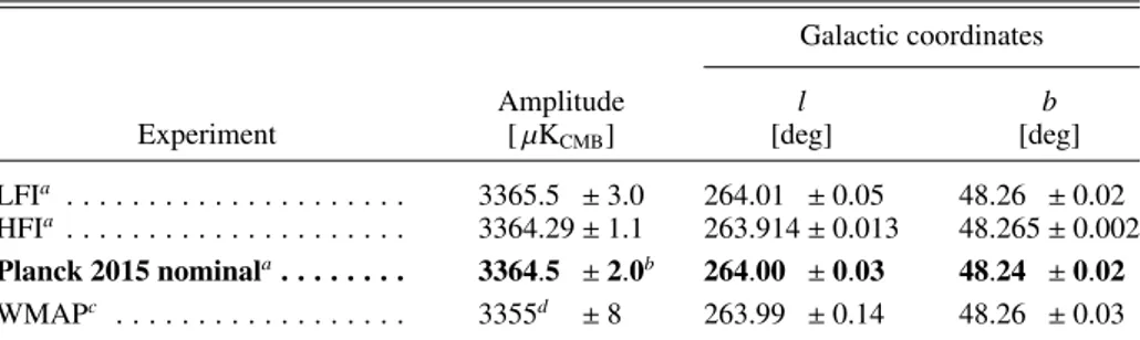
Table 1. LFI, HFI, and WMAP measurements of the Solar dipole.
Galactic coordinates
Amplitude l b
Experiment [ µKCMB] [deg] [deg]
LFIa . . . . 3365.5 ± 3.0 264.01 ± 0.05 48.26 ± 0.02
HFIa . . . . 3364.29 ± 1.1 263.914 ± 0.013 48.265 ± 0.002
Planck 2015 nominala. . . . 3364.5 ± 2.0b 264.00 ± 0.03 48.24 ± 0.02
WMAPc . . . . 3355d ± 8 263.99 ± 0.14 48.26 ± 0.03
Notes.(a)The “nominal” Planck dipole was chosen as a plausible combination of the LFI and HFI measurements early in the analysis, to carry out
subtraction of the dipole from the frequency maps (see Sect.5.4.3). The current best determination of the dipole comes from an average of 100 and 143 GHz results (Planck Collaboration VIII 2016).(b)Uncertainties include an estimate of systematic errors.(c)Hinshaw et al.(2009).(d)See
Sect.5.4.1for the effect of this amplitude on Planck calibration in 2013.
Table 2. LFI calibration changes at map level, 2013 → 2015.
Beam solid Pipeline Orbital
Frequency angle improvementsa dipoleb Total
[GHz] [%] [%] [%] [%]
30 . . . +0.32 −0.15 +0.28 +0.45 44 . . . +0.03 +0.33 +0.28 +0.64 70 . . . +0.30 +0.24 +0.28 +0.82 Notes. (a) This term includes the combined effect of the new
destrip-ing code, subtraction of Galactic contamination from timelines, and a new gain smoothing algorithm. It has been calculated under the sim-plifying assumption that it is fully independent of the beam convolu-tion.(b)Change from not being dependent on the amplitude error of the
WMAP9 Solar dipole (Sect.5.4.1).
and orbital dipoles, including their induced frequency indepen-dent quadrupoles) is performed with the full 4π beam rather than a pencil beam. This dipole model is used to extract the gain calibration parameter. Because the details of the beam pat-tern are unique for each detector even within the same fre-quency channel, the reference signal used for the calibration is different for each of the 22 LFI radiometers. This change im-proves the results of null tests and the quality of the polarization maps. When taking into account the proper window functions (Planck Collaboration IV 2016), the new convolution scheme leads to shifts of+0.32, +0.03, and +0.30% in gain calibration at 30, 44, and 70 GHz, respectively (see Table 2). Second, a new destriping code, Da Capo (Planck Collaboration V 2016), is used; this supersedes the combination of a dipole-fitting rou-tine and the Mademoiselle code used in the 2013 data release and offers improved handing of 1/ f noise and residual Galac-tic signals. Third, GalacGalac-tic contamination entering via sidelobes is subtracted from the timelines after calibration. Finally, a new smoothing algorithm is applied to the calibration parameters. It adapts the length of the smoothing window depending on a num-ber of parameters, including the peak-to-peak amplitude of the dipole seen within each ring and sudden temperature changes in the instrument. These changes improve the results of null tests, and also lead to overall shifts in gain calibration a few tenths of a percent, depending on frequency channel. The values reported in the third column of Table2are approximate estimates from the combination of improved destriping, Galactic contamination re-moval, and smoothing. They are calculated under the simplifying assumption that these effects are completely independent of the
beam convolution and can therefore be combined linearly with the latter (for more details seePlanck Collaboration V 2016).
In total, these four improvements give an overall increase in gain calibration for LFI of+0.17, +0.36, and +0.54% at 30, 44, and 70 GHz, respectively. Adding the 0.28% error introduced by the WMAP Solar dipole in 2013 (discussed in Sect.5.4.1), for the three LFI frequency channels we find overall shifts of about 0.5, 0.6 and 0.8% in gain calibration with respect to our LFI 2013 analysis (see Table2).
As shown in Planck Collaboration V (2016), relative cali-bration between LFI radiometer pairs is consistent within their statistical uncertainties. At 70 GHz, using the deviations of the calibration of single channels, we estimate that the relative cali-bration error is about 0.1%.
HFI – There were three significant changes related to HFI cali-bration between the 2013 and the 2015 results: improved deter-mination and handling of near and far sidelobes; improved ADC nonlinearity correction; and improved handling of very long time constants. The most significant changes arise from the introduc-tion of near sidelobes of the main beam in the range of angles 0.◦5 to 5◦, and from the introduction of very long time constants.
We consider these in turn.
Observations of Jupiter were not used in the 2013 results, because its signal is so strong that it saturates some stages of the readout electronics. The overall transfer function for each detector is corrected through the deconvolution of a time trans-fer function, leaving a compact effective beam that is used to-gether with the maps in the science analysis. In the subsequent “consistency paper” (Planck Collaboration XXXI 2014), it was found that lower-noise hybrid beams built using observations of Mars, Saturn, and Jupiter reveal near sidelobes leading to signif-icant corrections of 0.1 to 0.3%. Far sidelobes give a very small calibration correction that is almost constant for ` > 3. The zodi-acal contribution was removed in the timelines, since it does not project properly on the sky; it gives an even smaller and negli-gible correction except in the submillimetre channels at 545 and 857 GHz.
The most significant change results from the recognition of the existence of very long time constants (VLTC) and their in-clusion in the analysis. VLTCs introduce a significant shift in the apparent position of the dominant anisotropy in the CMB, the Solar dipole, away from its true position. This in effect cre-ates a leakage of the Solar dipole into the orbital dipole. This is the reason why calibration on the orbital dipole did not work as expected from simulations, and why calibration in 2013 was instead based on the WMAP5 Solar dipole. As discussed in
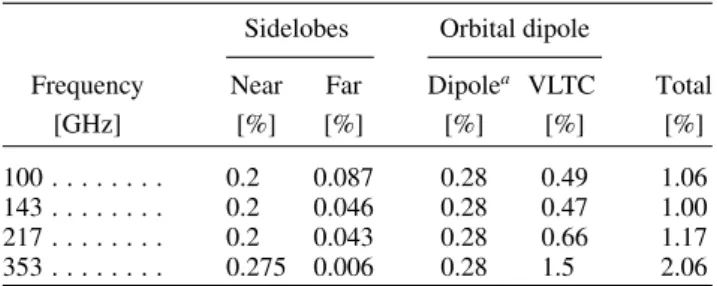
Table 3. HFI calibration changes at map level, 2013 → 2015.
Sidelobes Orbital dipole
Frequency Near Far Dipolea VLTC Total
[GHz] [%] [%] [%] [%] [%]
100 . . . 0.2 0.087 0.28 0.49 1.06
143 . . . 0.2 0.046 0.28 0.47 1.00
217 . . . 0.2 0.043 0.28 0.66 1.17
353 . . . 0.275 0.006 0.28 1.5 2.06
Notes.(a)Change from not being dependent on the amplitude error of
the WMAP9 Solar dipole (Sect.5.4.1).
Sect. 5.4.1, the WMAP5 Solar dipole was underestimated by 0.28% when compared with the Planck best-measured ampli-tude, leading to an under-calibration of 0.28% in the Planck 2013 maps. With VLTCs included in the analysis, calibration on the orbital dipole worked as expected, and gave more accurate re-sults, while at the same time eliminating the need to adopt the WMAP5 Solar dipole and removing the 0.28% error that it in-troduced in 2013.
These HFI calibration changes are summarized in Table3. Together, they give an average shift of gain calibration of typ-ically 1% (Planck Collaboration VIII 2016) for the three CMB channels, accounting for the previously unexplained difference in calibration on the first acoustic peak observed between HFI and WMAP.
The relative calibration between detectors operating at the same frequency is within 0.05% for 100 and 143 GHz, 0.1% at 217 GHz, and 0.4% at 353 GHz (Planck Collaboration VIII 2016). These levels for the CMB channels are within a factor of 3 of the accuracy floor set by noise in the low-` polarization (Tristram et al. 2011).
The 545 and 857 GHz channels are calibrated separately using models of planetary atmospheric emission. As in 2013, we used both Neptune and Uranus. The main difference comes from better handling of the systematic errors affecting the planet flux density measurements. Analysis is now performed on the timelines, using aperture photometry, and taking into account the inhomogeneous spatial distribution of the samples. For the frequency maps, we estimate statistical errors on absolute cali-bration of 1.1% and 1.4% at 545 and 857 GHz, respectively, to which we add the 5% systematic uncertainty arising from the planet models. Errors on absolute calibration are therefore 6.1 and 6.4% at 545 and 857 GHz, respectively. Since the reported relative uncertainty of the models is of the order of 2%, we find the relative calibration between the two HFI high-end frequen-cies to be better than 3%. Relative calibration based on diffuse foreground component separation gives consistent numbers (see table 6 ofPlanck Collaboration X 2016). Compared to 2013, cal-ibration factors changed by 1.9 and 4.1% at 545 and 857 GHz, respectively. Combined with other pipeline changes (such as the ADC corrections), the brightness of the released 2015 frequency maps has decreased by 1.8 and 3.3% compared to 2013. 5.4.3. Relative calibration and consistency
The relative calibration of LFI, HFI, and WMAP can be assessed on several angular scales. At ` = 1, we can compare the ampli-tude and direction of the Solar dipole, as measured in the fre-quency maps of the three instruments. On smaller scales, we can
compare the amplitude of the CMB fluctuations measured fre-quency by frefre-quency by the three instruments, during and after component separation.
– Comparison of independent measurements of the Solar dipole. Table1gives the LFI and HFI measurements of the Solar dipole, showing agreement well within the uncertainties. The ampli-tudes agree within 1.2 µK (0.04%), and the directions agree within 40. Table1 also gives the “nominal” Planck dipole that has been subtracted from the Planck frequency maps in the 2015 release. This is a plausible combination of the LFI and HFI val-ues, which satisfied the need for a dipole that could be subtracted uniformly across all Planck frequencies early in the data pro-cessing, before the final systematic uncertainties in the dipole measurements were available and a rigorous combination could be determined. See Planck Collaboration VIII(2016) Sect. 5.1 for additional measurements.
Nearly independent determinations of the Solar dipole can be extracted from individual frequency maps using component-separation methods relying on templates from low and high fre-quencies where foregrounds dominate (Planck Collaboration V 2016;Planck Collaboration VIII 2016). The amplitude and di-rection of these Solar dipole measurements can be compared with each other and with the statistical errors. This leads to relative gain calibration factors for the ` = 1 mode of the maps expressed in KCMB units, as shown for frequencies from
70 to 545 GHz in Table 4. For components of the signal with spectral distribution different from the CMB, a colour correc-tion is needed to take into account the broad bands of these experiments.
– Comparison of the residuals of the Solar dipole left in the CMB maps after removal of the best common estimate.Another mea-surement of relative calibration is given by the residuals of the Solar dipole left in CMB maps after removing the best com-mon estimate, i.e., the nominal Planck dipole. (See Sects. 4 and5.4.1for details about how the dipole and quadrupole are handled.) The residual dipole comes from two terms, as illus-trated in Fig.5, one associated with the error in direction, with an axis nearly orthogonal to the Solar dipole, and one associ-ated with the error in amplitude aligned with the Solar dipole. Using the 857 GHz map as a dust template (extrapolated with optimized coefficients derived per patch of sky), we find residual dipoles dominated by errors orthogonal to the direction of the Solar dipole at 100 and 143 GHz, and residuals associated with calibration errors for the other frequencies. The relative residual amplitudes are given in Table4. This shows that a minimization of the dipole residuals can and will be introduced in the HFI cal-ibration pipeline for the final 2016 release.
– Comparison of CMB anisotropies frequency by frequency during and after component separation. Table 4 also shows the relative calibration between frequencies and de-tectors determined by SMICA (Planck Collaboration XV 2014; Planck Collaboration IX 2016) and Commander (Planck Collaboration IX 2016; Planck Collaboration X 2016), two of the map-based diffuse component-separation codes used by Planck. The calculation is over different multipole ranges for the two methods, so variation between the two could reflect uncertainties in transfer functions. Moreover, Commander uses different constraints in order to deal with the complexities and extra degrees of freedom involved in fitting foregrounds indi-vidually (see Planck Collaboration X 2016 for details), so we do not expect identical results with the two codes. Nevertheless, the agreement is excellent, at the 0.2% level between the first