A stochastic volatility framework with analytical
filtering
Giacomo Bormetti, Roberto Casarin, Fulvio Corsi and Giulia Livieri
Abstract Motivated by the fact that realized measures of volatility are affected by measurement errors, we introduce a new family of discrete-time stochastic volatility models having two measurement equations relating both the observed returns and realized measures to the latent conditional variance.
Key words: Bayesian Inference, Monte Carlo Markov Chain, High-frequency, Re-alized volatility, ARG, Stochastic volatility
1 Introduction
In this paper we introduce a new family of discrete-time Stochastic Volatility (SV) models, for the joint modelling of returns and realized measures of volatility. The proposed model is characterized by having two measurement equations for the latent volatility: (i) a Normal density for the daily returns and (ii) a Gamma density for the RV measure. We then term the general version of the proposed model as SV-ARG. A salient feature of the SV-ARG is that it allows for analytical filtering and smoothing recursions for the latent factor that guides the dynamics of daily returns. This permits us to develop an effective Bayesian inference procedure for both parameters and latent factor.
Giacomo Bormetti
University of Bologna, e-mail: [email protected] Roberto Casarin
University Ca’ Foscari of Venice, e-mail: [email protected] Fulvio Corsi
University Ca’ Foscari of Venice, e-mail: [email protected] Giulia Livieri
Scuola Normal Superiore, Pisa, e-mail: [email protected]
205 Alessandra Petrucci, Rosanna Verde (edited by), SIS 2017. Statistics and Data Science: new challenges, new generations. 28-30 June 2017 Florence (Italy). Proceedings of the Conference of the Italian Statistical Society
2 The model
Consider a financial log-return process rt, a realized variance process yt and a latent
volatility process ht. Let Ft=. σ (rt,yt)be theσ-algebra containing the information
about observable quantities (log-return and realized variance yt) available at time t,
and !FtH =. σ (Ft−1,ht). We assume the following model for the dynamics of the
log-returns:
rt =µ + γht+"htεt, εt i.i.d.∼ N (0,1), (1)
t = 1,...,T , whereµ is the risk-free rate and γ is the market price of risk. N (m,σ2)
indicates the univariate normal distribution with mean m and varianceσ2. The
dy-namics in Equation (1) differs from that employed in Corsi et al. (2013); Majewski et al. (2015) for daily log-returns inasmuch in these works authors consider as driv-ing process for returns a realized measure of volatility. Specifically, they employ the continuous part of the realized variance, hereafter RV, defined as the sum of squared returns over non-overlapping intervals within a sampling period. We refer to Equation (1) as return equation.
Since the RV contains information on the latent volatility process, we follow au-thors in Hansen and Lunde (2006); Engle and Gallo (2006); Shephard and Sheppard (2010); Takahashi et al. (2009) and introduce another measurement equation, termed realized variance equation, which relates the observed RV to the latent process ht.
Specifically, we assume that the realized variance yt is sampled from a Gamma
dis-tribution
yt| !FtH i.d.∼ G (α,ht) , (2)
where α ∈ R+ is constant. In the previous equation, G (k,ϑ) denotes a Gamma
distribution with positive shape, k, and scale parameter,ϑ.
We assume that ht follows an autoregressive gamma process with transition
distri-bution (see Gouri´eroux and Jasiak, 2006):
ht| !Ft−1H ,rt−1,yt−1∼ ¯d G (ν,φcht−1,c). (3)
In the previous equation, ¯G (ν,φcht−1,c) denotes the non-central gamma distribution
with shapeν > 0, scale c > 0 and non-centrality φcht−1. Using the Poisson mixture
representation for the non-central gamma distribution (see Gouri´eroux and Jasiak, 2006, for more details), we rewrite Equation (3) as
ht|zt i.d∼ G (ν + zt,c),
zt|ht−1i.d∼ P (ϕht−1) ,
where, in general, Po(v) indicates the Poisson distribution with intensity parameter v. The latter representation is useful for both the characterization of ht and the
function of this process and its risk neutral dynamics are given in (Bormetti et al., 2016).
3 Analytical filtering and smoothing
Applying similar argument as in Creal (2015), we are able to provide analytical expressions for the: (i) conditional likelihood, (ii) Markov transition, (iii) initial dis-tribution of zt, (iv) filtering and the smoothing of the latent process ht. In particular,
the following two propositions hold.
Proposition 1. For the SV-ARG model described in Equation (1), (2) and (3) the conditional likelihood, p(rt,yt|zt,θ), the Markov transition, p(zt|zt−1,rt−1,yt−1,θ),
and the initial distribution of zt, p(z1;θ), are respectively given by: p(rt,yt|zt;θ) = 2η(zt,yt;θ)Kλ(zt) !" ψχ(t)# ⎛ ⎝ & χ(t) ψ ⎞ ⎠ λ(zt) , p(zt|zt−1,rt−1,yt−1;θ) ∝ S ) λ(zt−1),χ(t−1)φ (d) c ,ψ c φ(d) * , p(z1;θ) ∝ N B + ν,φ(d),, with η(zt,yt;θ) =exp(γµ√ 1t) 2π yαt−1 t Γ (αt) 1 Γ (ν + zt)cν+zt, µ1t=rt− µ, αt=α, λ(zt) =ν + zt− αt− 1/ 2, χ(t)=µ2 1t+2µ2t, µ2t=yt, ψ = γ2+2 c. Proof. See Bormetti et al. (2016).
Proposition 2. Let λ(zt),χ(t)andψ be the quantities defined in Proposition 1. The
marginal filtered, p(ht|r1:t,y1:t,z1:t,x1:t;θ), and smoothed, p(ht|r1:T,y1:T,z1:T,x1:T;θ)
distributions are p(ht|r1:t,y1:t,z1:t,x1:t;θ) ∝ G ig + λ(zt),χ(t),ψ , , p(ht|r1:T,y1:T,z1:T,x1:T;θ) ∝ G ig ) λ(zt) +zt+1,χ(t),ψ + 2φ (d) c * , t = 1,··· ,T.
4 Simulation results
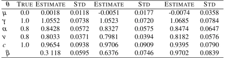
For the SV-ARG model we simulate 50 data-series of 1,000 observations. For each data-series we run the Gibbs sampler in Bormetti et al. (2016) for 100,000 itera-tions, discard the first 20,000 draws to avoid dependence from initial condiitera-tions, and finally apply a thinning procedure to reduce the dependence between consec-utive draws. We test the efficiency of the algorithm in three different scenarios:
LOW-PERSISTENCE(β = 0.3),MEDIUM PERSISTENCE(β = 0.6), and finally,HIGH PERSISTENCE(β = 0.9). The true values for the other parameters used in the
sim-ulations are reported in Table 1together with the grand average of the parameter posterior means along with their robust standard deviations. The results in Table 1 indicates the accuracy of the MCMC scheme is remarkable for all the scenarios (LOWPERSISTENCE, MEDIUM PERSISTENCE, HIGH PERSISTENCE). As regards
the efficiency, the magnitudes of the inefficiency factor after applying a thinning procedure are below ten.
Table 1 SUMMARY OUTPUT OF THE PARAMETER ESTIMATES FOR THESV-ARGMODEL
LOWPERSISTENCE MEDIUMPERSISTENCE HIGHPERSISTENCE
θ TRUEESTIMATE STD ESTIMATE STD ESTIMATE STD
µ 0.0 0.0018 0.0118 -0.0051 0.0177 -0.0074 0.0358 γ 1.0 1.0552 0.0738 1.0523 0.0720 1.0685 0.0784 α 0.8 0.8428 0.0572 0.8327 0.0575 0.8474 0.0647 ν 0.8 0.8033 0.0371 0.7981 0.0394 0.8182 0.0576 c 1.0 0.9654 0.0938 0.9706 0.0909 0.9395 0.0790 β 0.3 118 0.0595 0.6376 0.0746 0.9702 0.0839
5 Conclusions
Motivated by the presence of measurement errors in the empirically computed re-alized volatility measures we introduce a new family of discrete-time models. We derive the analytical filtering and smoothing and show that they can be used for efficient inference on the parameters and the latent volatility process.
Acknowledgements All authors warmly thank Drew D. Creal for helpful comments on the imple-mentation of the algorithm for computing the Bessel function of the second kind and Dario Alitab for support during the development of the pricing code. The research activity of RC is supported by funding from the European Union, Seventh Framework Programme FP7/2007-2013 under Grant agreement FP7/2007-2013, and by the Italian Ministry of Education, University and Research (MIUR) PRIN 2010-11 Grant MISURA. GL acknowledges research support from the Scuola Normale Superiore Grant SNS_14_BORMETTI and CI14_UNICREDIT_MARMI. This research used the SCSCF multiprocessor cluster system at University Ca’ Foscari of Venice.
References
Bormetti, G., Casarin, R., Corsi, F., and Livieri, G. (2016). Smiles at errors: A discrete-time stochastic volatility framework for pricing options with realized measures. Working Paper, University Ca’ Foscari of Venice.
Chib, S., Nardari, F., and Shephard, N. (2002). Markov chain Monte Carlo methods for stochastic volatility models. Journal of Econometrics, 108(2):281–316. Corsi, F., Fusari, N., and La Vecchia, D. (2013). Realizing smiles: Options pricing
with realized volatility. Journal of Financial Economics, 107(2):284–304. Creal, D. D. (2015). A class of non-Gaussian state space models with exact
likeli-hood inference. Journal of Business & Economic Statistics, (just-accepted). Engle, R. F. and Gallo, G. M. (2006). A multiple indicators model for volatility
using intra-daily data. Journal of Econometrics, 131(1):3–27.
Gouri´eroux, C. and Jasiak, J. (2006). Autoregressive gamma processes. Journal of Forecasting, 25(2):129–152.
Hansen, P. R. and Lunde, A. (2006). Realized variance and market microstructure noise. Journal of Business & Economic Statistics, 24(2):127–161.
Majewski, A. A., Bormetti, G., and Corsi, F. (2015). Smile from the past: A gen-eral option pricing framework with multiple volatility and leverage components. Journal of Econometrics, 187(2):521–531.
Shephard, N. and Sheppard, K. (2010). Realising the future: Forecasting with high-frequency-based volatility (HEAVY) models. Journal of Applied Econometrics, 25(2):197–231.
Takahashi, M., Omori, Y., and Watanabe, T. (2009). Estimating stochastic volatility models using daily returns and realized volatility simultaneously. Computational Statistics & Data Analysis, 53(6):2404–2426.