Dynamic Interactions among Growth, Environmental Change, Habit Formation, and Preference Change

DYNAMIC INTERACTIONS AMONG

GROWTH, ENVIRONMENTAL CHANGE,

HABIT FORMATION, AND PREFERENCE

CHANGE

WEI-BIN ZHANG

Ritsumeikan Asia Pacific University, Japan

Received: March 27, 2013 Accepted: July 30, 2013 Online Published: October 10, 2013

Abstract

The purpose of this study is to construct an economic growth model with environmental change and preference formation. The paper is focused on dynamic interactions among capital accumulation, environmental change, habit formation, preference change, and division of labor in perfectly competitive markets with environmental taxes on production, wealth income, wage income and consumption. The model integrated the dynamic economic mechanisms in the neoclassical growth theory, the environmental dynamics in traditional models of environmental economics, and the literature of economic growth with habit formation and within a comprehensive framework. It is showed that the motion of the economic system is given by three nonlinear autonomous differential equations. We simulate the time-invariant system. The simulation demonstrates some dynamic interactions among the economic variables which can be predicted neither by the neoclassical growth theory nor by the traditional economic models of environmental change. For instance, if the past consumption has weaker impact on the current consumption, although the long-term equilibrium of the dynamic system will not be affected, the transitional paths are shifted as follows: initially the transitional path of the stock habit becomes lower than its original path; the consumption level falls initially in association with falling in the propensity to consume; the exogenous disturbance causes the propensity to consume to fall and the propensity to save to rise; the national wealth and capital inputs of the two sectors are augmented; the labor force is shifted initially from the industrial sector to the environmental sector, but subsequently the direction is opposite before the labor distribution comes to its original equilibrium point; the wage rate is enhanced in association with falling in the rate of interest; the level of pollution falls initially, but rise subsequently; the output levels of the two sectors and the total tax income are enhanced before they come back to their original paths.

Keywords: Habit formation; preference change; environmental tax; pollution; economic growth.

Acknowledgements: The author is grateful for the financial support from the Grants-in-Aid for Scientific Research (C), Project No. 25380246, Japan Society for the Promotion of Science.

1. Introduction

Economic growth has close relationships with environmental changes. As far as neoclassical growth theory is concerned, early formal modeling on tradeoffs between consumption and pollution were found in the seminal papers by Plourde (1972) and Forster (1973). Interactions between environmental change and economic growth have received increasingly attention in the literature of economic growth and development (see, for instance, Pearson, 1994; Grossman, 1995; Copeland and Taylor, 2004; Stern 2004; Brock and Taylor, 2006; Dasgupta, et al. 2006). In the literature of economic development and environmental change many researches are conducted to confirm or question the environmental Kuznets curve. The environmental Kuznets curve refers to the phenomenon that per capita income and environmental quality follow an inverted U-curve. A recent survey on the literature of the curve is given by Kijima et al. (2010). In fact, in the increasing literature of empirical studies on relations between growth and environmental quality rather than the suggested environmental Kuznets curve one finds different relations such as inverted U-shaped relationship, a U-shaped relationship, a monotonically increasing or monotonically decreasing relationship (Dinda, 2004; Managi, 2007; Tsurumi and Managi, 2010). The various relations between economic development and environmental quality the inability of economic theories for properly explaining these observed phenomena implies the necessity that more comprehensive theories are needed. The purpose of this study is to introduce habit formation and preference change into the literature of economic growth and environmental change. As far as I am aware, there is no formal neoclassical growth model based on micro economic foundation which deals with economic growth, environmental change, habit formation, and preference change in an integrated framework.

People behave under influences of their habits. These habits are formed over years. People may change their habits with different speeds. Habits are parts of preferences. Different people have different preferences. The preference is also changeable over time for the same person. This study tries to integrate habit formation, preference change and economic growth within a comprehensive framework. Preferences are changeable and many factors may attribute to these changes. For instance, Becker and Mulligan (1997) found that expenditures in health and education have positive impacts saving (see also, Fuchs, 1982; Shoda et al., 1990; Olsen, 1993; Kirby et al. 2002; Chao et al., 2009). Many empirical studies identify relations between preference changes and other changes in social and economic conditions (e.g., Horioka, 1990; Sheldon, 1997, 1998). In the literature of economic growth with preference change, economists analyze preference change mainly by introducing time preference change in the Ramsey growth model. A main approach to modeling relations between growth and preference change is the so-called endogenous time preference. The formal modeling in continuous time formation was initiated with Uzawa’s seminal paper (Uzawa, 1968). Following Uzawa, Lucas and Stokey (1984) and Epstein (1987) establish relations between time preference and consumptions. Becker and Barro (1988) build a time preference change model in which the parent’s generational discount rate is connected to their fertility. There are other studies on the implications of endogenous time preference for the macroeconomy (see, e.g., Epstein and Hynes, 1983; Obstfeld, 1990; Shin and Epstein, 1993; Palivos et al., 1997; Drugeon, 1996, 2000; Stern, 2006; Meng, 2006; Dioikitopoulos and Kalyvitis, 2010). The idea of analyzing change in impatience in this study is influenced by the literature of time preference. We introduce changes in impatience in an alternative utility proposed by Zhang (1993). Except the literature on time preference change, this study is also influenced by the so-called habit formation or habit persistence model. The model was initially proposed in formal economic analysis by Duesenberry (1949). Becker (1992) explains the role of habit in affecting human behavior as follows: “the habit acquired as a child or young adult generally continue to influence behavior even when the environment

changes radically. For instance, Indian adults who migrate to the United States often eat the same type of cuisine they had in India, and continue to wear the same type clothing.” Habit formation is also applied to different fields of economic analysis (for instance, Pollak, 1970; Mehra and Prescott, 1985; Sundaresan, 1989; Constantinides, 1990; Campbell and Cochrane, 1999; de la Croix, 1996; Boldrin et al., 2001; Christiano et al. 2005; Ravn et al., 2006; Huang, 2012). It should be noted that since the research by Abel (1990), ‘catching up with the Joneses’ is often used exchangeable with external habit formation.

The purpose of this paper is to study economic growth with environmental change and preference change on the basis of the Solow one-sector growth model, Zhang’s approach to household behavior, the neoclassical growth models with environmental change, the literature of time preference and the literature of habit formation. The model in this paper is an extension of Zhang’s two models on environmental change and habit formation. The interdependence between savings and dynamics of environment is mainly based on Zhang (2011), while the habit formation and preference change are based on Zhang (2012). Section 2 introduces the basic model with wealth accumulation, environmental dynamics, habit formation and preference change. Section 3 studies dynamic properties of the model and simulates the model, identifying the existence of a unique equilibrium and checking the stability conditions. Section 4 conducts comparative dynamic analysis with regard to some parameters. Section 5 concludes the study. The appendix proves the analytical results in Section 3.

2. The Basic Model

The production side of the economy consists of one industrial sector and one environmental sector. The industrial sector is similar to the standard one-sector growth model (see Burmeister and Dobell 1970; Barro and Sala-i-Martin, 1995). The economy has only one (durable) good and one pollutant in the economy under consideration. In the literature of environmental economics, there are different kinds of environmental variables (e.g., Moslener and Requate, 2007; Repetto, 1987; Leighter, 1999; and Nordhaus, 2000). Capital of the economy is owned by the households who distribute their incomes to consume the commodity and to save. Exchanges take place in perfectly competitive markets. The population N is fixed and homogenous. The labor force is fully employed by the two sectors. The commodity is selected to serve as numeraire (whose price is normalized to 1), with all the other prices being measured relative to its price. The industrial sector

Economic productivities are affected by pollution through different channels. For instance, pollution may directly affect production technology or the productivity of any input (Grimaud, 1999; Chao and Peck, 2000; Gradus and Smulders, 1996; Ono, 2002) for the impact on the productivity of any input. We assume that production is to combine labor force, Ni

( )

t , and physical capital, Ki

( )

t . We add environmental impact to the conventional production function. The production function is specified as follows

( )

= _iΓ_i

( ) ( ) ( )

( )

_{i i} , _i, _i, _i >0, _i + _i =1,

i t A E t K t N t A

F αi βi α β α β ₍₁₎ where Fi

( )

t is the output level of the industrial sector at time t, Γi

( )

E is a function of the environmental quality measured by the level of pollution, E

( )

t , A is the total productivity, and _i

i

α

and

β

_i are respectively the output elasticities of capital and labor. The environmental impact on the productivity Γ_i

( )

E is specified as follows

( )

( )

=

( )

, ≤0. Γ i b i E t E t b i

In perfectly competitive markets are competitive, labor and capital earn their marginal products. The environmental quality is not decided by any individuals firm. Let r

( )

t and w

( )

t

represent respectively the rate of interest and wage rate as follows

( )

(

1

_{( )}

) ( )

,

( )

(

1

_{( )}

) ( )

, t N t F t w t K t F t r i i i i i i i i k

τ

β

τ

α

δ

= − = − + (2) where

δ

k is the fixed depreciation rate of physical capital and

τ

i is the fixed tax rate,

. 1 0<<

τ

i <

Consumer behaviors

The representative household decides how much to consume and how much to save. This applies the approach to behavior of the household proposed by Zhang (1993). Per capita wealth is denoted by k

( )

t . We have k

( )

t =K

( )

t / N, where is the total capital stock. The per capita disposable current income which is the sum of the interest payment r

( ) ( )

t k t and the wage payment w

( )

t after taxation is given by

( ) (

t 1

) ( ) ( ) (

r t k t 1

) ( )

wt ,

y = −

τ

_k + −

τ

_w

where

τ

_k and

τ

_w are respectively the tax rates on the interest payment and wage income. The per capita disposable income is

( ) ( ) ( )

. ˆ t y t k t

y = + (3) The disposable income is distributed between saving and consumption. The representative household spends the total available budget on saving, s

( )

t , and the commodity, c

( )

t . The budget constraint is

(

1+

τ

_c

) ( ) ( ) ( )

ct + s t = yˆ t , (4) where

τ

_c is the tax rate on the consumption. In this study we neglect the possibility that consumers explicitly take care of environment. For modern economies, consumers tend to make efforts in improving environment, for instance, by preferring to environment-friendly goods. As observed by Selden and Song (1995), when society has a lower level of pollution, the representative agent may not care much about environment and spends his resource on consumption; however, as the environmental quality lowers and the agent earns more, the agent may spend more resources on environmental improvement.

The household decides the two variables, s

( )

t and c

( )

t . This study specifies the utility function as follows

( )

( )

_{( )}

( )

_{( )}

( )

_{( )}

_,

_{( ) ( )}

_{, , 0,} 0 0 0 0 0 0 > = ξ λ −χ _{ξ λ χ} t t t E t s t c t U t t t

where

ξ

₀

( )

t is the utility elasticity of the commodity, called the propensity to consume,

λ

₀

( )

t is the utility elasticity of saving, called the propensity to own wealth, and

χ

₀ is the elasticity of environmental quality. This type of utility function was initially proposed by Zhang (1993). As Balcao (2001) and Nakada (2004), we assume that utility is negatively to pollution, which is a side product of the production process. According to Munro (2009: 43), “environmental economics has been slow to incorporate the full nature of the household into its analytical structures. … [A]n accurate understanding household behavior is vital for environmental economics.” In our approach,

For the representative household, w(t) and r(t) are given in markets. Maximizing U(t) subject to (4) yields

( ) ( ) ( ) ( ) ( ) ( )

t t yˆ t , s t t yˆ t , c =

ξ

=

λ

(5) where

( )

( ) ( ) ( ) ( ) ( )

, ,

_{( )}

1

_{( )}

. 1 0 _{0 0} 0 t t t t t t t t c

ξ

λ

ρ

λ

ρ

λ

τ

ξ

ρ

ξ

+ ≡ ≡ + ≡

We call

ξ

( )

t and

λ

( )

t respectively the relative propensities to consume and to save. It is the values of the relative propensities, not the propensities, which matter in determining the expenditure allocation.

Dynamics of wealth accumulation

According to the definition of s

( )

t ,the change in the household’s wealth is given by

( ) ( ) ( )

t s t k t .

k& = − (6) The equation simply states that the change in wealth is equal to saving minus dissaving. The demand and supply balance

The output of the industrial sector equals the sum of the level of consumption, the depreciation of capital stock and the net savings. Hence we have

C

( ) ( )

t + S t − K

( )

t +

δ

kK

( )

t = Fi

( )

t , (7) where C

( ) ( )

t =c t N is the total consumption, and S

( )

t − K

( )

t +

δ

kK

( )

t is the sum of the net saving and depreciation, where S

( ) ( )

t ≡s t N.

Full employment of production factors

We use N t_e( ) and K t_e( ) to respectively stand for the labor force and capital stocks employed by the environmental sector. As full employment of labor and capital is assumed, we have

( )

t K

( )

t K

( )

t ,

Environmental change

We now describe dynamics of the stock of pollutants E

( )

t . Both production and consumption pollute environment. The dynamics of the stock of pollutants is specified as follows

( )

t F

( )

t C

( )

t Q

( )

t ₀E

( )

t ,

E& =

θ

_{f i} +

θ

_c − _e −

θ

(9) where q_f, q_c, and q₀ are positive parameters and

( )

= eΓe( ) e

( ) ( )

e , e, e, e >0,

e t A E K t N t A

Q αe βe α β ₍₁₀₎ where A_e,

α

_e,and

β

_e are positive parameters, and Γ_e(E) (≥0) is a function of E As in . Gutiérrez (2008), the emission of pollutants during production processes is linearly positively proportional to the output level. This is reflected by θf F in (10). As in John and Pecchenino (1994), John et al. (1995), and Prieur (2009), in consuming one unit of the good the quantity

θ

_c is left as waste. We consider

θ

_c is related to the technology and environmental sense of consumers. The term

θ

₀E is the rate that the nature purifies environment, where

θ

₀ is called the rate of natural purification. We use the term, e e ,

e e N

Kα β in Q_e to reflect that that the purification rate of environment is positively related to capital and labor inputs. The function Γ_e(E) means that the purification efficiency is related to the stock of pollutants. For simplicity, we specify Γ_e as follows

( )

be,

e e E =θ E

Γ where

θ

_e and b are parameters. _e The behavior of the environmental sector

In this study we consider that the environmental sector is financially supported by the government. The sector decides the number of labor force and the level of capital employed. The government’s tax revenue consists of the tax incomes on the industrial sector, consumption, wage income and wealth income. Hence, the government’s income is given by

( )

t F

( )

t C

( )

t Nw

( )

t r

( ) ( )

t K t .

Y_e =

τ

_{i i} +

τ

_c +

τ

_w +

τ

_k (11) As in Ono (2003), we assume that all the tax incomes are spent on environment. For simplicity, we assume that all the revenue of the government is spent on protecting environment. The environmental sector’s budget is

( )

(

r t +

δ

k

) ( )

Ke t + w

( ) ( )

t Ne t =Ye

( )

t . (12) According to Zhang (2011), the environmental sector employs labor and uses capital in such a way that the purification rate achieves its maximum under the given budget constraint. The sector’s optimal problem is given by

( )

t Q_e

Max s.t.:

(

r

( )

t +

δ

_k

) ( )

K_e t + w

( ) ( )

t N_e t =Y_e

( )

t . The optimal solution is

( )

where . , e e e e e e

β

α

β

β

β

α

α

α

+ ≡ + ≡

The time preference and the propensity to hold wealth

Following Zhang (2012), we introduce preference change through making the propensity to own wealth and propensity to consume endogenous variables. Zhang’s approach is influenced by the traditional approach to preference change in economic theory. To illustrate the approach in this study, we consider a traditional modeling framework by Chang et al. (2011) in which the representative household maximizes the following discounted lifetime utility with perfect foresight

( )

_, ( ) _,

0

∫

∞_{u c m e}−ρt _dt

in which u is the utility function, c is consumption, and m is holdings of real money balances. The time preference

ρ

( )

t is endogenously determined (see also, Uzawa, 1968; Epstein, 1987; Obstfeld, 1990; and Shi and Epstein, 1993). The variable changes as follows

( )

( )

( )

, 0

∫

∆ = t u s ds t

ρ

where ∆ >0 is an instantaneous subjective discount rate at time ,s which satisfies ∆'>0, ,

0 ">

∆ and ∆ −u∆'>0.We have

ρ

&

( )

t =∆

( )

u

( )

t .

There are many other studies with endogenous time preference (for instance, Dornbusch and Frenkel, 1973; Persson and Svensson, 1985; Blanchard and Fischer, 1989; Orphanides and Solow, 1990; Das, 2003; Hirose and Ikeda, 2008). Although this study does not follow the Ramsey approach in modeling behavior of household, we will adapt the ideas about time preference within the Ramsey framework. The time preference in the traditional approach is related to real wealth or/and current consumption. This study treats the propensity to save as a function of the wage rate and wealth. Following Zhang (2012), the dynamics of the propensity to save is

( )

( )

( )

,

0 t λ λwwt λkk t

λ = + + (14) where

λ

>0,

λ

w, and

λ

k are parameters. When

λ

w =

λ

k =0,

λ

0

( )

t is constant. If we follow

Uzawa’s idea, then it is reasonable to assume

λ

w >0 and

λ

k =0. If we follow the assumption that the rate of time preference is positively related to wealth, for instance, accepted by Smithin (2004) and Kam and Mohsin (2006), then

λ

w =0 and

λ

k > 0.

The habit formation and the propensity to consume

The modeling of the propensity to save is influenced by the literature of time preference change. In order to model how the propensity to consume, we will adapt the basic ideas in the habit formation approach to our framework. To illustrate the ideas in the traditional approach, we introduce the following habit formation (e.g., Alvarez-Cuadrado et al., 2004; and Gómez, 2008)

( )

= 0( )

_{( )}

1−

_{( )}

_, >_{0, 0}≤ ≤_1, ∞ − −

∫

ρ φ ρ φ φ s d s C s C e t t t s h h

where C

( )

t is the consumer’s consumption and C

( )

t is the economy-wide average consumption. A larger value for h implies that the household puts lower weights to more ₀

distant values of the levels of consumption. Taking the derivatives the equation with respect to time yields

( )

[

( )

1

( ) ( )

]

.

0 C s C s t

t h h

h& = φ −φ −

If φ =0, the habit formation corresponds to the model with external habits. If φ =1, the habit formation corresponds to the model with internal habits. If 0<φ <1, habits arise from both the consumer’s and average past consumption. There are other models with habit formation (Deaton and Muellbauer, 1980; Carroll, 2000; Fuhrer, 2000; Kozicki and Tinsley, 2002; Amano and Laubach, 2004; Carroll et al., 1997; Corrado and Holly, 2011). Following Zhang (2012), this study also applies the concept of habit stock to analyze how the past consumption affects the current preference. The habit formation is specified as

( )

t h₀

[

c

( ) ( )

t h t

]

.

h& = − ₍₁₅₎

Equation (15) corresponds to the model with internal habits. If the current consumption is higher than the level of the habit stock, then the level of habit stock will rise, and vice versa. The propensity to consume is relate to the habit stock as follows

( )

( )

( )

,

0 t ξ ξwwt ξhht

ξ = + + (16) where

ξ

>0,

ξ

w and

ξ

h ≥ 0 are parameters. If

ξ

w =0 and

ξ

h = 0,

ξ

0

( )

t is constant. The term

( )

t y w

ξ

implies that the propensity to consume is affected by the wage rate. If

ξ

w >(<) 0, then a rise in the wage rate enhances (lowers)

ξ

0

( )

t . It is reasonable to assume

ξ

w ≥0. The term

( )

t hh

ξ

shows that if h

( )

t _{rises, the propensity to consume will rise, and vice versa.} We have thus built the dynamic model. We now examine dynamics of the model.

3. The Motion of the Economic System

The appendix confirms that the motion of the economic system is given by three autonomous differential equations with z

( ) ( )

t _,ht _{and E}

( )

_{t . as the variables, where z}

( )

_{t is a new variable} defined by

( )

_{( )}

( )

. k t r t w t z δ + ≡

The following lemma shows that once we solve the time-invariant system, we know the values of all the other variables in the economy at any point of time.

Lemma 1

The motion of the three variables, z

( ) ( )

t _,ht _{and E}

( )

_{t , is obtained by solving the following} three autonomous differential equations with

z&

( )

t =Λ_z

(

z

( ) ( ) ( )

t ,ht ,Et

)

, h&

( )

t =Λ_c

(

z

( ) ( ) ( )

t ,h t , E t

)

, E

( )

t E

(

z

( ) ( ) ( )

t ,h t , E t

)

,

& _=Λ

(17) in which Λ_z, Λc, and ΛE are functions of z

( ) ( )

t ,ht and E

( )

t defined in the appendix. All the other variables are solved as functions of z

( ) ( )

t _,ht _{and E}

( )

_{t as follows: r}

( )

_{t and w}

( )

_{t by (A2)}

→ ξ₀

( )

t by (A16) → λ₀

( )

t by (A15) → λ

( )

t and ξ

( )

t by (5) → K_i

( )

t and K_e

( )

t by (A7) →

( )

t K

( )

t K

( )

t

K = _i + _e → k

( )

t =K

( )

t /N → N_i

( )

t and N_x

( )

t by (A1) → F_i

( )

t by (1) → Q_e

( )

t

by (10) → yˆ

( )

t by (3) → c

( )

t and s

( )

t by (10).

From the procedure in Lemma 1 we can get the value of any variable at any point of time as functions of z

( ) ( )

t _,ht _{and E}

( )

_{t . The three dimensional autonomous differential equations are} nonlinear. It is almost impossible to get analytical solution of the time-invariant system. Nevertheless, we can use a common computer to follow the motion of the three-dimensional time-invariant system. To simulate the model, we choose the following parameter values

. 03 . 0 , 05 . 0 , 1 . 0 , 1 . 0 , 05 . 0 , 05 . 0 , 05 . 0 , 05 . 0 , 4 0 . 0 , 1 0 . 0 , 2 . 0 , 1 . 0 , 02 . 0 , 01 . 0 , 6 . 0 , 05 . 0 , 05 . 0 , 4 . 0 , 4 . 0 , 3 . 0 , 5 . 0 , 1 , 5 0 0 = = = = = = = = = = = = = − = = − = − = = = = = = = k c f w k c i h w k w e i e e i s i A b b A N

δ

θ

θ

θ

τ

τ

τ

τ

ξ

ξ

ξ

λ

λ

λ

β

α

α

h ₍₁₈₎

In the remainder of this study, the depreciation rate is fixed as δ_k =0.03. The population is chosen 10 and the total available time is unity. In our neoclassical model the population size has no impact on the per-capita variables, even though it affects the aggregate variable levels. The chosen values of the available time and the population will not affect our main conclusions. The total productivity and the output elasticity of capital of the capital goods sector are respectively 1.1, 0.35, and the total productivity and the output elasticity of capital of the capital goods sector are respectively 0.9 and 0.30. It should be noted that both in theoretical simulations and empirical studies the output elasticity of capital in the Cobb-Douglas production is often valued approximately equal to 0 and the value of the total productivity is .3 chosen to be close to unity (e.g., Miles and Scott, 2005; Abel, Bernanke, Croushore, 2007). Although the chosen values of the preference parameters are not empirically based, we choose the coefficients associated with the wage and wealth very small so that we may effectively analyze the effects of changes in these coefficients on the economic structure. We now specify the initial conditions to see how the variables change over time. To follow the motion of the system, we choose the following initial conditions:

( )

0 =6.5, _E

( )

0 =12, h

( )

0 =1.3. z

Figure 1 plots the simulation result. We first observe that the habit stock of leisure time falls while the habit stock of consumer goods rise till they respectively approach the leisure time and the consumption level of consumer goods. This happens as the two stocks are initially different from their corresponding variables. The work time, total labor supply and labor inputs of the two sectors are increased over time. The total capital and capital input of the consumer goods sector fall, while the capital input of the capital goods sector rises. The price and wage rate fall slightly, while the rate of interest rises. The propensity to consume rises, while the propensities to use leisure time and to save are affected only slightly. The GDP and the output level of the consumer goods sector fall while that of the capital goods sector rises. It should be noted that it takes much less time for the leisure time to converge to its habit stock level than the consumption level of consumer goods to its habit stock.

Figure 1 shows that the variables tend to move towards stationary states. This implies the existence of an equilibrium point. Our simulation identifies the equilibrium values of these variables as follows . 09 . 1 , 72 . 0 , 27 . 0 , 65 . 0 , 25 . 0 , 83 . 0 , 11 . 0 , 05 . 3 , 69 . 11 , 50 . 0 , 50 . 4 , 83 . 0 , 53 . 0 , 31 . 5 , 96 . 10 , 75 . 14 0 0 = = = = = = = = = = = = = = = = = c e i e i e e i c w r K K N N Y Q F E K h

λ

ξ

λ

ξ

It is straightforward to get the following three eigenvalues . 05 . 0 , 03 . 0 137 . 0 ± − − i

As the three eigenvalues have real negative parts, the equilibrium point is locally stable. Hence, the system always approaches its equilibrium if it is not far from the equilibrium point. This is important as it guarantees the validity of comparative dynamic analysis for transitional paths.

4. Comparative Dynamic Analysis

From the analysis in the previous section we know that that the economic system has a unique locally stable equilibrium. This guarantees that we can make comparative dynamic analysis. This section conducts comparative dynamic analysis with regard to some parameters. It should be remarked that because the system contains many variables which nonlinearly interact with each other in a very complicated manner over time, it is not easy to accurately interpret how all these variables interact over time.

Figure 1 – The Motion of the Economic System

Lower weights being put to more distant values of the levels of consumption

We first study the case where the household puts lower weights to more distant values of the levels of consumption in the following way: h₀:0.1⇒0.3. _{The rise in the parameter also} means that the habit stock and the current level of consumption mutually converge faster. Figure 2 diagrams the simulation results. In this study we use the variable ∆x

( )

t to stand for the change rate of the variable, x

( )

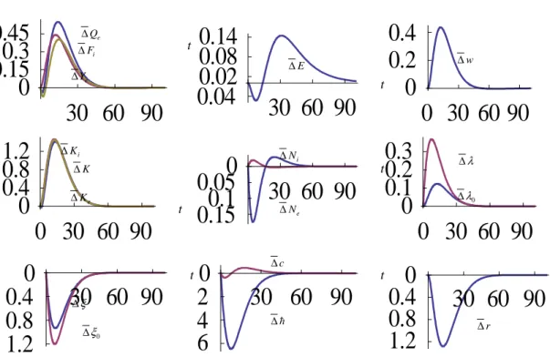
t , in percentage due to changes in some parameter value. Indeed, the disturbance in the speed of adjustment will not affect the equilibrium of the dynamic system. Nevertheless, the transitional paths towards the equilibrium points of the variables are strongly perturbed. As the household puts lower weights to more distant values of the levels of consumption, initially the transitional path of the habit stock is deviated from the original path. As the speed is sped up, the path of the stock habit becomes lower than its original path. As the habit stock becomes lower, the consumption level also falls initially in association with falling in the propensity to consume. The disturbance causes the propensity to consume to fall and the propensity to save to rise. As the relative propensity to save is λ increased, the national wealth is augmented. The disturbance in the national wealth enables the two sectors to employ more capital. The labor distribution path is also shifted. The labor force is shifted initially from the industrial sector to the environmental sector, but subsequently the direction is opposite before the labor distribution comes to its original equilibrium point. The wage rate is enhanced in association with falling in the rate of interest. The level of pollution falls initially, but rise subsequently. The output levels of the two sectors and the total tax income are enhanced before they come back to their original equilibrium levels.

The environmental tax rate on consumption being enhanced

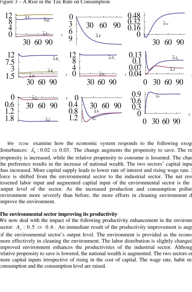
We now enhance the environmental tax rate on consumption as follows:

τ

_c: 0.05⇒0.07. The impacts are plotted in Figure 4. As the tax rate on consumption is increased, the consumption

25 50

75 100

12

13

14

15

25 50 75 100

11

11.3

11.6

11.9

0 25 50 75 100

0.82

0.83

0.84

0

25 50 75 100

3

4

5

0 25 50 75 100

0.72

0.78

0.82

0.86

0 25 50 75 100

0.5

0.55

0.6

0.65

25 50 75 100

1.1

1.2

1.3

25 50 75 100

0.255

0.26

0.265

0.27

25 50 75 100

0.1

0.104

0.108

h K 0 ξ λ r t t c t t t t t t t E i N e K i F e Y w e Q e N 0 λ ξ

Figure 2 – The Household Puts Lower Weights on More Distant Values of Consumption

level and the habit stock of consumption are lessened. The lowered habit stock diminishes the propensity to consumption, which implies augmenting in the propensity to save. The national wealth is increased as the propensity to save is increased. More capital and labor resources are located to the environmental sector. The environment is improved. Both the rate of interest and wage rate are increased. It should be noted that in the Solow-type neoclassical growth theory without endogenous environment, the rate of interest and wage rate are changed in the opposite directions. In our model the two variables are changed in the same direction because the environmental change affects the productivity. In our simulation case the improved environment augments the productivity of the industrial sector. This leads to the same change direction in the wage rate and the rate of interest. The net consequence of the rising national wealth and capital input of the environmental sector leads to lowering in the capital input of the industrial sector. As the capital and labor resources located to the industrial sector are lowered, the output level of the industrial sector is reduced.

Wealth more strongly affecting the propensity to save

How the propensity to save may influence economic growth and development is a main question in economics. It is well known that Adam Smith and Keynes have the opposite opinions about the effects of a change in the saving propensity. Adam Smith holds that a rise in the propensity to save will encourage long-run economic growth as to save more means more capital in the economy, while Keynes argues that to save less means to create more job opportunities and economic growth will be encouraged. In modern economics there is no convergence in empirical studies about the impact of the propensity to save. Moreover, there are only few formal models of economic growth with endogenous preference for saving. Our model explicitly introduces endogenous propensity to save.

30 60 90

0

0.15

0.3

0.45

30 60 90

0.04

0.02

0.08

0.14

0 30 60 90

0

0.2

0.4

0 30 60 90

0

0.4

0.8

1.2

30 60 90

0.15

0.1

0.05

0

0 30 60 90

0

0.1

0.2

0.3

30 60 90

1.2

0.8

0.4

0

30 60 90

6

4

2

0

30 60 90

1.2

0.8

0.4

0

t K ∆ h ∆ 0 ξ ∆ e Y ∆ c ∆ e K ∆ i K ∆ t t t t t t t t 0 λ ∆ i N ∆ E ∆ r ∆ w ∆ i F ∆ e Q ∆ e N ∆ λ ∆ ξ ∆

Figure 3 – A Rise in the Tax Rate on Consumption

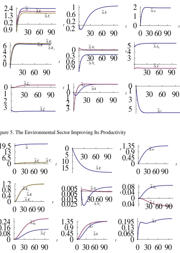
We now examine how the economic system responds to the following exogenous disturbances:

λ

k :0.02 ⇒ 0.03. The change augments the propensity to save. The relative propensity is increased, while the relative propensity to consume is lessened. The change in the preference results in the increase of national wealth. The two sectors’ capital inputs are thus increased. More capital supply leads to lower rate of interest and rising wage rate. Labor force is shifted from the environmental sector to the industrial sector. The net result of lessened labor input and augmented capital input of the environmental sector is the rising output level of the sector. As the increased production and consumption pollute the environment more severely than before, the more efforts in cleaning environment do not improve the environment.

The environmental sector improving its productivity

We now deal with the impact of the following productivity enhancement in the environmental sector: A_e : 0.5 ⇒ 0.6. An immediate result of the productivity improvement is augments of the environmental sector’s output level. The environment is provided as the economy is more effectively in cleaning the environment. The labor distribution is slightly changed. The improved environment enhances the productivities of the industrial sector. Although the relative propensity to save is lowered, the national wealth is augmented. The two sectors employ more capital inputs irrespective of rising in the cost of capital. The wage rate, habit stock of consumption and the consumption level are raised.

30 60 90

0

4

8

12

30 60 90

9

6

3

0

30 60 90

0

0.16

0.32

0.48

30 60 90

1.5

3

7.5

12

30 60 90

0

4

8

12

0 30 60 90

0.04

0.07

0.1

0.13

30 60 90

1.8

1.2

0.6

0

30 60 90

1.2

0.8

0.4

0

0 30 60 90

0

0.3

0.6

0.9

t K ∆ h ∆ 0 ξ ∆ e Y ∆ c ∆ e K ∆ i K ∆ t t t t t t t t 0 λ ∆ i N ∆ E ∆ r ∆ w ∆ i F ∆ e Q ∆ e N ∆ λ ∆ ξ ∆

Figure 4 – The Propensity to Save Being More Strongly Affected by Wealth

Figure 5. The Environmental Sector Improving Its Productivity

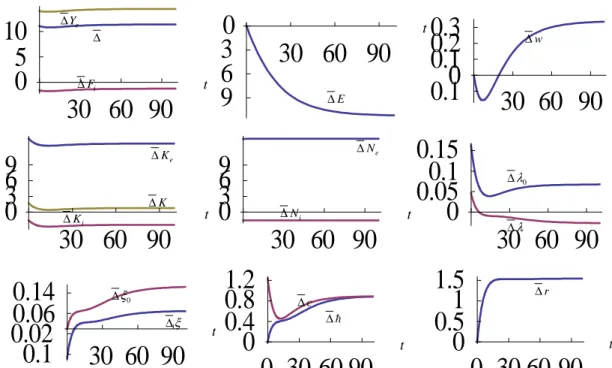
Raising the tax rate on the industrial sector

Let us now change the tax rate on the output level of the industrial sector as follows: . 07 . 0 05 . 0 : ⇒ i

τ

The raised tax rate lowers the output level of the industrial sector. As the tax revenue is increased, the environmental sector has more resources to employ more capital

30 60 90

0.9

0.2

1.3

2.4

30 60 90

0.2

0.2

0.6

1

0 30 60 90

0

1

2

30 60 90

0

2

4

6

30 60 90

0.9

0.6

0.3

0

30 60 90

3

4

5

30 60 90

3

2

1

0

30 60 90

3

2

1

0

1

30 60 90

5

3

1

0

0 30 60 90

0

6.5

13

19.5

30 60 90

15

10

5

0

0 30 60 90

0

0.45

0.9

1.35

0 30 60 90

0

0.4

0.8

1.2

30 60 90

0.025

0.015

0.005

0.005

30 60 90

0.04

0

0.04

0.08

0 30 60 90

0

0.08

0.16

0.24

0 30 60 90

0

0.45

0.9

1.35

0 30 60 90

0

0.065

0.13

0.195

t K ∆ h ∆ 0 ξ ∆ e Y ∆ c ∆ e K ∆ i K ∆ t t t t t t t t 0 λ ∆ i N ∆ E ∆ r ∆ w ∆ i F ∆ ∆ e N ∆ λ ∆ ξ ∆ t K ∆ h ∆ 0 ξ ∆ e Y ∆ c ∆ e K ∆ i K ∆ t t t t t t t t 0 λ ∆ i N ∆ E ∆ r ∆ w ∆ i F ∆ ∆ e N ∆ ∆λ ξ ∆

and labor inputs. The resources are shifted from the industrial sector to the environmental sector. The environment is improved. The industrial sector’s productivity is enhanced. As the productivity is enhanced only slightly in initial stage, the wage rate is reduced. As the productivity is further increased, the wage rate is increased. The reduced national wealth is associated with rising cost of capital. The relative propensity to save rises initially, but subsequently falls. The consumption level and habit stock of goods are increased.

Figure 6 – Raising the Tax Rate on the Industrial Sector

5. Concluding Remarks

The paper constructed an economic growth model with environmental change and preference formation. The paper is focused on dynamic interactions among capital accumulation, environmental change, habit formation, preference change, and division of labor in perfectly competitive markets with environmental taxes on production, wealth income, wage income and consumption. The model integrated the dynamic economic mechanisms in the neoclassical growth theory, the environmental dynamics in traditional models of environmental economics, and the literature of economic growth with habit formation and within a comprehensive framework. We could have synthesized the different ideas in a few main streams of economic theory as we applied an alternative approach to household behavior initially proposed by Zhang (1993). We showed that the motion of the economic system is given by three nonlinear autonomous differential equations. We simulated the time-invariant system.

The simulation demonstrates some dynamic interactions among the economic variables which can be predicted neither by the neoclassical growth theory nor by the traditional economic models of environmental change. For instance, we examined the effects that the household puts lower weights to more distant values of the levels of consumption. If the past consumption has weaker impact on the current consumption, although the long-term equilibrium of the dynamic system will not be affected, the transitional paths are shifted as follows: initially the transitional path of the stock habit becomes lower than its original path; the consumption

30 60 90

0

5

10

30 60 90

9

6

3

0

30 60 90

0.1

0

0.1

0.2

0.3

30 60 90

0

3

6

9

30 60 90

0

3

6

9

30 60 90

0

0.05

0.1

0.15

30 60 90

0.1

0.02

0.06

0.14

0 30 60 90

0

0.4

0.8

1.2

0 30 60 90

0

0.5

1

1.5

t K ∆ h ∆ 0 ξ ∆ e Y ∆ c ∆ e K ∆ i K ∆ t t t t t t t t 0 λ ∆ i N ∆ E ∆ r ∆ w ∆ i F ∆ ∆ e N ∆ λ ∆ ξ ∆

level falls initially in association with falling in the propensity to consume; the exogenous disturbance causes the propensity to consume to fall and the propensity to save to rise; the national wealth and capital inputs of the two sectors are augmented; the labor force is shifted initially from the industrial sector to the environmental sector, but subsequently the direction is opposite before the labor distribution comes to its original equilibrium point; the wage rate is enhanced in association with falling in the rate of interest; the level of pollution falls initially, but rise subsequently; the output levels of the two sectors and the total tax income are enhanced before they come back to their original paths.

As the model is based on the basic ideas in some economic theories, it is straightforward to extend the model in some directions. For instance, we may introduce leisure time as an endogenous variable. Munro (2009: 3) observes: “In the unitary model, the household acts as if it is a single individual maximizing a single utility function in the face of one budget constraint. It is a simplifying modeling assumption that is widely used in most branches of economics, but it is wrong. The fact that the unitary model is inaccurate is well-known and has been known for many years now.” It is necessary to model family structure and economic structure for understanding relations among growth, environmental change and preference change (see, for instance, Dinda, 2004; Hamilton and Zilberman, 2006).

Appendix: Identifying the Three Autonomous Differential Equations

We now find the three autonomous differential equations and confirm the procedure in the lemma. First, from (2) and (15), we solve

, e e e i i i N K N K z ≡ β = β (A1)

where

β

j ≡

β

j/

α

j, j =i,e. Substituting (1) into (2) yields

(

,

)

,

(

,

)

, i i i i i i i i k i i i i A z E z w z A E z r _α α β β

β

β

δ

β

α

Γ = − Γ = (A2) where we use (A1). From (8) and (A1), we solve

. N z K Ki e e i +β = β (A3) Insert (5) in (7)

(

ξ

+

λ

)

N yˆ − K +

δ

_kK =F_i. (A4) Put (3) in (A4)

(

)(

)

[

ξ

+

λ

τ

kr +1 −

δ

]

K +

(

ξ

+

λ

)

N

τ

ww= Fi, (A5) where

τ

_k ≡1−

τ

_k and

τ

_w ≡1−

τ

_w. Replacing F in (A5) with _i F_i =

(

r +

δ

_k

)

K_i/

α

_i

τ

_i from (2), we acquire

(

)(

)

[

1

]

(

)

(

)

. i i i k w k K r w N K r τ α δ τ λ ξ δ τ λ ξ + + − + + = + (A6) From K_i + K_e = K, (A6) and (A3), we solve

, , , _{i e} e i i e i K K K K N z K N K = = − = + ββ φ (A7) where

(

) (

₍

)

₎

(

) (

)

(

) (

)

(

)

(

,

)

[

(

)

/

]

. ~ , 1 1 , , 1 , , ~ , , , i e i i k k e i k w e k r E z r r E z w z r E z z E z

β

δ

β

τ

α

δ

δ

φ

τ

β

β

τ

φ

τ

β

τ

φ

φ

φ

λ

ξ

δ

φ

λ

ξ

λ

ξ

φ

ξ ξ ξ ξ ξ ξ − + + ≡ + − + ≡ + + ≡ + + − + ≡

From the definition of ξ and ,λ we have

, ~ 0 0 0 0 λ ξξ λ τ λ ξ + + = + (A8) where

τ

~≡1/

(

1+

τ

_c

)

. Insert (A8) in the definition of

φ

(

) (

₍

_~

)

₎

_~

₍

(

₎

)

. ~ , , , 0 0 0 0 0 0 0 0 0 0

λ

ξ

φ

φ

λ

ξ

τ

λ

ξ

δ

φ

λ

ξ

τ

λ

ξ

φ

ξ ξ ξ + + + + − + = z E z (A9) From (14), we acquire . 0 K N w N k w k +       ₊ =

λ

λ

λ

λ

λ

(A10)

Put (A7) in (A8)

, ~ 0 0

φ

β

φ

λ

= + (A11) where

(

,

)

, ~

(

)

. 0 e k i e e k w z w E z β λ β β β β λ λ λ φ = + + ≡ − (A12) Put (A9) in (A11)

(

)

(

)

(

_~

)

~

(

)

, ~ ~ ~ 0 0 0 0 0 0 0 0 0 0

λ

ξ

φ

φ

λ

ξ

τ

λ

ξ

δ

β

φ

β

λ

ξ

τ

φ

λ

ξ ξ ξ + + + + − + + = z (A13) We rewrite (A13) as follows

, 0 2 0 1 2 0 +ω λ −ω = λ (A14) where

(

)

(

)

_~ . ~ ~ ~ ~ ~ , , , ~ ~ ~ ~ ~ ~ , , 0 0 0 0 0 0 0 2 0 0 0 0 0 1 ξ ξ ξ ξ ξ ξ ξ ξ ξ ξ ξ ξ φ φ ξ φ β τ ξ δ β ξ φ φ φ φ ξ τ ξ ω φ φ φ β δ β φ φ φ φ ξ φ φ ξ τ ξ ω + + − + ≡ + − + − − + ≡ z E z z E z

We solve (A14) with

λ

0 as the variable

(

)

. 2 4 , , 2 2 1 1 0 0

ω

ω

ω

ξ

λ

z E = − ± + (A15) We have two solutions from the above equation. In our simulation case the solution

(

)

2 4 , , 2 2 1 1 0 0 0

ω

ω

ω

χ

ξ

λ

z = − + +

is meaningful. From (16), we have

(

, ,

)

.

0 z E h

ξ

ξ

ww

ξ

hh

ξ

= + + (A16) We solve all the variables as functions of ,z E and h as follows: r and w by (A2) → ,

ξ

0 by

(A16) →

λ

₀ by (A15) → λ and ξ by (5) → K_i and K_e by (A7) → K =K_i + K_e →

N K

k = / → N and _i N by (A1) _x → F by (1) _i → Q by (10)_e → yˆ by (3) → c and s by

(10). Here, we express the function for wealth obtained by this procedure as _k =Φ

(

_z, _E,h

)

. From (11), (3), (15) and (17) and the procedure to determine the variables as functions of ,z

,

E and ,h _{we have the following three differential equations}

(

z, E,

)

yˆ k, k&=Λ h ≡

λ

− _(A17)

(

z,E,

)

F C Q ₀E, E& =Λ_E h ≡

θ

_{f i} +

θ

_c − _e −

θ

(

z,E,

)

₀

[

c

( ) ( )

t t

]

. c h h h h & _{=Λ ≡ − (A18)}

We do not provide the expressions because they are tedious. Taking derivatives of

(

_{z, E,}h

)

, h & & ∂ Φ ∂ Λ + ∂ Φ ∂ Λ + ∂ Φ ∂ = E c E z z k (A19)

where we also apply (A18). Injecting (A17) in (A19) yields

(

, ,

)

. 1 −       ∂ Φ ∂       ∂ Φ ∂ Λ − ∂ Φ ∂ Λ − Λ ≡ Λ = z E E z z c c E z h h & _(A20)

We thus proved Lemma 1.

References

Abel, A. (1990). Asset Prices under Habit Formation and Catching up with the Joneses. American Economic Review, 80(2), 38-42.

Abel, A., Bernanke, B.S., & Croushore, D. (2007). Macroeconomics. New Jersey: Prentice Hall. Alvarez-Cuadrado, F., Monteriro, G., and Turnovsky, S.J. (2004). Habit Formation,

Catching-Up with the Joneses, and Economic Growth. Journal of Economic Growth, 9(1), 47-80. Amato, J.D., & Laubach, T. (2004). Implication of Habit Formation for Optimal Monetary

Policy. Journal of Monetay Economics, 51(2), 305-25.

Balcao, A. (2001). Endogenous Growth and the Possibility of Eliminating Pollution. Journal of Environmental Economics and Management, 42(3), 360-73.

Barro, R.J., & Sala-i-Martin, X. (1995). Economic Growth. New York: McGraw-Hill, Inc. Becker, G. (1992). Habits, Addictions and Traditions. Kyklos, 45(3), 327-45.

Becker, G.S., & Barro, R.J. (1988). A Reformation of the Economic Theory of Fertility. Quarterly Journal of Economics, 103(1), 139-71.

Becker, G.S., & Mulligan, C.B. (1997). The Endogenous Determination of Time Preference. The Quarterly Journal of Economics, 112(3), 729-58.

Blanchard, O.J., & Fischer, S. (1989). Lectures on Macroeconomics. Cambridge, MA: MIT Press.

Brock, W., & Taylor, M.S. (2006). Economic Growth and the Environment: A Review of Theory and Empirics, in S. Durlauf, & P. Aghion (Eds.), The Handbook of Economic Growth. Amsterdam: Elsevier.

Boldrin, M., Christiano, L., and Fisher, J. (2001). Habit Persistence, Asset Returns, and the Business Cycle. American Economic Review, 91(1), 149-66.

Burmeister, E., & Dobell, A.R. (1970). Mathematical Theories of Economic Growth. London: Collier Macmillan Publishers.

Campbell, J., & Cochrane, J. (1999). By Force of Habit: A Consumption-Based Explanation of Aggregate Stock Market Behavior. Journal of Political Economy, 107(2), 205-51.

Carroll, C.D. (2000). Solving Consumption Models with Multiplicative Habits. Economics Letters, 68(1), 67-77.

Carroll, C.D., Overland, J., & Weil, D.N. (1997). Consumption Utility in a Growth Model. Journal of Economic Growth, 2(4), 339-67.

Chang, W.Y., Tsai, H.F., & Chang, J.J. (2011). Endogenous Time Preference, Interest-Rate Rules, and Indeterminacy. The Japanese Economic Review, 62(3), 348-64.

Chao, H. and Peck, S. (2000). Greenhouse Gas Abatement: How Much? And Who Pays? Resource and Energy, 67(1), 1-24.

Chao, L.W., Szrek, H., Pereira, N.S., & Paul, M. (2009). Time Preference and Its Relationship with Age, Health, and Survival Probability. Judgment and Decision Making, 4(1), 1-19.

Christiano, L., Eichenbaum, M., & Evans, C. (2005). Nominal Rigidities and the Dynamic Effects of a Shock to Monetary Policy. Journal of Political Economy, 113(1), 1-45.

Constantinides, G. (1990). Habit Formation: A Resolution of the Equity Premium Puzzle. Journal of Political Economy, 98(3), 519-43.

Copeland, B., & Taylor, S. (2004). Trade, Growth and the Environment. Journal of Economic Literature, 42(1), 7-71.

Corrado, L., & Holly, S. (2011). Multiplicative Habit Formation and Consumption: A Note. Economics Letters, 113(2), 116-19.

Das, M. (2003). Optimal Growth with Decreasing Marginal Impatience. Journal of Economic Dynamics and Control, 27(10), 1881-98.

Dasgupta, S., Hamilton, K., Pandey, K.D., & Wheeler, D. (2006). Environment During Growth: Accounting for Governance and Vulnerability. World Development, 34(9), 1597-611.

De la Croix, D. (1996). The Dynamics of Bequeathed Tastes. Economics Letters, 51(1), 89-96. Deaton, A., & Muellbauer, J. (1980). Economics and Consumer Behavior. Cambridge:

Cambridge University Press.

Dinda, S. (2004). Environmental Kuznets Curve Hypothesis: A Survey. Ecological Economics, 49(4), 431-55.

Dioikitopoulos, E.V., & Kalyvitis, S. (2010). Endogenous Time Preference and Public Policy: Growth and Fiscal Implications. Macroeconomic Dynamics, 14(2), 243-57.

Duesenberry, J. (1949). Income, Saving, and the Theory of Consumer Behavior. Cambridge, MA.: Harvard University Press.

Dornbusch, R., & Frenkel, J. (1973). Inflation and Growth: Alternative Approaches. Journal of Money, Credit and Banking, 50(1), 141-56.

Drugeon, J.P. (1996). Impatience and Long-run Growth. Journal of Economic Dynamics and Control, 20(1), 281-313.

Drugeon, J.P. (2000). On the Roles of Impatience in Homothetic Growth Paths. Economic Theory, 15(1), 139-61.

Epstein, L.G. (1987). A Simple Dynaic General Equilibrium Model. Journal of Economic Theory, 41(1), 68-95.

Epstein, L.G., & Hynes, J.A. (1983). The Rate of Time Preference and Dynamic Economic Analysis. Journal of Political Economy, 91(4), 611-35.

Forster, B.A. (1973). Optimal Consumption Planning in a Polluted Environment. Economic Record, 49(4), 534-545.

Fuhrer, J. (2000). Habit Formation in Consumption and Its Implications for Monetary Policy Models. American Economic Review, 90(3), 367-90.

Fuchs, V.R. (1982). Time Preference and Health: An Exploratory Study. In V.R. Fuchs (Ed.) Economic Aspects of Health. Chicago: University of Chicago Press.

Gómez M.A. (2008). Convergence Speed in the AK Endogenous Growth Model with Habit Formation. Economics Letter, 100(1), 16-21.

Gradus, R. and Smulders, S. (1996). The Trade-Off Between Environmental Care and Long-Term Growth-Pollution in Three Prototype Growth Models. Journal of Economics, 58(1), 25-51.

Grimaud, A. (1999). Pollution Permits and Sustainable Growth in a Schumpeterian Model. Journal of Environmental Economics and Management, 38(3), 249-66.

Grossman, G.M. (1995). Pollution and Growth: What Do We Know?. In I. Goldin, & L.A. Winters (Eds.) The Economics of Sustainable Development. Cambridge: Cambridge University Press.

Gutiérrez, M. (2008). Dynamic Inefficiency in an Overlapping Generation Economy with Pollution and Health Costs. Journal of Public Economic Theory, 10(4), 563-94.

Hamilton, S.F., & Zilberman, D. (2006). Green Markets, Eco-certification, and Equilibrium Fraud. Journal of Environmental Economics and Management, 52(3), 627-44.

Hirose, K.I., & Ikeda, S. (2008). On Decreasing Marginal Impatience. The Japanese Economic Review, 59(3), 259-74.

Horioka, C. (1990). Why Is Japan’s Households Saving So High? A Literature Survey. Journal of the Japanese and International Economics, 4(1), 49-92.

Huang, M.M. (2012). Housing Deep-Habit Model: Mutual Implications of Macroeconomics and Asset Pricing. Economics Letters, 116(3), 526-30.

John, A., & Pecchenino, R. (1994). An Overlapping Generation Model of Growth and the Environment. The Economic Journal, 104(427), 1393-410.

John, A., Pecchenino, R., Schimmelpfenning, & Schreft, S. (1995). Short-Lived Agents and the Long-Lived Environment. Journal of Public Economics, 58(1), 127-41.

Kam, E., & Mohsin, M. (2006). Monetary Policy and Endogenous Time Preference. Journal of Economic Studies, 33(1), 52-67.

Kijima, M., Nishide, K., & Ohyama, A. (2010). Economic Models for the Environmental Kuznets Curve: A Survey. Journal of Economic Dynamics & Control, 34(7), 1187-201. Kirby, K.N., Godoy, R., Reyes-Garcia, V., Byron, B., Apaza, L., Leonard, W., Perez, B., Vadez,

V., & Wilkie, D. (2002). Correlates of Delay-Discount Rates: Evidence from Tsimane Amerindians of the Bolivia Rain Forest. Journal of Economic Psychology, 23(3), 291-316.

Kozicki, C., & Tinsley, P. (2002). Dynamic Specifications in Optimizing Trend-Deviation Macro Models. Journal of Economic Dynamics Control, 26(9), 1586-611.

Leighter, J.E. (1999). Weather-induced Changes in the Trade-of Between SO2 and NOx at Large Power Plants. Energy Economics, 21(1), 239-59.

Lucas, R.E. Jr., & Stokey, N.L. (1984). Optimal Growth with Many Consumers. Journal of Economic Theory, 32(1), 139-71.

Mehra, R., & Prescott, E. (1985). The Equity Premium: A Puzzle. Journal of Monetary Economics, 15(2), 145-61.

Managi, S. (2007). Technological Change and Environmental Policy: A Study of Depletion in the Oil and Gas Industry. Cheltenham: Edward Elgar.

Meng, Q. (2006). Impatience and Equilibrium Indeterminacy. Journal of Economic Dynamics and Control, 30(12), 2671-92.

Miles, D. and Scott, A. (2005). Macroeconomics – Understanding the Wealth o Nations. Chichester: John Wiley & Sons, Ltd.

Moslener, U., & Requate, T. (2007). Optimal Abatement in Dynamic Multi-Pollutant Problems when Pollutants Can Be Complements or Substitutes. Journal of Economic Dynamics & Control, 31(7), 2293-316.

Munro, A. (2009). Introduction to the Special Issue: Things We Do and Don’t Understand About the Household and the Environment. Environmental and Resources Economics, 43(1), 1-10.

Nakada, M. (2004). Does Environmental Policy Necessarily Discourage Growth? Journal of Economics, 81(3), 249-68.

Nordhaus, W.D. (2000). Warming the World, Economic Models of Global Warming. MA., Cambridge: MIT Press.

Obstfeld, M. (1990). Intertemporal Dependence, Impatience, and Dynamics. Journal of Monetary Economics, 26(1), 45-75.

Olsen, J.A. (1993). Time Preference for Health Gains: An Empirical Investigation. Health Economics, 2(3), 257-65.

Ono, T. (2002). The Effects of Emission Permits on Growth and the Environment. Environmental and Resources Economics, 21(1), 75-87.