Doctor of Philosophy in Operations Research (MAT/09) – XXI edition
PH.D. DISSERTATION
Modeling, Simulation and Optimization
in Logistics
Roberto Trunfio
Supervisor Advisor
Prof. Lucio Grandinetti Prof. Pasquale Legato
Table of Contents iii
Acknowledgements vi
Introduction 1
1 Modeling of Logistic Systems: Processes and Models at a Maritime
Container Terminal 3
1.1 Introduction . . . 4
1.2 Event Graph . . . 10
1.2.1 Elements and Structure . . . 11
1.3 Petri Nets . . . 13
1.3.1 Timed and Stochastic Petri Nets . . . 15
1.4 Hierarchical Control Flow Graphs . . . 16
1.4.1 Fundamental Elements and Structure . . . 17
1.5 Holistic Discrete Event Simulation Models with Process Interaction Modeling . . . 22
1.5.1 Holistic Modular Process Simulation Models . . . 22
1.5.2 Model Objects . . . 25
1.5.3 Processes and Event-Activity Diagrams . . . 27
1.6 Modeling of a Whole Maritime Container Terminal . . . 35
1.6.1 A Simulation Model for a Marine Container Terminal . . . 38
1.6.2 A Modeling Case Study . . . 44
1.7 Simulation and Optimization of Logistic Systems . . . 60
1.8 Conclusions . . . 61
2 Simulation-based Optimization 62 2.1 Introduction . . . 63
2.2 An overview on simulation-based optimization . . . 65
2.2.1 Simulation-based optimization generic scheme . . . 66
2.4 Nested Partitions . . . 77
2.4.1 Method description . . . 78
2.5 Balanced Explorative and Exploitative Search . . . 85
2.5.1 RBEES . . . 87
2.5.2 ABEES . . . 89
2.6 Simulation-based Optimization of a Manufacturing System . . . 91
2.7 Conclusions . . . 96
3 Simulation-based Optimization Techniques for the Quay Crane Schedul-ing Problem 97 3.1 Introduction . . . 98
3.2 Problem Description . . . 100
3.3 Mathematical Formulations . . . 102
3.3.1 Kim and Park Formulation for RTG Quay Cranes . . . 103
3.3.2 A Positional Formulation of the QCSP . . . 106
3.4 Simulation-based Optimization Approach . . . 109
3.4.1 Evaluation of the makespan . . . 111
3.4.2 A distance measure . . . 112
3.4.3 Generation of a feasible schedule . . . 115
3.4.4 Global search procedure . . . 116
3.4.5 Local search procedure . . . 120
3.4.6 Partitioning scheme . . . 123
3.5 Numerical experiments . . . 125
3.5.1 Choice of the parameters . . . 127
3.5.2 Deterministic Optimization . . . 129
3.5.3 Simulation-based Optimization with non-deterministic times . 131 3.6 Conclusions . . . 137
A The Quay Crane Deployment Problem 139 A.1 Introduction . . . 140
A.2 The Quay Crane Deployment Problem . . . 142
A.2.1 A IP Model for the Crane Assignment Phase . . . 145
A.2.2 An IP Model for the Crane Deployment Phase . . . 148
A.3 Numerical Experiments . . . 151
A.4 Conclusion and future development . . . 153
B Instances of the Quay Crane Scheduling Problem 155 B.1 Instances . . . 155
My first sincere thanks go to Prof. Pasquale Legato, my supervisor, for his many suggestions and constant support during my doctoral program.
I am grateful to Prof. Roberto Musmanno who gave me the opportunity to work at the NEC Italia S.r.l. Center for High-Performance Computing and Computational Engineering (CESIC).
I am also thankful to my PhD colleague Rina Mary Mazza for her friendship and for being so supportive during the three years of PhD studies.
I would like to express my heartfelt appreciation to Daniel Gull`ı for his loyal friendship and precious technical support.
Of course, I am grateful to my family for their precious advice and love.
I am grateful to my family for all the sacrifices they have made for me to succeed throughout my life and for their precious advice, love and support.
The foremost thanks go to Antonella: she literally saved my soul in the early years of chaos and confusion and illuminated my path. Without her love this work would never have been completed.
Rende (CS), Italy Roberto Trunfio
December 1, 2008
Nowadays, the competitiveness of a company concerns both the organization and the management of the business processes, from the relationship with suppliers for the supply of raw materials to the relationship with customers for delivery of finished products. In this context, logistics has a key role in modern systems for goods manufacturing and freight transportation, and, therefore, the success of a company is related to the optimum management of the logistics.
The need to represent the overall business decisions in a dynamic and uncertain context results in a growing demand for Research & Development of Operations Research tools for modeling and simulation of logistics processes, with particular demand for mathematical programming models combined with stochastic simulation tools.
Thus, this thesis is concerned with the definition of OR methodologies for some practical applications in logistics and focuses its attention on methods for integrated representation of the decisions and process in logistics. In particular, the necessity to model in an integrated manner strategic, tactical and operative processes for the def-inition of a tool for the optimal management of a logistical system, drawn this thesis to highlight the need of modeling and optimizing large and complex logistical sys-tems. In this area, some research efforts have been addressed by using mathematical programming models formulated in a deterministic-static environment. Vice versa, discrete-event simulation models in a stochastic-dynamic environment are well capa-ble of representing the entire processes. Hence, simulation results to be an effective tool for decision making at all decisional levels.
The first Chapter of the dissertation is devoted to the study of modeling paradigm
based on both reductionist and holistic approach and devoted to the representa-tion of logistical processes and the formalizarepresenta-tion of problems with complex schedul-ing/assignment constraints. A new modeling paradigm based on the process inter-action conceptual framework is also presented. The proposed modeling paradigm is well suited to represent the logistical processes, distinguishing between “atomic” components which, in fact, implement natural resources, and “manager” components who, conversely, incorporating methods of allocation of resources and sequencing of activities. Finally, an example of modeling of logistic processes of the Gioia Tauro maritime container terminal is proposed, with particular attention to the process of discharging/loading of a vessel under a set of complex constraints.
The second Chapter propose an overview of Simulation-based Optimization. There-fore, the Chapter is devoted to describe a generic framework for simulation-based optimization and to discuss about the features of the most known optimizer for com-mercial simulators. Moreover, two frameworks recently developed are introduced. The first framework is the well-known Nested Partitions method, while the second is the Balanced Explorative and Exploitative Search. The frameworks are deeply discussed and specialized on a problem of production logistics.
The Quay Crane Scheduling Problem is taken in the third Chapter, with a mixed integer programming formulation based on position variables and devoted to mini-mize the makespan (i.e., the vessel overall completion time). The proposed model is compared with another celebrated mathematical model. Successively, the frame-works proposed within the previous Chapter are here specialized on the quay crane scheduling problem and numerical results on both deterministic and stochastic ver-sion of the problem are reported. Instances are finally depicted in the apposite Appendix B.
The thesis concludes with Appendix A. This Appendix completes the modeling effort of the logistical processes described in Chapter 1 by proposing two mathemat-ical formulations for the assignment of the quay cranes to the incoming vessels and the successive deployment of the cranes along the quay (with respect to non-crossing constraints).
Modeling of Logistic Systems:
Processes and Models at a
Maritime Container Terminal
Since some decades, discrete simulation has become the most powerful tool in mod-eling logistic systems in a dynamic stochastic environment. An open challenge is trigged by the need to devise ways of developing easy-to-read and expressive visual modeling paradigms. Most modeling paradigms, as Event Graphs, Petri Nets and Hierarchical Control Flow Graphs, currently adopted mainly in an academic context, have been generally supplanted by simulation packages in real system applications. Nevertheless, our belief is that these are more expressive and powerful in modeling logistic systems. We rely on an innovative visual modeling paradigm based on the process interaction conceptual framework and on the holistic modeling approach, which we are presenting in this paper.
This Chapter focuses on the way of representing processes, resources and en-tities that compose our simulation modeling paradigm. Here we aim to design a modeling paradigm that is able to provide a clear and detailed description of the lo-gistical processes that arise in a maritime container terminal. Modeling capabilities of our modeling paradigm are compared to those of Event Graphs, Petri Nets and Hierarchical Control Flow Graphs within a real case study.
1.1
Introduction
The increasing international division of labor in the course of globalization, the re-sulting trade movements and the consequent need for just in time goods production and faster freight transportation, lead manufacturing and transport companies to study and develop efficient and effective planning and control (P&C) tools for deci-sion making, at all decideci-sional levels. Research and development have a crucial role in this business by providing sophisticated decision support systems on powerful and easy-to-use modeling platforms. As stated by several authors [95, 35], in a stochastic dynamic environment, discrete event simulation (DES) models are well capable of representing the behavior of large systems (e.g., manufacturing systems and supply chains). Thus DES models are widely adopted as planning and control tools to estimate system performances under uncertainty and conduct scenario analysis.
Modern, commercial DES simulation packages based on a “point & click” logic – that is what Pidd [65] calls visual interactive modeling simulators (VIMSs) – are devoted to minimize the system modeling effort by hiding the behavior of the components adopted to construct the model, but at a loss of model readability, un-derstanding and customization. In opposition, a modeling paradigm (MP) is a visual modeling approach based on a formalism designed on a worldview which requires a lot of modeling ability, and which provides superior representational capabilities.
In the past, a lot of interesting and powerful DES modeling paradigms (MPs) have been developed based on the three classical worldviews (or conceptual frame-works), i.e. Event Scheduling (ES), Activity Scanning (AS) and Process Interaction (PI) [59]. The most notable MPs developed using these conceptual frameworks are respectively: Event Graphs [79], Petri Nets [62] and Hierarchical Control Flow Graphs [22].
Main conceptual frameworks Derrick, Balci and Nance [21] stated that a
worldview is an underlying structure and organization of ideas which constitute the outline and basic frame that guide a modeler in representing a system in the form of a model.
When using the ES conceptual framework, the modeler describes the system of interest in terms of events which occur during system simulation. This worldview is
based on a time-ordered schedule of events, called the event list, which will occur in the future simulated time. The event list is constructed at runtime, where the events occurrence in the future depends on the length uncertainty of the simultaneous activities contained in the modeled stochastic system. Some events are determined, that is they occur at a known future time (e.g., the bootstrapping of arrivals); while others are known as contingent or conditional and their occurrence depends upon the satisfaction of some sets of conditions not predictable in advance (e.g., the “start service time” depends from an unpredictable customer arrival and is conditioned by server availability). The implementation of the ES worldview is based on the definition of an event routine associated to each event. An event routine, according to Pidd [66], is a “set of actions that may follow from a state change in the system”. The scheduling and un-scheduling of events and logical checks for contingent events is demanded to an event routine. The ES is the widespread worldview, seeing that it stands out for lowest burden on executive. Otherwise, it has a high burden on modeler, a very low maintainability, a poor natural representation capability and a high effort required for the time of development, which makes the MPs developed using this conceptual framework not appealing for large and complex system modeling.
In the AS worldview, the modeler is required to identify all the system objects that must be modeled, and then the activities that the objects perform, together at the conditions under these activities take place. An activity is initiated by a state change determined by a test set of boolean conditions, called testhead. Testheads are used to link the various activities and to produce the state transitions of the model objects and the intersections among them. Thus, a model is composed by a set of testheads and the associated resulting action awaiting execution at the appropriate time. AS worldview implementation is based on a two-phase monitor which performs a time scan (a routine that advances the simulated time) and an activity scan (a routine which determines the next executed activity checking all the testheads). In a different way by the ES worldview, the AS conceptual framework is affected by a high burden on executive, but it has a low burden on modeler, a high maintainability, a good natural representation capability and a low effort required for the time of development.
The PI conceptual framework better suits the needs for model readability and understanding. In fact, while ES and AS modeling approaches are based respectively on events and activities, the PI is based on the concept of process. A process is a complex concept which represents a flow of events and activities through which a particular model object moves; therefore, in a model specification, it describes the life cycle of a model object. Whilst a model object moves through its process, it may experience certain delays and be hold in its movement. Thus, the first thing to do in the PI worldview is to identify all the model objects which are involved in the model specification. Subsequently, the modeler must specify the sequence of events and activities for each model object. For this reason, a process is often represented with a schematic representation known as flow-chart, where the events and activities that compose the process are the nodes of the chart. A flow-chart is usually represented as a directed graph. For each activity included in a process routine there is a stretch of simulated time (even null). The PI qualities are a moderate burden for the modeler, a high maintainability, an excellent natural representation capability. The most notable drawback is the high burden on execution, even if modern object-oriented approaches better fit the implementation needs of this conceptual framework, and the effort required for the time of development, which is quite high.
Main modeling approaches Modeling a stochastic system using a MP or, in
alternative, a commercial VIMS (e.g., GPSS and Arena) implies the use of a specific modeling approach. As anticipated before, the two classical dichotomous modeling approaches are reductionism and holism.
Reductionism relies on the belief that a large and complex system may be decom-posed into its constituent parts without any loss of information, predictive power or meaning [67]. The totality of MPs and VIMS are developed using the modular modeling approach, which is the most notable expression of reductionism. In fact, a modular model, as argued by Zeigler [96, 97], must satisfy the following condi-tions: i) each module (or component) must not directly access, modify or refer to the state of any other module; and ii) each module must have a known input and output ports through which all interaction with the exterior is pursued. Therefore, by mean of the modular approach, a system is decomposed into its constituent parts
or components, depicted as black boxes, as requested by the reductionism.
Unfortunately reductionism does not consider that large and complex logistic systems cannot be decomposed into their constituent parts with the guarantee of all the above conditions. This statement can be practically proved by trying to analyze real systems, e.g. maritime container terminals. In this context, it is easy to verify that it is not possible to decompose the system into its constituent parts (i.e. logistic processes – see Stahlbock and Voß [86] for an up-to-date review on logistic processes in maritime container terminals) and analyze them separately, because they are partially or entirely related: some significant loss of information, predictive power and meaning will occur. According to Pidd and Castro [67] we do believe that the best approach for the management of a large and complex dynamic discrete system should be based on holism.
Holism assumes that systems possess some properties that are meaningful only in the context of the whole and not in the parts. This is just what occurs in lo-gistic systems, due to the fundamental role of lolo-gistics which amounts to integrate manufacturing and transportation processes as well as to coordinate the usage of shared resources. Holism allows to develop a simulation model by means of many atomic components, and using few context-specific components, that are called man-ager components. Atomic components are characterized by a simple behavior and are un-dependent by the model layout (as in the reductionist approach). Manager components have a complex behavior (e.g., they may use complex algorithms to make resource assignment or task scheduling) and they are designed around a spe-cific system layout, therefore each of these components has a high-level view of the system and of its components. Atomic components are usually linked to one or more manager, which act as a hub. This approach it may remarkably reduces the overall number of links in the model, improving the model readability.
To show the difference between the two modeling approaches, here we provide an introductive example of a model of some logistical processes of a typical maritime container terminal. In Section 1.6 is provided a more detailed description of a holistic simulation model of a real container terminal.
Crane 1 Container Handler 1 Crane m ... Container Handler n ... V e s s e l O1 On I1 In O1 On I1 In I1 Im O1 Om I1 Im O1 Om
(a) Reductionistic approach.
Operations Manager Crane 1 Container Handler 1 Crane m ... Container Handler n ... I1 Im Im+1 Im+n O1 V e s s e l Om+1 Om Om+n I O O I I O O I (b) Holistic approach.
Figure 1.1: Vessel discharging/loading model.
We are interested in depicting the model for the process of vessel discharg-ing/loading through m quay cranes (QCs) and simultaneously transferring con-tainers from the ship at the storage area (and vice versa) by means of a fleet of n shuttle vehicles (SVs). In Figure 1.1(a) is depicted the corresponding model using the reductionist approach. In this case, we have m buffered QCs (“Crane” com-ponent), used to perform containers discharge and loading operations of a specific vessel. These cranes interact with n resources for container handling (“Container Handler” component), i.e., special SVs that are used to transfer, up and set-down containers and are known as straddle carriers (SCs). Both component types interact by message passing in order to negotiate containers transfer. Each Crane
component interacts with the static component vessel, with the purpose to negotiate the access of the assigned tasks (i.e. decks and holds that must be discharged/loaded under specific constraints): then, the end-user must specify for each Crane the list of tasks that must be performed. Another parameter that must be specified is the assignment at one specific Crane of each Container Handler (runtime assignment of the Container Handler is difficult with this approach). Besides, with this approach we have 4 · m · n links among components.
The corresponding model designed using the holistic approach is proposed in Fig-ure 1.1(b). This model introduce a manager component (the “Operations Manager”) to coordinate the assignment of the vessel’s tasks to the each Crane component and the integrated management of the Container Handler components within the trans-fer process of containers forth and back from the quay to the yard. In particular the routing function of straddle carriers among several container storage points on the yard and vessel berthing points on the quay is recognized as crucial with re-spect to the whole performance of the terminal and the Operations Manager is a component that can include several policy of resource allocation. In this model, the Crane components and the Container Handler components interact via the manager component, which act as an interface between both component types. Obviously, in this case the end-user must specify key parameters only for the Operations Manager and not for all the others m + n resource components. The overall number of links among components is also reduced to 2(m + n): in real cases we have about 4 QCs per vessel and 4 SCs per QC, which means 256 links using the reductionist approach versus 40 using the holistic approach.
It should be clear at this point that the use of a holistic approach to model a whole system achieves better results in terms of the replication of the real system behavior and model readability. Thus, developing an MP or VIMS by using the holistic approach should be appropriate. However, considering that both alternatives are affected by an intrinsic difficulty in model understanding, which makes simulation models unpopular at the model end-users, here we propose an MP which provides: i) a high representational capability from the conceptual point of view, as well as ii) a common language for both modelers and end users from the model understanding sight.
The definition of an innovative MP for logistic systems operating under uncer-tainty based on a holistic approach, is the basis for developing a simulation-based optimization platform. Besides, the considerations about strong and weak points of the ES, AS and PI worldviews convince us that we must define our MP using the PI conceptual framework. Afterwards, in the next sections we introduce the Event Graph (EG), Petri Nets (PN) and Hierarchical Control Flow Graph (HCFG) simu-lation models, to describe three successful modeling approaches based on the three classical conceptual frameworks from which we define our MP. Thus, we dedicate the subsequent section describing our MP, inspired by a previous work [47].
Successively, we introduce problems and features of a maritime container ter-minal, proposing a high-level simulation model of a real container port. Then, to compare our MP with three different and successful MPs (i.e., EG, PN and HCFG), the attention is focused on a part of the proposed simulation model and the part is modeled using the MPs introduced in this Chapter. Thus, different way of modeling the same reality are shown.
After that, we discuss some specific issues when developing a friendly tool for the integration of optimization techniques within simulation platforms. Conclusions are finally provided.
1.2
Event Graph
The EG is a MP based on ES worldview developed by Schruben [79]. An EG is an oriented graph, where a vertex represents an event an arcs stands for relationship among events. An EG model may be disconnected, thus it may consists of a set of components whose behavior is an EG itself. In this case, the components interaction is based on underlying model variables. Besides, EG allows hierarchical modeling regrouping sub-graphs in a single vertex and exploding the compound vertex if needed. Therefore, EG is a powerful and quite simple tool for discrete event system modeling.
The following subsection provides a detailed description of the EG based mod-eling.
1.2.1
Elements and Structure
Modeling through EG requires to define and number all the events of the system, therefore one has to identify all the prominent system state changes (i.e. a variation in the system state variables) which take place when events occur. All the events are depicted as a circle, or rather as a vertex of the graph. The occurrence of the event i modifies a definite set of system state variables, whether deterministic or stochastic. The use of these set of state variables is needed to implicitly represent system entities (jobs) – e.g. increasing a variable which represents the number of queuing entities [93]. Events are provided of parameters (e.g., the resource id for the start service event in M/M/m queuing models), therefore a vector of event parameters must be provided. The use of vertex parameters minimizes the model overall dimension, in fact events which differ only by parameters value are depicted through the same vertex. Some practical examples about system modeling using EG graphical modeling can be found in [77, 80].
A pair of events A and B is connected by a directed edge (arcs), so an edge point outs how the event A (the edge head) influences the occurrence of the event B (the edge tail). In the EG paradigm there are two types of edges: scheduling edge and cancelling edge. The first type is depicted as a solid arc, whereas the latter as a dashed arc. Similar to events, edges have a set of attributes representing a set of logical and temporal expressions (i.e., delay times). Logical expressions may be constructed coupling simple conditions using both i) boolean operators and (∨), or (∧) and not (¬) and ii) relational operators (<, 6, =,6=, >, >). Logical and temporal expressions may be based on values generated from random variables sampled using such distribution by means of the convenient software library [38]. If necessary, the edge head and tail can be the same vertex; in addition, more arcs can exist between the same pair of nodes. Moreover, if an edge is not marked by any attributes, (scheduling or cancelling) it is called unconditional edge.
According to Schruben, events may execute the following actions: i) transforma-tion of state variables, ii) generatransforma-tion of edge delay times, iii) testing of event logical conditions, and iv) scheduling/cancelling future events.
In the EG based modeling, simulation clock and future events list are not
A t B (i) (a) A t B (i) (b) A t B[j] (i) [k] (c) A t B (d)
Figure 1.2: Event Graph notation.
current simulation clock as a model state variable. In that way, EG allows designing a set of variable to collect system performance measures. Schruben remarks that the use of this class of variables as edge conditions is not allowed.
In Figure 1.1 the constructs adopted to model a system using EG are depicted. Through the formalism in Figure 1.2(a) is possible to model the scheduling of the event B after t delay time by the occurrence of the event A, only if the logical condition i holds. Likewise, in Figure Figure 1.2(b) the modeling case for event can-cellation is illustrated. Finally, Figure 1.2(c) shows the notation for the scheduling of the event B as described in case (a), with the parameter vector j assuming the current values of the vector k. For sake of completeness, Schruben claimed in his first work about EG that cancelling edges are useful, but not absolutely necessary. Unconditioned edges are depicted as a simple directed edge, as in Figure 1.2(d). An unconditioned edge depicts a relation among two events A and B that is not bounded by any timed or boolean condition.
Schruben developed a set of rules that must be fulfilled to attempt a right model simulation. The most notable rules regard the i) event initialization, and ii) event execution priority.
The former rule concerns the set of events that must be scheduled to prevent simulation starvation. In each EG strongly connected events can be identified, by the subgraph obtained once all the cancelling edges have been removed from the EG. Therefore, the rule states that “at least one event in each strongly connected component of an event scheduling subgraph with no entering edges needs to be
initially scheduled in a simulation program”.
The latter rule has been developed to avoid simulation deadlock when multiple events are scheduled at the same simulated time. In this case, an execution priority must be decided. Thus, the rule suggests “to establish a priority between the events A and B if there is a non-null intersection between the set of state variables possibly altered by event B and the set of state variables involved in the conditions of all the edges originating by vertex A”. As it is easy to recognizes, the application of the latter rule makes modeling through EG not as easy as it could seem.
1.3
Petri Nets
A Petri Net (PN) is a graphical and mathematical modeling tool developed by Petri [62] in his PhD thesis. PNs have a simple graph-based representation. A PN has two components: a net and initial marking. The net is a directed graph with two sorts of nodes, called places and transitions, such that there is no arc between two nodes of the same sort (sometimes are used different arc type, e.g. inhibitor arcs). Places are graphically represented by a circle while a transition by a bar, as depicted in Figure 1.3. Each arc has a weight that is not displayed in case of value equal to one.
Figure 1.3: Petri Nets notation. On the left the classic Petri Net components, on the right an example of Petri Net with an inhibitor arc.
A place can store a natural number of tokens, represented by black dots. A marking is a deployment of tokens among places and it corresponds to a state of the PN. Petri calls input places those places which are linked through transition incoming arcs (or input arcs), whereas he calls output places those places which are corrected via the outgoing arcs of the transition (or output arcs). A transition acts on input tokens by a process called firing, and it may fire whenever it is enabled. A
transition is enabled when each input place has at least a number of tokens equal to the weight of the arc. A transition may fire when it is enabled; its firing changes the marking of the net consuming a number of tokens (equal to the weight of each input arc) from each of its input place, and producing an amount of tokens (equal to the weight of each output arc) to each of its output place. Transition does this atomically, in one non-interruptible step. Execution of PNs is non-deterministic, therefore: i) multiple transitions can be enabled at the same time, any one of which can fire; ii) none are required to fire, i.e. they fire at will, between time 0 and infinity, or nothing fires at all. Transitions are in conflict if they share input places, therefore in this case a firing priority must be declared.
Figure 1.4 depicts an example of a PN before and after firing of a transition.
Figure 1.4: Petri Nets: Before firing (on the left side) and after firing (on the right side).
A transition with an input inhibitor arc is enabled when both the following conditions occur: i) each of all input places connected to the transition via normal arcs have a number of tokens at least equal to the weight of corresponding arcs; ii) each of all input places connected by mean of inhibitor arcs have no tokens.
A lot of properties mark a PN. Liveness is the first property. A PN is live if every transition can always occur again. In particular, if for every reachable marking (i.e., every marking which can be obtained from the initial marking by successive occurrence of transitions) and every transition t it is possible to reach a marking that enables t. Moreover, a PN has the property to be deadlock-free, that it is a weaker property than liveness. A PN is deadlock-free if every reachable marking enables some transitions.
A PN is bounded if exist a number b such that no reachable marking puts more than b tokens in any places. Places in a PN are often used to model buffers and
registers for storage data (while transitions represents activities). If the PN is un-bounded, then overflows can occur in these buffers/registers.
Another important property regards the reachability of the initial marking. In PNs, a marking is a home marking if it is reachable from every reachable marking. Thus, if the initial marking of a PN is a home marking then the PN has the property to be cyclic.
Many extensions of the original PN model have been proposed through the decades: Coloured Petri Nets (CPNs) have been developed in order to distinguish different token types [31]; Time Petri Nets (TPNs) have been developed in order to include the concept of time. In DES models, a key role is covered by Stochastic Petri Nets (SPNs), which are a particular specialization of TPNs. In the following, we introduce TPNs and SPNs.
1.3.1
Timed and Stochastic Petri Nets
The ordinary PNs do not include any concept of time. Therefore, the original PN MP is not able to describe the evolution over the time of dynamic systems. Responding to the need for the temporal performance analysis of discrete-event systems, time has been introduced into PNs in a variety of ways (associating a time delay to places, transitions, arcs or tokens), as with TPNs. A TPN is similar to a PN with the addition of a deterministic firing delay associated to each transition (i.e. a timed transition). A delay specifies the time when the firing effects of an enabled transition become evident. Whenever there are both timed and not timed transitions (i.e. immediate transitions), transitions that are not timed have a higher priority than timed ones.
However, fixed delays are not appropriate for most real systems characterized by an intrinsic variability. Thus, since most of the variables involved in complex DES systems are stochastic by nature, SPNs have been developed as a stochastic extension of TPNs. In a SPN, a probability distribution is assumed for each time delay (more formally stochastic delay) [53]. However, to make analysis tractable typically only a restricted set of probability distributions is allowed. For instance, a particular and widely used SPN developed by Marsan, Balbo and Conte [50], known
as Generalized Stochastic Petri Net (GSPN), allow both immediate transitions, i.e. transitions with no delay, and timed transitions, i.e. transitions with exponential delays.
Some additional considerations about transitions enabling and firing rules are necessary for TPNs. Considering TPNs where delays are determined by timed tran-sitions, a possible approach is based on the so called race semantics. In the race semantics, time delay is associated to the enabling time and once a transitions has been enabled it races against each other enabled transitions to fire for first. Another approach is the preselection semantics, where time delay is associated to the firing time and enabled transitions are scheduled to fire after a time delay using a priority or probabilistic mechanism. The race semantics approach allow for more compact model representation, while the preselection semantics are more intuitive and easier to use.
1.4
Hierarchical Control Flow Graphs
HCFG models are a MP developed by Fritz and Sargent [22] and based on a modified version of the PI conceptual framework [18] that includes concepts as encapsulation and locality. HCFG models are a hierarchical extension of the Control Flow Graph (CFG) models formerly designed by Cota and Sargent [17]. Modeling by CFG mod-els means to specify the behavior of each model component, i.e. a process, using a graph called CFG. Processes interact via message passing using input and out-put ports of the components that are connected through channels (directed edges). Therefore, each component is depicted as a box equipped with a set of labelled in-put ports and outin-put ports. A component has a type and an instance name. This distinction is necessary to avoid misunderstanding in a simulation model; in fact, a component type should be instanced many times in the same model and the instance name works as a unique ID for components of such a type in the same layer. The component inside (inner view ) depicts the component behavior, while the compo-nent outside (outer view ) shows the relationship between model compocompo-nents linked together by means of directed edges forming a net. The approach that Cota and Sargent used to describe the interaction between model components has inspired
some of those used in modern VIMS, which is one success factor for commercial VIMS.
In the following a comprehensive description of the HCFG models is provided.
1.4.1
Fundamental Elements and Structure
HCFG models are a hierarchical extension of CFG models. Fundamental in HCFG understanding is the introduction of CFG models. A CFG model is composed by a set of components interacting by message passing through input/output ports linked solely by mean of directed edges called channels. A structure known as Interconnection Graph (IG) is used to specify the components links: it is a directed graph in which vertices are model components and arcs are channels.
A channel is able to connect only one output port to an input port and to transfer only one message type, therefore many channels should be instanced between a couple of components. Messages are queued into the input port of a component until the component does not accept them. In the CFG models, system entities are symbolized as messages. Components apply a timestamp to each sent message to show its sending time.
CFG models are not an easy-to-use MP for large and complex systems, because they are not designed for hierarchical modeling. This lack has been filled by HCFG models introducing two independent but complementary type of hierarchical model specification. The first is called Hierarchical Interconnection Graph (HIG); while the second is know as HCFG.
A HIG is based on the main idea of HCFG models: components should be linked together to compose a new model component (hierarchical approach). Thus, likewise an IG, a HIG is a graphical tool used to represent a hierarchical model depicting components as nodes and channels as arcs. A compound component (a node) should be expanded in order to show the connections between sub-components from its inner view and components from its outer view. Only one HIG must be defined for each HCFG model. Components that are not decomposable are known as Atomic Components (ACs), while components resulting by coupling other components are called Compound Components (CCs). Therefore, in a HIG un-expandable nodes are
ACs.
As stated before, the outer view of a component depicts the relationship of a component with the others, i.e. a set of input and/or output ports is depicted and directed edges are used to couple components through the ports. In Figure 1.5 is shown the outer view of a component developed using HCFG models.
(type: ContainerHandler) name: ContainerHandler1 i1 (container) o1 (transferred container)
Figure 1.5: Outer view of a component for a container terminal system using HCFG models.
Using HCFG models, we have two different way of representing the inner view of a component. The inner view of a CC is defined using a structure called Coupled Component Specification (CCS). A CCS is a directed graph whose nodes are model components and arcs are channels. In Figure 1.6 is depicted the inner view of the component shown in Figure 1.5. As it easy to see, the CCS of a CC does not include the specification of the sub-components behavior. The CCs cover a key role in the modeling of large and complex models, since they allow the modeler to easily design a hierarchical model through components composition and decomposition. In that way, expanding a node in a HIG means to replace the expanded node with the corresponding CCS. (type: Process) name: ContainerLoader i1 o1 (type: Process) name: ContainerTransfer i1 o1 (type: Process) name: ContainerUnLoader i1 o1 i1 o1
Figure 1.6: Inner view of a component for a container terminal system using HCFG models.
The inner view of an AC is depicted through a HCFG. A HCFG is a tool for the design of components behavior, i.e. it is a hierarchical version of a CFG. A CFG
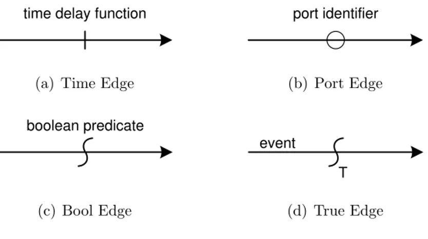
specifies a component’s state space through an augmented directed graph, where a state is depicted as a node and the possible state transitions are shown as directed edges among couples of node. Considering that a process should be suspended when it possesses the thread of control and then it may be reactivated [20, 95], all the states are possible process reactivation points (i.e., once a process has been reactivated, its thread of control starts again from the last visited state). Each AC has a set of local variables not visible by other components; these variables comprise a local simulation clock. Three attributes are associated to each directed edge: a condition, that defines when the arc is candidate to be traversed; a priority, that is used to decide which arc must be traversed when multiple edges are candidate for traversal at the same simulated time; and an event, which specifies the state transition that occurs during simulation whenever the arc is traversed.
time delay function
(a) Time Edge
port identifier (b) Port Edge boolean predicate (c) Bool Edge T event (d) True Edge
Figure 1.7: Edge notation in a CFG.
Edge conditions may be of the following types: time-delay, non-empty input port and boolean expression. Thus, we may refer respectively to TimeEdges, PortEdges and BoolEdges. A TimeEdge is equipped of a time delay function which returns a non-negative number representing the edge traversal time, i.e. how many simulated time from the current system clock the edge should be traversed. A PortEdge is an edge associated to an AC input port (many PortEdges can be associated to the same input port). For this edge type, the edge traversal is permitted when at least an un-received message is waiting into the message queue of the associated input port. A BoolEdge has a boolean expression which refer only to local variables. The
boolean expression must be evaluated to decide if the edge can be traversed. A sub-type of BoolEdge is called TrueEdge, that is a BoolEdge whose condition is defined to always evaluate to true. In Figure 1.7 is depicted the notation for all the edge types.
The event is an edge attribute that specifies a set of actions that must be executed when the edge is traversed. Allowed actions include changing in AC local variables, message sending to output ports, and only for PortEdges the message receiving from the associated input port. A null event occurs if no action must be performed during edge traversal (in this case the event is depicted with the function “e-null ”, but we prefer to omit it to ease the model readability).
Simulation execution is generally initialized by inserting messages into compo-nents input ports. Fritz and Sargent proposed a generic algorithm for model simula-tion, specifying how to identify the next traversed edge, when advancing simulation clock and how transfer the control between component states.
In a similar way as Schruben proposed for the EG models, whenever using ACs is necessary to design k instances of the same element (e.g. ports and edges), is possible to use multi-ports and multi-edges recurring to a vectorial notation [78, 37]. Multi-edges are depicted using a dashed line and the edge cardinality is shown in square brackets upon the edge.
In Figure 1.8 is shown an example of CFG for a SimpleServer AC as proposed by Sargent [78]. The behavior of this AC is described using the states “idle” and “busy”, designed respectively using the vertices “I” and “B”. Message arrival from the input port i1 represents the arrival of a job requiring processing. Whenever a message arrival takes place at the same time that the AC status is on the vertex B, then the message is queued in the message queue of the input port i1.
Modeling the behavior of ACs is straightforward in simple systems, but can become really complicated in large and complex systems. Therefore, Fritz and Sargent developed a hierarchical extension of CFG, called HCFG, which guarantees reusability and modularity. The behavior specification of an AC using HCFG is based on the idea that it should be decomposed in partial disjoint behaviors known as Macro Control States (MCSs). In that way, it is possible to depict the inner view of an AC by coupling MCSs (likewise for the inner view of a CC). A MCS is a
SimpleServer AC B I i1 e2 Functions: e1:
Receive message Job from i1; e2:
Send message Job to o1; t(s):
Generate service time using Service Distribution; e1 t(s) SimpleServer istanceName AC States: I = Idle B = Busy i1 (jobInput) o1 (jobOutput) CFG
Figure 1.8: The CFG for the AC SimpleServer (left side) and the outer view of the AC SimpleServer (right side).
SimpleServer AC
I
i1 e1
Functions: e1:
Send message Job to o1; t(s):
Generate service time using Service Distribution;
e1 t(s) SimpleServer istanceName AC State: I = Idle i1 (jobInput) o1 (jobOutput) HCFG Idle Busy MCS Idle MCS Busy State: B = Busy B Functions: e1:
Receive message Job from i1;
Figure 1.9: A HCFG for the AC SimpleServer.
CFG where nodes are states or MCSs, the input port and output port are explicitly depicted as pins. Thus, the simplest MCS is designed as a CFG. An MCS has no visibility of its outer view; then if a MCS or an AC encapsulates a MCS, its
local variables can not be accessed by the encapsulated MCS. The HCFG of the AC SimpleServer depicted in Figure 1.8 is given in Figure 1.9: this HCFG is composed of two MCSs, the MCS “Idle” and “Busy”. Comparing the inner view of the AC SimpleServer provided by the CFG in Figure 1.8 with the one described by the two MCSs of the HCFG in Figure 1.9, it is easy to recognize that the use of HCFG also improves the readability of the behaviour of an AC.
1.5
Holistic Discrete Event Simulation Models with
Process Interaction Modeling
Here we describe the MP called Holistic Modular Process (HMP) for developing simulation models originally proposed by Legato, Gull`ı and Trunfio [40]. A HMP model is a holistic MP for DES modeling based upon the PI worldview. Main concepts are presented in the following and its potentiality is illustrated by modeling a typical logistic process that arises in a maritime container terminal. Comparisons with the EG, PN and HCFG models are also provided.
1.5.1
Holistic Modular Process Simulation Models
The MP proposed in this paper is aimed to be flexible and expressive in the modeling of complex systems. It tries to achieve three primary objectives: model readability, reusability and personalization.
Model readability is a property which allows a model to be simple-to-read for a non-modeler. This property has a special importance when top managers are directly involved in scenario analysis: in our MP readability is achieved by describing the components’ behavior within a simulation model by a sort of flow-chart. As for re-usage property, our experience at the Gioia Tauro Container Terminal confirms the requirement that a specialized simulation tool has to be reused in some of its forms (model reuse, component reuse, function reuse and code scavenging [64]). Model reuse, under calibration and repeated tuning, occurs as soon as traffic conditions change over time. Furthermore, component and function reuse are both required to
give the operational manager the possibility of quickly implementing a first order model of some emerging situations, before the structured intervention of external expertise. According to our concept of holistic MP, we provide model reusability by means of hierarchical, modular model definition and redefinition of simulation parameters.
Model personalization is the base of an MP for the effective modeling of complex systems. It relies on the user-definition of process properties that allow describing uncommon situations, as it is the case when the modeler is asked to represent local, best practices in logistics organization and management.
An outline of the HMP simulation models follows now. An HMP model includes a set of model objects, or objects for short. For each model object an inner and outer view is defined. The outer view is depicted as a box equipped of input and output ports (see Figure 1.10). The inner view depicts a sequence of activities and events. The sequence is also called the model object process routine, or simply process.
TypeName InstanceName O I
Figure 1.10: The outer view of a model object in a HMP simulation model. In a similar way as described for HCFG models, relationships between model objects are depicted using directed edges (channels). Model objects are equipped with input and output ports (depicted as shown in Figure 1.10) that can, eventually, be renamed to improve model readability. Two model objects are linked by means of only one channel from an output port of the first object to an input port of the second object and vice versa, i.e. no more than two channels connect directly two model objects. Two model objects interact by message passing via channel, despite a channel has its own direction (the head of the edge is connected to an output port, while the tail to an input port). Multiple types of messages flow forward and backward along a channel, whilst entities (or jobs) of the simulation model can flow only through the proper channel direction.
T: ServiceStation I: aStation O I
(a) Outer view.
T: Queue I: Buffer O I T: Server I: Machine O I ModelType InstanceName O I (b) Inner view.
Figure 1.11: A sub-model depicting a service station, composed by a buffer and a server.
of model objects. Therefore, hierarchical modeling is pursued by coupling different processes and grouping the resulting net of model objects into a sub-model (which is depicted in a similar to a model object, as proposed in Figure 1.11). In this case, the model can be used to be coupled together with other model objects or sub-models. A requirement when constructing sub-models is that at least one input or output port must be defined and linked to the inner model-objects, otherwise, the depicted model is a super-model or final model. The inner view of a sub-model is just another HMP model where some channels link the inner part to the outer part of the model through its boundaries.
As stated above, the inner view of a model object is a process, or rather a sequence of activities and events that define the model object behavior. The process is represented as a particular hierarchical flow-chart, called Event-Activity Diagram (EAD), where activities and events are nodes and edges fix the logical and temporal sequence between nodes (other node types will be introduced in the following). A process can be constructed hierarchically by grouping events and activities to compose a process. Thus, a process is an EAD itself. By means of a sub-process we provide component reuse and model readability.
Similar to the conical methodology [55, 21], that is a framework for simulation model development, a model definition and specification using two main tools is provided.
The first tool is the model hierarchy structure (MHS). The MHS is a tree that provides a high-level model definition showing hierarchically the sub-models and
model objects that compose a simulation model (see Figure 1.12 for an example). Model 1 Model 2.1 Model 2.1.1 Object 2.1.1 Object 2.1.2 Object 1.1 Object 2.1.1.1 Object 1.2
Object 2.1.1.2 Object 2.1.1.3 Object 2.1.1.4
Figure 1.12: A Model Hierarchy Structure (MHS).
A more detailed model definition is obtained by a second tool, the EAD. An EAD provides the process definition. In fact, an EAD defines the structure of a process by means of a sort of flow-chart. Because of the possible use of sub-processes for the process definition, an EAD could be a hierarchical structure (composite nodes are expanded revealing a new EAD) and a hierarchical tree, similar to the MHS, may be used to explore the EAD structure.
1.5.2
Model Objects
Following the PI worldview, the first step consists in identifying all the model objects which are involved in system modeling and detect all common features. Then, class-dependent features are described for the few classes of model objects introduced in our MP. The objects are contextual, so it is necessary to specify the model in which they are defined. The model name parameter is used to declare which model an object belongs to. This parameter serves two reasons: first of all, the holistic approach says that such objects can only be used in some contexts; furthermore, the use of sub-models could cause a lot of confusion, especially if a sub-model is exploded (i.e. deleting model boundaries) and the same object is used in a model and in its sub-models. Objects of the same type are identified by the type name parameter. If the model name is a parameter that depends on the model, the type name is a non-changeable parameter. Each instance of a certain type of object is
also identified by the instance name parameter. The set composed by these three parameters univocally identifies a model object within an HMP simulation model.
There is at least another important parameter that allows managing heteroge-neous objects, known as category name. The use of the category name allows us to make associations between objects that are apparently disjoined. A possible use can be seen in the development of a simulation package, in the packages for statistical analysis and optimization of system performance measures. As a matter of fact, in this context generic rules and algorithms can be defined over a class of mixed objects - the benefits that can be derived by this approach has been investigated in a companion paper [48].
Model objects have a set of variables and data structures used to support the logical representation of the process behavior. These properties are not explicitly depicted and refer to the code implementation of each model object type. Model objects variables and data structures are accessed by a set of public functions which allow their manipulation. A function is called by message passing, or rather sending an explicit message to call a specific model object function.
Model objects are illustrated in detail in the following.
There are two basic classes of objects: resources and resource managers. As stated above, entities of the simulation model are depicted as messages that are able to envelop properties, data structures and other entities (e.g., a ship that carries thousands of containers loaded in different holds).
Resources are active or passive depending on their role in the simulation model. Passive resources are not depicted explicitly and are not able to execute action/events or process entities. Nevertheless, a passive resource is able to execute incoming re-quests and actions of other model objects (as declared above, a passive resource shows a set of public functions that can be used to manipulate the resource). Pas-sive resources are generally managed by an active resource or a resource manager. Whenever a passive resource is managed by a resource manager, active resources linked to the resource manager are able to overwork it only under the conditions specified by the resource manager. A passive resource must be managed by a re-source manager if more than one rere-source may request it for use during a simulation (e.g., items storage into a shelf using forklifts). An active resource can possess
passive resources and it can offer a service to one or more entities per time. It can also make queries to other objects to which it is linked by message passing via input/output ports. The behavior of an active resource is described using an EAD. By means of resources one can only represent just a system governed by a few simple rules. As matter of fact, the need of modeling complex systems in a holistic approach leads us to introduce the resource managers. A resource manager is a high-level object, which is able to interact with a set of model objects (also het-erogeneous). Resource managers can take decisions (e.g., solve a scheduling or an assignment problem, negotiating the use of a sub-system, etc.) by applying rules and policies and making queries to other model objects. They have free access to modify the behaviour of all the resources in their own model to which they are linked. In a holistic approach, as demonstrated by Pidd and Castro [67], the use of that kind of model objects avoids the explosion of object links and therefore it represents a more easy-to-use modeling tool.
1.5.3
Processes and Event-Activity Diagrams
The role of a process in model object specification is analyzed here and process representation is shown. The interaction of processes during the simulation is briefly described.
According to the definition of process given in the PI worldview overview, a process is a series of temporally related events and activities. Usually flow-charts may be used to represent processes. In our flow-charting methodology, called Event-Activity Diagram (EAD), events and activities are nodes, while directed edges define one or more paths that can be covered by a process. Other useful elements compose a process, namely the logical nodes.
Activities and events are not intended to perform actions, but to show to non-modelers, in a friendly-way, how a process can work. The role of executing requests, performing actions and introducing time delays between activities and/or events is assigned to directed edges. Therefore, the use of a flow-charting graphical method-ology to depict a process allows us to achieve at a good extent the readability ob-jective. Bearing in mind the list of the process components, let us start an in-depth
discussion about these components.
In our MP, activities are classified focusing on the simulation duration of the activity; hence activities are partitioned in timed and instantaneous. The first type of activities are those able to start operations at a simulated time instant and finish operations in a future simulated time instant. For instance, timed activities are those that perform operations characterized by a variable simulated time length, e.g. waiting or servicing activities. The second type refers to activities that start and end operations at the same simulated time instant, e.g. activities representing a choice or check by a resource or resource manager. Nevertheless, also timed activities can starts and ends operations at the same simulated time instant.
A process needs the specification of an initial activity that is enabled, or rather the activity that possesses the process checkpoint (more details about checkpoints are provided in the following). The initial activity is the activity from which the process starts when it becomes active (initial process state). In an EAD one or more activities per time can be enabled, i.e. when the process flow has been forked in different logical paths. The set of currently enabled activities is called the process state.
An event is a fact that forces one out of a set of possible changes of the current state. It may precede or follow an activity, thus representing something that is just happened or that is going to happen. If an event precedes an activity, then it is processed at the same simulated time of the activity start; if an event follows an activity, then it is processed at the same simulated time of the activity end.
As stated before, EADs have a hierarchical process structure. In fact, nodes are activities and events and even sub-processes. A sub-process is itself an EAD, therefore it can be zoomed revealing the included flow-chart. The EAD of a process can refer to input and output ports of the including process, i.e. a sub-process is only a convenient arrangement for grouping an EAD sub-net and depicting it as a single node (this solution aims to improve model readability).
The different shapes for the main nodes of an EAD are depicted in Figure 1.13. The core of the process behavior is designed adding directed edges. Edges are used i) for message passing and the evaluation of conditions through functions call, and ii) for the introduction of timing into process activity flows. We classified edges
Timed Activity
Event
Istantaneous Activity
Sub-Process
Figure 1.13: Nodes of an EAD.
in four types: null edges (or true edges), inner edges, incoming edges, outgoing edges. A null edge can be used only to connect events to activities or activities to activities. An inner edge connects an activity to another activity or to an event. These edges are depicted as arcs (see Figure ??). Incoming edges are used to depict incoming messages from an input/output port, while outgoing edges depict outgoing messages to an input/output port. Incoming edges connect only activities to activities or activities to events, while outgoing edges also link events to activities. Edges may not have any node linked to the head, thus they work as a termination arc (i.e, the process becomes definitely terminated when one of these nodes is traversed).
Requests Conditioning Requests Actions
Inner Edge
T()
Incoming Edge
Actions
Port>Request Conditioning Requests
Outgoing Edge
Actions
Port<Request Conditioning Requests
Null Edge
T()
Figure 1.14: Edges of an EAD.
Edges produce a transition from the current enabled node (connected to the edge tail) to the future enabled node (that is linked to the edge head). To avoid deadlock, edge tail and head must be different nodes. While the transition rule for a null edge is always true, for the other edge types the edge traversal is allowed only if certain conditions are met. To understand the nature of these conditions, we introduce the
following edge functions: a Timer and a Request.
A Timer is a time function that generates a delay time using a probability dis-tribution function (e.g., exponential) and the appropriate set of parameters. Only inner and outgoing edges may have a Timer. Whenever an inner/outgoing edge is selected by an activity to be eventually traversed, the Timer generates the simulated delay time and an “alarm” is scheduled to warn the edge after the delay time. When an edge has been warned, it is allowed to enable its head node (i.e., the process state has been changed), or rather it is traversed.
The transition rule of an edge is composed by a set of Requests. A Request is a (public or private) function of a process that can be called to check conditions, to set up model objects and entities parameters and (in case) exchange entities among model objects. If the conditions are met, the function returns true; false, otherwise. A set of primary Requests can be used on the same edge by the formulation of a logical expression using boolean operators (and, or, xor ) and negation (not), that we call the primary rule; moreover, the verification of the primary rule may depend on a set of conditioning Requests, or what we call the conditioning rule. Both conditioning and primary rules compose the transition rule in the following way: “primary rule | conditioning rule”. Only if the conditioning rule is evaluated as true, then the primary rule is evaluated.
All the edge types (excepted null edges) may have a transition rule. A con-siderable difference exists between inner and incoming/outgoing edges. In fact, by using incoming/outgoing edges, a process can: i) make a call to a public function of an external process (receiver process) linked to an input or output port; ii) receive a call to its own public functions by an outer process (sender process) linked to an input or output port. In this way we enable communication among processes (e.g., exchanging entities and assigning work). In particular, the primary rule of an incoming (outgoing) edge must only include the call of a Request by (of) another process linked to an input/output port. The symbolism used to call a Request of an outer object is “PortName<Request”, while to depict the call of a Request by an outer object “PortName>Request” is used. For incoming/outgoing edges, the conditioning rule may also include calls to outer functions.
least an incoming edge starting from the current node of the receiver has the called Request as primary rule, then the call to the Request function may return true; otherwise, false is automatically returned (i.e. the call is not accepted). Indeed, incoming edges work as triggers for processes that are waiting for an external input. With the exception of null edges, which are always traversed, if an inner edge (or an outgoing edge) is selected to be traversed by the current node, then it is traversed once the traversal rule is true.
Timers and Requests are the condition functions that may be involved to cause an edge traversal. Nonetheless, inner and outgoing edges may have both a Timer and Request function. In this case, the execution priority states that the Timer must be executed before a Request, i.e. the transition rule is verified when the edge has been warned.
All the edges may also have a list of Action functions. An Action is a function that performs such operation, e.g. changing the parameters of the process or of an owned entity. If a Timer and/or a transition rule have been defined for the same edge, the Action must always be executed at last, i.e. after the edge has been warned and if true has been returned by the transition rule.
Each Request and Action can explicitly receive a set of parameters; therefore, the behavior of a Request/Action may change in function of the received parameters.
To improve MP scaling and model object reusability, as proposed in [78], each process may use multiports. A multiport is an indexed set of k ports named port-name[1],. . . , portname[k]. A multiport is explicitly depicted as different ports in the external view of a model object; in the inner view, multiport may be used either in an explicit or implicit way by incoming/outgoing edges. For instance, an explicit use of a multiport may occur when the process needs to call a Request function of an external process linked to the port “portname[i] ” (where the suffix [i] stands for the index of a port that is included in the multiport portname[1,. . . ,k] ), then the name of the port is explicitly depicted in the transition rule of the function as follows: “portname[i]<Request”. Another example is introduced to show the implicit use of a multiport. If the process needs to call the same Request function of the external processes linked to the multiport, the following notation must be used in the tran-sition rule of the outgoing edge: “portname[i:1,. . . ,k]<Request”. In this way, for
each portname[i], where index i varies between 1 and k, the edge must check the associated transition rule and the edge is traversed whenever at least one transition rule is true. The implicit use of a multiport allows our MP to be compact and to easily implement the behavior of dynamic processes. Moreover, by using implicitly a multiport, it is possible to specify a sub-set of port indexes that i) must be called through an outgoing edge or ii) allow an external process to call an inner Request through an incoming edge. The sub-set of port indexes can also be a list name generated at runtime using an Action function.
Our MP allows defining a process behavior via EAD using activities, events, sub-processes and directed edges. Another type of nodes, called logical nodes, has been defined in order to support the definition of process paths. These nodes are: i) boolean fork ; ii) split; iii) and ; iv) or ; v) unconditional flow (Figure 1.15). A logical node may be used to represent alternative paths to be chosen under specified conditions.
Boolean Fork Split
And Or
Unconditioned Flow
Figure 1.15: Logical nodes of an EAD.
A boolean fork can be connected to the head of a conditional edge, or rather those edges that have a transition rule. Using this node, if the transition rule is true, then the edge is traversed and the process control flows through an edge starting by the boolean fork node; otherwise, the edge is also traversed, but the process control flows through a special edge, depicted with a dashed line, which starts by the boolean fork node. Therefore, using the boolean fork node after a conditional edge, the edge is always traversed. The outgoing edges from a boolean fork node are of the null or inner type. In case inner edges are used, another boolean fork must
be used for each inner edge to catch the result of the transition rule.
The unconditional flow node acts in a similar way of a boolean fork, but whatever be (true or false) the transition rule of the incoming edge, only one edge must leave this node.
The remaining logical nodes may be connected to the head of any edge type. Once the edge is traversed, the process control passes at the logical node. A split node is used to separate the process path in two or more alternative paths. When the process path is separated in more paths, to recombine two or more paths, an and/or node is required. The and node, becomes enabled at the time all the edges incoming to the node have been traversed. The or node become enabled at the time at least one of the edges incoming to the node has been traversed.
The and, or and split nodes can be part of the process state. Typically the process state has only one active activity per process state. However, once the process flow is separated by using a split, many activities and the split/and/or nodes may be enabled, thus they may be part of the process state.
Some explanations are required about the use of sub-processes as nodes of an EAD. As they are EAD nodes, edges that start and arrive to these nodes are of the types defined in the previous. The only restriction is for edges that start by a sub-process node. If an edge that starts from a sub-process node is not a null edge type, a boolean fork must catch the edge transition results (otherwise the process checkpoint may stay on an edge included in the sub-process). The inner view of a sub-process is a particular EAD which consists of at the most one edge that links the outer view to an inner node (or rather from the inner boundary to a node) and/or at the most one edge that links an inner node to the outer view (or rather from a node to the inner boundary). Also if the edge that starts from the sub-process inner boundary to a sub-process node is not of null edge type, a boolean fork must catch the edge transition results (otherwise the process checkpoint may stay on an edge included in the sub-process). An example about a finite queue is shown in Figure 1.16.
Processes are usually executed during more simulation time periods. For this reason the nodes of a process can be visited during different time periods. To track this possibility, we adopt the process checkpoint. A process checkpoint is a property