Antireflection coatings from analogy between electron scattering
and spin precession
D. W. L. Sprunga) and Gregory V. Morozov
Department of Physics and Astronomy, McMaster University, Hamilton, Ontario L8S 4M1 Canada J. Martorell
Departament d’Estructura i Constituents de la Materia, Facultat Fı´sica, University of Barcelona, Barcelona 08028, Spain
共Received 24 September 2002; accepted 20 January 2003兲
We use the analogy between scattering of a wave from a potential, and the precession of a spin-half particle in a magnetic field, to gain insight into the design of an antireflection coating for electrons in a semiconductor superlattice. It is shown that the classic recipes derived for optics are generally not applicable due to the different dispersion law for electrons. Using the stability conditions we show that a Poisson distribution of impedance steps is a better approximation than is a Gaussian distribution. Examples are given of filters with average transmissivity exceeding 95% over an allowed band. © 2003 American Institute of Physics. 关DOI: 10.1063/1.1559942兴
I. INTRODUCTION
Antireflection coatings共ARC兲 are of great importance in many areas. In optics the aim is to maximize the transmis-sion of visible light through lenses by applying coatings with suitable indices of refraction on both surfaces. For micro-wave transmission, the analogous problem is to minimize reflection at a junction between two sections of waveguide, by means of an impedance transformer consisting of sections of varying cross-section. Solutions for these problems were worked out in the 1950’s and can be found in many books and reviews, of which we cite some representative examples.1– 6
Recently Gornik’s group in Vienna7,8 have studied the analogous problem of constructing an energy bandpass filter for electrons in a semiconductor heterostructure. In a first paper they demonstrated a single-cell ARC, which raised the transmissivity through a superlattice to about 80% across the lowest-allowed band. In further work they proposed a double-cell device with even better properties. We have de-rived exact criteria for optimizing the properties of a single-cell ARC.9
The problem of constructing a passband filter for elec-trons has been discussed by several groups. Gaylord and collaborators10,11very early wrote a series of papers propos-ing to take over the well-established solutions from optics and microwaves. Chang and Kuo12 translated the Gaylord approach into the language of impedance transformers. Tung and Lee13and later Gomez et al.14considered a rather differ-ent filter based on a Gaussian distribution of barrier strengths. Yang and Li15 extended this approach by using a variety of different distributions, but with no underlying theory as to why these might or might not work. In other words, previous approaches have either relied on the similar-ity to optical and microwave ARCs, assuming that this
well-developed theory would apply to electrons, or else they sim-ply guessed at how to proceed.
The aim of the present article is threefold. First of all, we draw attention to an interesting analogy between共i兲 a particle scattering in a one-dimensional potential and 共ii兲 a spin-half system precessing in a magnetic field. Second, we use this analogy to give a simple and intuitive explanation of how an impedance transformer, and consequently a bandpass filter, works. While such a picture does not entirely dispense with the ingenious calculations underlying the classical recipes for ARC cells and impedance transformers, it certainly provides insight to the crucial issues involved. In particular, it leads to the concept of stability conditions and their role in defining the parameters of an N-cell ARC.
Our third contribution is to identify the most important difference between bandpass filters for electrons and their counterparts in optics. This leads us to propose a simple model, called the linear model, which is similar to the true situation for electrons in semiconductor superlattices. We solve this model analytically, and show that the resulting filter is very different from the well-known Butterworth or binomial filter of optics or microwave engineering. As a practical application, our method is applied to the device of Pacher et al. and Coquelin et al.7,8 We find that their trans-missivity could be significantly improved by following our method.
II. TRANSFER MATRIX
In the single-band envelope function approximation, the electron wave function satisfies the Schro¨dinger equation in a real potential and with an energy- and position-dependent 共real兲 effective mass16m*(E,x)
⌿共x,t兲⫽e⫺iEt/ប共x兲
d2共x兲 dx2 ⫹
2mm*
ប2 关E⫺V共x兲兴共x兲⫽0
a兲Electronic mail: [email protected]
4395
k2共x兲⫽2m
ប2 m*共E,x兲关E⫺V共x兲兴. 共1兲
The time-reversed spatial wave function is*(x). Con-sider a potential cell, placed ⫺d⬍x⬍d. Outside the cell, assuming zero potential, k becomes constant and we may write the wave function in the form
共x兲⫽ae⫹ik(x⫹d)⫹be⫺ik(x⫹d), x⭐⫺d,
共2兲 ⫽a
⬘
e⫹ik(x⫺d)⫹b⬘
e⫺ik(x⫺d), x⭓⫹d.The amplitudes on opposite sides of a cell are related by
冉
a b冊
⫽冉
M11 M12 M21 M22冊
冉
a⬘
b⬘
冊
, 共3兲which defines our transfer matrix M . It has the properties det M⫽1, and through TrM⫽2 cos, defines the Bloch phase associated with a periodic array of identical cells.
For a scattering problem with incident wave from the left, a⫽1, b⫽rL⫽r; a
⬘
⫽tL⫽t, b⬘
⫽0, one easily sees that the first column of M is given byM11⫽
1
t, M21⫽ r
t. 共4兲
The second column of M is determined by conservation of flux, and by the corresponding equation for incident waves from the right, with amplitudes denoted rR⫽r
⬘
,tR ⫽t⬘
. For a general potential, one can show that t⬘
⫽t, and r⬘
/t⬘
⫽⫺r*/t*. The result is M⫽冉
1 t ⫺ r⬘
t⬘
r t 1 t*冊
⫽冉
1 t r* t* r t 1 t*冊
共5兲without assuming parity invariance. Time reversal symmetry alone makes M12⫽M21* and M11⫽M22*.
For a potential with reflection symmetry the additional property rR⫽rLholds, which makes M12⫽⫺M21⫽M21* pure
imaginary. Following Kard,3 for a symmetric cell we can introduce a parametrization of M , valid in an allowed band M11⫽cos⫺i sincosh⫽M22*,
M21⫽⫺i sinsinh⫽M12*, where
cos⫽1
2Tr M⫽Re M11, and tanh⫽Im M21/Im M11. 共6兲 This form respects the relation 1⭐1/兩t兩2⫽1⫹sin2sinh2 as well as det M⫽1, but applies only in an allowed miniband where the Bloch phaseis real.17We callthe impedance parameter, because in the case of a square well, e is the impedance, the ratio of velocity outside to inside the well.12 For an arbitrary cell, a different phase  occurs on the off-diagonal elements
M21⫽⫺eisinsinh⫽M12*. 共7兲
The symmetric cell corresponds to the special case  ⫽⫹/2. For the moment we confine our attention to sym-metric cells for which we write
M⫽cos
冉
1 0
0 1
冊
⫺i sin冉
cosh ⫺sinh sinh ⫺cosh
冊
⫽cosI⫺i sinU共2兲,with U共2兲⫽coshz⫺i sinhy⫽•nជ, 共8兲 where nជ is a 共complex兲 unit vector in the YZ plane. The meaning of this becomes evident if we write ⫽i, giving
M⫽e⫺in⫽R n共2兲,
where n⫽•n⫽cos z⫹sin y. 共9兲 We recognize Rn as the operator which rotates a spin-1/2 system by angle 2 around the axis n,18 which in this in-stance lies in the Y Z plane. For asymmetric cells, the axis of rotation has azimuthal angle. The axis of rotation is imagi-nary, but this does not invalidate the analogy.
Now consider an array of cells which need not be iden-tical. The transfer matrix for the pth cell is of the same form as Eq.共8兲, with parameters p andp⫽ip. It can be fac-torized as follows:
Mp⫽e⫹i(p/2)xe⫺ipze⫺i(p/2)x
⬅Y共p兲P共p兲Y共⫺p兲. 共10兲
Y () is associated with a step-up in impedance from zero to
. The factors can be interpreted as follows. The top line is a rotation operator acting to the right on a ket. The spin-half system is rotated around OX by angle p, so an axis in-clined initially at angle p, lines up along OZ. Then the system is rotated by angleparound OZ, and finally rotation around OX by angle ⫺p restores the axis to its initial po-sition. The net effect is a rotation of the whole system by angle p around the axis of rotation oriented at polar angle
p. In the second line, a system consisting of left/right mov-ing waves is acted on by a transfer matrix. The first factor lowers the impedance byp; then it propagates freely accu-mulating phase ⫿p on the upper/lower components, and finally the impedance is restored to its original value. The net effect is the same as propagating at an average impedancep and accumulating the same phase.
In this analogy, a wave traveling to the right, outside the array, corresponds to a spin-up共along OZ兲 state, and a wave traveling to the left, to a spin-down state. When a right-moving state encounters a potential, it is partly transmitted and partly reflected. Analogously a spin-up state placed in a magnetic field oriented at polar angle will precess around the field direction, thereby acquiring some spin-down 共re-flected wave兲 component. For a symmetric potential cell, the magnetic-field direction lies in the Y Z plane. For a general cell, the polar angle is the same, but the azimuthal angle is: The asymmetric system differs only by a rotation around OZ.
This analogy is very helpful in seeing how a system will respond to a sequence of potential cells. For identical cells
p⫽;p⫽, the rotations are all about the same axis. The spin precesses on a cone whose polar angle is ; the cone intersects the sphere in a circle. Viewed from above the unit sphere, the spin moves on a circle centered at. If there are N such cells, the total angle of rotation will be 2N. The condition for perfect transmission is that the spin state be returned to lie along OZ; this requires 2N⫽2m where m is an integer. Within an allowed band, the Bloch phase in-creases by, so the possible values are m⫽1,2,...,N⫺1. An array of N identical cells will show N⫺1 narrow resonances in each allowed band.19 They are narrow, for when the en-ergy is varied slightly, changing →⫺, the total phase changes by 2N, which quickly moves off the resonance condition. This situation is illustrated in Fig. 1 for an array of seven cells, and for m⫽1; the phase angle is off resonance by 1%. One is looking down on the surface of the sphere from a point above the center of the circle. The radial lines mark off sectors of angular width 2⬇2/7.
If the cells are not identical, but the impedance param-eters p are close, then the sequence of rotations will be on arcs of circles whose centers jump about. So long as these jumps are small compared to the radii of the circles, the total angle of rotation will be just twice the sum of the anglesp. The behavior of the array will then be similar to a strictly periodic array. It will still wind N times around a closed path, coming more or less close to the origin共at OZ兲 once on each traversal. We will have similar behavior to the case of iden-tical cells, but with the sum of the p playing the role of N. This is the ‘‘mean phase lemma.’’
Conversely, if thepare increasing rapidly, so the center of each rotation lies outside the circle of the previous one, then the path followed on the surface of the unit sphere will not wind more than once around the circumference. We will see that this topologically very different behavior is charac-teristic of impedance transformers and filters.
III. QUARTER-WAVE IMPEDANCE TRANSFORMER In this section we will show that the criteria for quarter-wave filters can be easily understood from our spin analogy. Further we will show that the classic recipes do not apply to
the semiconductor case unless significant modifications are made. These lead to the conclusion that a Poisson distribu-tion of the impedance steps between cells is more appropri-ate than is a Gaussian recipe.
For an electron in the conduction band, a layered hetero-structure acts as a series of nonoverlapping potential cells. A cell can contain any number of homogeneous layers, or may even be continuously graded. No matter how complicated the potential共or the effective mass兲 may be, the scattering prop-erties of a single cell are described by just two 共or three兲 energy-dependent parameters,共and兲.
As discussed in Ref. 9, the first step in designing an energy bandpass filter is to find a cell with an allowed mini-band covering the desired energy range. If it is the lowest-allowed band, then cos(Eᐉ)⫽1 and cos(Eu)⫽⫺1 at the lower- and upper-band edges. By placing a number K of such cells together, a well-defined miniband will be obtained with essentially zero transmission outside the allowed band. If the cell is symmetric, any number of them will also be reflection symmetric, and the transfer matrix MXK for this array will be described by just two parameters,X andX. An ARC consists of an additional potentialvA(x) placed on one side of X and its reflection vA(x) on the other side. The corresponding transfer matrices will be denoted A and A. According to the spin analogy, A rotates the spin by angle 2A about an axis specified by its impedance param-eters A and A. For simplicity consider the case where both X and A are symmetric cells. Then the axes of rotation both lie in the Y Z plane. At an arbitrary energy in the al-lowed band, if A rotates the initial spin-up state by angle, it will be converted to a state whose spin is oriented along another radius in the Y Z plane. By choosingA⫽X/2, the new orientation of the spin state will coincide with the direc-tionX. Passing through the potential cells X alters the spin state only by a phase factor ⫿X, because the new state is an eigenstate of spin along this direction.
Rotation by angle means that A⫽/2, so that the ARC cellvA must be a Bragg reflector at the desired energy. This is the solution obtained in Ref. 9. The downstream ARC cell A then rotates the spin state back to lie along OZ, representing a wave moving purely to the right, and giving perfect transmission. The path followed by the pseudospin state is illustrated in Fig. 2共a兲. It does not matter how many cells of type X there are, because once the state is aligned along the direction X it is in a spin eigenstate along that direction, and precession gives just an overall phase, which does not alter the probability of being in a spin-up or -down state along OZ. Such a state is a scattering eigenstate for the potential vX.
An ARC may consist of more than one cell, for example two as illustrated in Fig. 2共b兲, or three in Fig. 2共c兲. In the general case we will number the cells 1,2,...,N on the left, with the reflected ordering on the right. Let MX be the trans-fer matrix for the central cells, 共the original system兲. Then, using the representation of Eq.共10兲, the total transfer matrix can be written in two equivalent forms
MT⫽AMXA⫺1*⫽AY共X兲P共X兲Y共⫺X兲A⫺1*
⬅M P共X兲M⫺1*. 共11兲
FIG. 1. Pseudospin path viewed from above for a periodic system with
In the first form, A represents an impedance transformer, which takes the incident plane wave and prepares it to propa-gate through the central cells, described by MX.
In the second form, A is combined with a step-up opera-tor Y (X) which undoes this, rotating the state back to the OZ axis, so that the propagator P(X) need only supply the phase factors⫿X as the wave propagates through the cen-tral cells. In detail, M consists of
M⫽M1M2¯MNY共X兲. 共12兲
According to the spin picture, when M acts on a state 兩⫹,Z
典
which is ‘‘spin-up’’ along OZ, it has to leave it in the same condition. This requires that the element M21⫽0. Thereflected operator M⫺1* performs the inverse rotations, re-storing the state to be spin-up along OZ. It is sufficient to construct M in order to make a passband filter. Incidentally, this proves that the design of a passband filter, at the design energy, does not involve the Bloch phase X of the central cells. While it may appear complicated to combine Y along with A, it is actually a big simplification, because each of the
transfer matrices Mk needs to be considered only once, not twice as would be the case if we worked with MT.
In the classic designs, each cell of a multicell ARC is reflection symmetric, so M and M⫺1* differ only in the reverse ordering of the cells, and replacement of the step-up impedance factor Y (X) by a step-down, Y (⫺X). In this case, the simplest solution is to make each cell into a Bragg reflector at the design energy, withp⫽/2. Such a solution was illustrated in Fig. 2共b兲, for N⫽2 cells. The question arises, what possible advantage can come from using two cells as opposed to a single cell? The answer is found by supposing that the energy is varied by a small amount, so that p→/2⫺p. Then on the first rotation, the spin does not quite reach the axis. In the small angle approximation, the second rotation has a head start by 21, and it will land
within 2(2⫺1) of the pointX. If the phases p are in fact equal, then the two deviations cancel out, and the N ⫽2 filter will have first-order stability. Since the single-cell filter has no such compensation available, it will go off reso-nance as soon as the energy varies from the design energy. The two-cell filter goes off resonance only when the squares p
2
become significant.
The situation of equal Bloch phases in every cell gener-ally applies in optics or microwaves, because 共for normal incidence兲 the phase accumulated in passing through a cell is just p⫽k0npap, the product of wave number in vacuum, the index of refraction, and the cell thickness.共Usually a cell is a single homogeneous layer in optics.兲 If the p are ar-ranged to be equal at the common Bragg point, then they will remain equal so long as the index of refraction is constant. This is not the case however in semiconductors because the wave-number k(x) is the square root of an energy difference, as in Eq. 共1兲.
For N⫽3 cells the classic Butterworth filter design has
1⫽1/8X, 2⫽1/2X, and 3⫽7/8X. In units of X, the rotations of the spin analogy have radii 1/8, 1/4, and 1/8, as illustrated in Fig. 2共c兲. It is not hard to see that this model also shows linear stability as the energy varies from the multi-Bragg point, with a deviation in angle of twice 1
⫺22⫹3 which vanishes when thep are all equal. More-over, this design also exhibits quadratic stability, defined as second order in the p. In other words, the zero of the re-flection amplitude at the design energy will be a second-order zero, leading to a flatter maximum in transmission. Comparing the three panels of Fig. 2, one sees that the Bloch phases k can be further off the Bragg point when N is larger, and the device can still give very good transparency. IV. ANALYTICAL DEVELOPMENT
At this point it is useful to derive and extend the above results analytically. From Eq. 共10兲, for each symmetric cell included in the ARC transfer matrix M , we can write
Mp⫽⫺i sinp关U共2p兲⫹i cotpI兴. 共13兲 For brevity, we will write Up for U(2p). At the design energy, every p⫽/2, and M reduces to a product of U-matrices. This product is easily reduced because the mul-tiplication table for the U and Y matrices is very simple:
FIG. 2. Pseudospin paths for binomial ARCs. Thekare off the Bragg point
U共兲⫽
冉
cosh/2 ⫺sinh/2 sinh/2 ⫺cosh/2
冊
, Y共兲⫽冉
cosh/2 sinh/2 sinh/2 cosh/2
冊
⫽e(/2)x,
UaUb⫽Y共a⫺b兲, UaYb⫽U共a⫺b兲, 共14兲 YaUb⫽U共a⫹b兲, YaYb⫽Y共a⫹b兲.
Like matrices give a Y ; unlike give a U. If a Y is to the left we get the sum of arguments, and if a U, the difference. Therefore at the Bragg point we can reduce the product as follows: 共i兲NM⫽
兿
p⫽1 N U共2p兲Y共X兲 ⫽Y共21⫺22兲兿
p⫽3 N U共2p兲Y共X兲 ⫽U共21⫺22⫹23兲兿
p⫽4 N U共2p兲Y共X兲¯ . 共15兲 If N is even we arrive at the penultimate step with a Y whose argument is an alternating sum of’s, ending with ⫺2N. The last multiplication uses the rule for Y⫻Y, which addsX. When N is odd, we end up with a U, whose argument ends with ⫹2N, and the U⫻Y product gives a Y whose argument共denoted⌺) ends with 2N⫺X. In either case, the matrix element is M21⫽sinh⌺, and the condition for zero reflection is that⌺⫽0. Explicitly,
⌺⫽
兺
p⫽1 N
共⫺兲p⫹12
p⫹共⫺兲NX. 共16兲
All the equations we will deal with are simpler when written in terms of the steps in,共including0⫽0), which
we define as ⌬p⫽p⫹1⫺p. Then we can write
⌺⫽
兺
p⫽0 N 共⫺兲p⌬ p⫽0 while X⫽兺
p⫽0 N ⌬p. 共17兲For a single-cell ARC, N⫽1, the solution is ⌬1⫽⌬0
⫽X/2, so 1⫽X/2. In terms of indices of refraction, for the optical case this is the well-known solution n1⫽
冑
nXn0.For more than one cell these two conditions are not suf-ficient to select a unique solution. A solution can be written down by considering the function
FN共x兲⫽
兺
p⫽0 N xp⌬p with FN共1兲⫽X; FN共⫺1兲⫽⌺⫽0. 共18兲The Butterworth6or binomial solution makes FN(x) propor-tional to (1⫹x)N, by setting
⌬p⫽
X
2N NCp⫽⌬N⫺p. 共19兲
So it is the steps, not the impedances themselves, which are the simple quantities. The N⫽2 and 3 filters drawn earlier are of this type. The solution is plausible if you interpret x ⫽e2ias being the same for every cell, and taking the value
⫺1 at the multi-Bragg point. Then the matrix element M21
will have an Nth order zero there.
Even for moderately large N, the limit of the binomial distribution is a Gaussian. With the steps ⌬p obeying a Gaussian law, thep will be distributed like the error func-tion. This may be the basis for the folklore that a Gaussian distribution of barrier heights should be associated with ARC cells.
V. STABILITY CONDITIONS
For small deviations from the multi-Bragg point, we write p⫽/2⫺p, and in Eq. 共13兲, the cotp becomes tanp⬅tp for short. We treat the tp as small quantities, and derive stability conditions which involve m of them at a time.
Using the representation Eq.共13兲 in the product of Eq. 共12兲, and grouping terms with the same number of tp, the general form of the transfer matrix becomes
M⫽
兿
p⫽1 N 共⫺i sinp兲冋
兿
p⫽i N Up⫹i兺
k⫽1 N tk兿
p⫽k Up ⫺兺
k⬍m tktm兿
p⫽k,m Up⫺i兺
k⬍m⬍r tktmtr兿
p⫽k,m,r Up ⫹¯册
Y共X兲. 共20兲Using the multiplication table for the matrices U it is straightforward to write down the terms of any order. The leading term involves no tk. Then there are sets of terms which involve 1,2,3,..., of the tk. The first N⫺1 of these sets give stability conditions which must be imposed to make the resulting transmission amplitude as flat as possible in the region around the multi-Bragg point. The last term involves the product of all the tk and is simply
M⫽Y共X兲
兿
p⫽1N
cosp. 共21兲
This is what remains when all the stability conditions have been satisfied, and is the generalization of the Butterworth filter for unequal phasesp.
The linear stability terms are obtained by including one of the tk⫽tan kin place of the factor Ukin the product Eq. 共12兲. The typical contribution is
␦(1)M⬃U
where Up⫽U(2p). Because Uk is missing from the prod-uct, the result of these multiplications is to arrive at either a U or Y matrix whose argument differs from ⌺ in two re-spects: 共i兲 the argument 2k is missing and 共ii兲 the terms following k⫺1 have the wrong sign as compared to ⌺. The typical case is
21⫺22⫹¯⫹2k⫺1⫺2k⫹1¯
⫽⫺0⫹21⫺¯⫹2k⫺1⫺k⫹k⫺2k⫹1¯ ⫽⌬0⫺⌬1⫹¯⫺⌬k⫺1⫺⌬k⫹⌬k⫹1⫹¯
which is to be compared with ⌺:
0⫽⌬0⫺⌬1⫹¯⫺⌬k⫺1⫹⌬k⫺⌬k⫹1⫹¯ . 共23兲 The contribution of this term to M21 involves a factor tk times the sinh of this argument. Again the aim is to make the 2,1 matrix element vanish, which means that the sum of all these contributions must be zero. We can simplify the argu-ment of the sinh by adding to it ⌺ which is already zero, 共the last line above兲. Then the terms following ⌬k⫺1cancel out. As a result we can write the linear stability condition as follows: ␦(1)M⫽
兺
k⫽1 N tksinh冋
兺
p⫽0 k⫺1 共⫺兲p⌬ p册
⫽0 ⫽t1sinh⌬0⫹t2sinh共⌬0⫺⌬1兲 ⫹t3sinh共⌬0⫺⌬1⫹⌬2兲⫹¯ . 共24兲In the small angle approximation for the hyperbolic func-tions, this expression agrees with the linear stability condi-tion for the filters drawn in Fig. 2.
The quadratic stability condition arises from terms where two of the matrices UkUmare replaced by tk,tm fac-tors. For the three-cell case N⫽3, one has
t1t2U3Y共X兲⫹t1t3U2Y共X兲⫹t2t3U1Y共X兲 ⫽t1t2sinh共3⫺X/2兲⫹t1t3sinh共2⫺X/2兲
⫹t2t3sinh共1⫺X/2兲
⫽t1t2sinh共1⫺2兲⫹t1t3sinh共1⫺22⫹3兲
⫹t2t3sinh共3⫺2兲
⫽t1t2sinh共⫺⌬1兲⫹t1t3sinh共⌬2⫺⌬1兲⫹t2t3sinh共⌬2兲.
共25兲
It is easily seen that this vanishes for the binomial filter, providing that the tk are all equal. But for semiconductors where they are unequal, it is a new condition to be imposed on the ⌬k.
The general mth-order stability condition is worked out in Appendix A. It takes into account all terms where m of the tkare involved, for m⫽1,2, . . . ,(N⫺1).
VI. PRACTICAL APPLICATION OF STABILITY CONDITIONS
For an N-cell impedance transformer, Eq.共20兲 expresses M as a sum of 2Nterms, which fall into N⫹1 classes labeled by the number m of tkoccurring in the terms of class m. The matrix element M21 must be zero for perfect transmission
into the central cells X.
The vanishing of the m⫽0 term is expressed by ⌺ ⫽0 in Eq. 共17兲. It involves just the alternating sum of the steps ⌬k, k⫽0 ¯N. The linear, quadratic, and higher sta-bility conditions involve products of the tktimes hyperbolic sinh’s whose arguments are specific linear combinations of the⌬k. In the optical and microwave applications, the tkare the same for all k, so their value is just an overall factor that can be dropped from all terms in class m. In effect one can set tk⫽1.
In semiconductors it is found that the strongest barrier has a cosk that varies most rapidly with energy, and the others vary progressively less rapidly. It will also be seen in the next section that in the vicinity of the multi-Bragg point, the tkvary linearly with energy. To the extent this is true we can replace the tkby their slopes, taking say the weakest one to be unity. A reasonable first approximation to this regime is to set tk⫽k, which we will call the linear model.20 This contrasts with the situation in optics, where tk⫽constant ap-plies, at least for normal incidence.
If we further make the small共hyperbolic兲 angle approxi-mation, then the terms of class m reduce to a linear combi-nation of the unknowns (⫺)k⌬kmultiplied by sums of prod-ucts of the tk. For example, for N⫽3, from Eqs. 共17兲, 共24兲, and共25兲 we can write
兺
p ⌬p⫽X ,兺
p 共⫺兲 p⌬ p⫽0, 共26兲 共t1⫹t2⫹t3兲⌬0⫺共t2⫹t3兲⌬1⫹t3⌬2⫽0, ⫺共t1t2⫹t1t3兲⌬1⫹共t1t3⫹t2t3兲⌬2⫽0.TABLE I. Equations which determine the⌬k for the N⫽7 filter, in the optical case. ⌬0 ⌬1 ⌬2 ⌬3 ⌬4 ⌬5 ⌬6 ⌬7 ⫽value 7 ⫺6 5 ⫺4 3 ⫺2 1 0 ⫺6 10 ⫺12 12 ⫺10 6 0 35 ⫺20 15 ⫺16 19 ⫺20 15 0 ⫺20 20 ⫺16 16 ⫺20 20 0 21 ⫺6 11 ⫺12 9 ⫺10 15 0 ⫺6 2 ⫺4 4 ⫺2 6 0 1 0 1 0 1 0 1 0 X/2 0 1 0 1 0 1 0 1 X/2
TABLE II. Equations which determine the ⌬kfor the N⫽7 filter, in the linear model. ⌬0 ⌬1 ⌬2 ⌬3 ⌬4 ⌬5 ⌬6 ⌬7 ⫽value 28 ⫺27 25 ⫺22 18 ⫺13 7 0 0 0 ⫺27 75 ⫺132 180 ⫺195 147 0 0 392 ⫺333 245 ⫺176 168 ⫺221 245 0 0 0 ⫺333 705 ⫺792 600 ⫺585 1029 0 0 13132 ⫺8028 4870 ⫺7018 7782 ⫺3562 11368 0 0 0 ⫺669 630 ⫺319 875 ⫺130 1029 0 0 1 ⫺1 1 ⫺1 1 ⫺1 1 ⫺1 0 1 1 1 1 1 1 1 1 X
It is convenient to take Dp⫽(⫺)p⌬p as the unknowns; this removes most of the negative signs from the equations. Leaving aside the top equation, which gives the overall nor-malization of the solution, a bit of algebra puts the remaining three into the form
冉
1 1 1 1 0 x1 x2 x3 0 x12 x22 x32冊
冉
D0 D1 D2 D3冊
⫽0, 共27兲where xk⫽t1⫹¯⫹tkis a partial sum of the slopes. We can solve these equations for D1,D2,D3in terms of D0and then use the top equation of Eqs. 共26兲 to give the normalized solutions. In this case 共but not for larger N), the coefficient matrix is equivalent to the well-known Vandermonde matrix, and the solution can be written down immediately.23
In general, the stability conditions of order m ⫽1,2, . . . ,(N⫺1), together with Eqs. 共17兲 become a set of N⫹1 linear equations for the unknowns ⌬k, and a similar strategy can be used to solve them. An example is shown in Table I, for N⫽7, where we have set all the tkequal to unity, appropriate for optics. As expected, the solution is the bino-mial filter for N⫽7. In contrast, in Table II we show the equations for the linear model, with tk⫽k. The solution, shown in Table III is now completely different. The first few steps in k are much larger than in the binomial filter, and the last few steps are very much smaller. The reason is that the relatively rapid variation of the last few Bloch phases can only be countered by making the radii of the circles of共spin兲
rotation as small as possible. The structure of a filter for semiconductors therefore will have a very different profile than for optical or microwave applications.
This difference in character is illustrated in Fig. 3, for a 12-cell ARC filter. The steps ⌬k for the binomial filter are peaked at k⫽6, and are well fitted by a Gaussian distribu-tion. In contrast, for the linear model, the steps共at left兲 peak at k⫽2 and are better represented by a Poisson distribution than by an asymmetric Gaussian having the same average value.
The general solution of the linear model for N cells is ⌬p⫽共2p⫹1兲 N! 共N⫺p兲! N! 共N⫹p⫹1兲! ⫽N2 p⫹p⫹1⫹1 NCp N⫹pCp , p⫽0¯N. 共28兲
FIG. 3. Steps⌬kfor binomial and linear models, compared to Gaussian and
Poisson distributions, for 12 cell ARC.
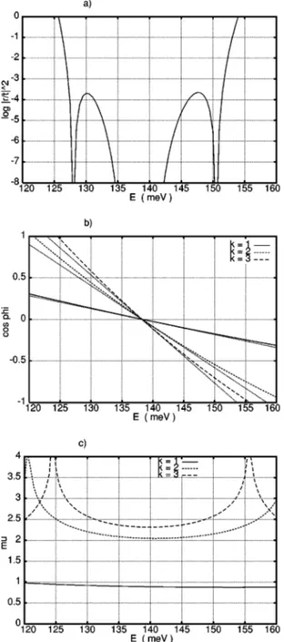
FIG. 4. Analysis of the 共adjusted兲 six-cell device of Coquelin et al. 共a兲 log兩r/t兩2,共b兲 cosk, and their tangents at the band center, and共c兲k.
21
TABLE III. Linear model solutions⌬kfor the N⫽7 filter.
k⫽ ⌬k k⫹1 Poissonk Poisson 0 0.125 0.125 0.166 0.166 1 0.2917 0.4167 0.298 0.464 2 0.2917 0.7083 0.268 0.732 3 0.1856 0.8939 0.160 0.892 4 0.07954 0.9735 0.072 0.964 5 0.02244 0.9959 0.0259 0.990 6 0.00379 0.9997 0.0077 0.998 7 0.000291 1 0.0002 0.998
For large p⬇N the linear model steps are exponentially small. Correspondingly, ⌬0⫽1/(N⫹1), which for N⬎4 greatly exceeds the value for the binomial or Butterworth filter, 2⫺N. The Poisson distribution Pk⫽ake⫺a/k! can be fitted by setting ⌬0⫽e⫺a to fix the mean value a. Alterna-tively we can choose a to give the second moment of the distribution of steps, as was done in the figure.
One conclusion we can draw is that a semiconductor bandpass filter should have many fewer cells than a similar optical or microwave filter. Most of the work will be done by the first few cells, so the later ones contribute less to the performance. This is useful information because it is easier to make a semiconductor device with fewer cells.
VII. EXAMPLE
On the web site of Gornik’s group in Vienna, Coquelin et al.8 presented an example of a six-barrier system which achieves 83% transmissivity over the first allowed miniband. The structure was modeled as a sequence of AlxGa1⫺xAs
quantum barriers with x⫽0.3, and GaAs wells. Viewed as a one-dimensional共1D兲 potential array, the barrier heights are 290 meV, and the widths were varied according to a Gauss-ian law,14taking the values 9, 28, and 40 Å. The well widths were set at 30 Å.
We can consider this an example of an ARC system with N⫽2 cells, surrounding two central cells X. We define a cell to consist of one barrier and a 15 Å spacer on each side of it. In our calculation, we took the effective mass at the conduc-tance band edge to be 0.092 and 0.067, respectively, and the energy gaps 1800 and 1424 MeV, based on Davies.22 We took account of energy dependence of the effective masses
FIG. 5. Analysis of the self-consistent N⫽2 ARC device derived from Coquelin et al.共a兲 log兩r/t兩2,共b兲 cos
k, and their tangents at the band center,
and共c兲k.21
FIG. 6. Pseudospin trajectories for the self-consistent N⫽2 device at three energies as labeled.
following the recipe of Nelson et al.16 Finally, following Pacher et al.7we took the barrier height to be 290 MeV. As a check of these parameters, we reproduced the five peaks shown between 128 and 160 meV in the figure of Ref. 8 for a periodic six-cell array.
Computing the Bloch phases and impedance parameters for each cell of their Gaussian array, one finds that every cell is a Bragg reflector close to the band center. The multi-Bragg character was improved by using 10 Å for the width of the weakest barrier and 15.05 Å for the corresponding half-well; with these small adjustments, the common Bragg point is at 138.3 meV. We will refer to this as the ‘‘adjusted’’ Coquelin array. The performance is illustrated in Fig. 4共a兲, where we plot兩r/t兩2for the entire device, on a natural log scale. This is a more sensitive presentation than simply plotting the trans-mission probability which would merely show a flat band with values at兩t兩2⫽1.
Thepare plotted21in Fig. 4共c兲; at the Bragg point they take values 0.580 : 1.623 : 2.319 which are very nearly in the ratio 1:3:4 of a classic Butterworth filter. However, moving away from the multi-Bragg point, the slopes of the cosp lines, seen in Fig. 4共b兲, are in the ratio 0.17:0.51:1.0 which is very far from equal slopes; indeed, rather close to the linear model.
Taking the parameters tp to be the above-mentioned slopes, and solving the stability conditions predicts that the
p should be close to those of the linear model, which are
1/3, 5/6, 1 times X. This suggests that improved perfor-mance should result from changing the barrier widths, to produce impedances which are consistent with the ensuing slopes.
Because the barriers are relatively high, the p are roughly proportional to the widths. Keeping the central cell parameters fixed (bX⫽40 Å), we found that with b1
⫽15.4 Å and b2⫽35.4 Å, the resulting p took values 0.893,2.052, compared to X⫽2.319, which are self-consistent with the solution of the stability equations using t1⫽0.24, t2⫽0.76. In Fig. 5共c兲 we show thek(E) across the allowed band. The values are quite flat in the center of the band, though all three curve upwards as the band edge is approached. It is not necessary for thekto be strictly con-stant; if their ratios are constant the spin analogy shows that the ARC mechanism will still work. The cospare shown in Fig. 5共b兲 along with the linear approximation from which the tpwere estimated. In Fig. 5共a兲 we show, on a log scale, 兩r/t兩2 for this solution. This is to be compared with Fig. 4共a兲, which used the共adjusted兲 Coquelin parameters. The average trans-missivity over the bandhas increased from 0.83 to 0.90.
In Fig. 6 we show the trajectories of the spin analogy, at three energies. In the first two cases 共near the band center兲 the spin orientation has indeed been moved to the pointX, and then back to the origin. This confirms that linear stability has been satisfied for the self-consistent filter. The third panel 共c兲 is at 150 meV, in a deep trough of 兩r/t兩2. The
perfor-mance is degrading and is only maintained because the ARC cells bring the spin to a point belowX, and the two central cells bring it 共almost兲 to the mirror image point above the axis. Then the downstream ARC cells can bring it back to OZ.
FIG. 7. Logarithmic plot of兩r/t兩2for N⫽2 ARC, with four and six central
cells, self-consistent solution.
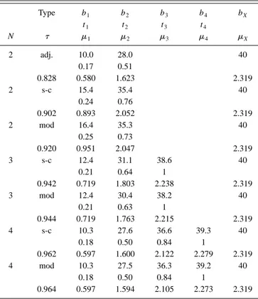
TABLE IV. Barrier widths, tpandpfor N-cell ARCs, both self-consistent
and modified fits.
Type b1 b2 b3 b4 bX t1 t2 t3 t4 N 1 2 3 4 X 2 adj. 10.0 28.0 40 0.17 0.51 0.828 0.580 1.623 2.319 2 s-c 15.4 35.4 40 0.24 0.76 0.902 0.893 2.052 2.319 2 mod 16.4 35.3 40 0.25 0.73 0.920 0.951 2.047 2.319 3 s-c 12.4 31.1 38.6 40 0.21 0.64 1 0.942 0.719 1.803 2.238 2.319 3 mod 12.4 30.4 38.2 40 0.21 0.63 1 0.944 0.719 1.763 2.215 2.319 4 s-c 10.3 27.6 36.6 39.3 40 0.18 0.50 0.84 1 0.962 0.597 1.600 2.122 2.279 2.319 4 mod 10.3 27.5 36.3 39.2 40 0.18 0.50 0.84 1 0.964 0.597 1.594 2.105 2.273 2.319
The performance should not depend on the number of central cells. This is true close to the design energy, but not further away, as seen in the previous paragraph. In Figs. 7共a兲 and 7共b兲 we show log兩r/t兩2for the same ARC with K⫽4 and K⫽6 central cells. Additional humps are seen, the number increasing like K, but always lying below some upper limit. This limit is related to the envelope of transmission minima, as discussed in Ref. 9. The width of the region with good performance widens slightly as K increases. Mostly this is the expected effect of the band edges becoming better de-fined by the central periodic structure. The transmissivity rises from 0.902 to 0.912 (K⫽4) and 0.915 (K⫽6), using the self-consistent N⫽2 parameters.
Some further improvement can be obtained by small variations in the parameters. Basically this involves a trade-off, making the inside humps of兩r/t兩2 a little higher and the outlying ones a little lower. One gains a bit on the width of the region of low reflectivity, while keeping the value under some maximum, say e⫺5. Our theory is based on assuming constant p and tp, but both of these break down as you move away from the multi-Bragg point. The small adjust-ments gain on the edges at the price of not hitting the target at the Bragg point. 共In optics or microwaves, such a fit is referred to as a Chebyshev filter. In our case of unequalp, one cannot use the Chebyshev polynomials, but rather the
intent, which is to widen the passband while maintaining a maximum value on the reflectance.兲 The best fit does depend on K because the humps that are being reduced have loca-tions which depend on K.
We conclude that the ARC obtained from solving the stability equations has improved the filter performance by about 10%, or close to half the gap from ideal performance, even for N⫽2 cells.
Further improvement is obtained by using a three- or four-cell ARC. The parameters of these ARC solutions are shown in Table IV. The barrier widths are in Å, while the other values are dimensionless. In all cases the well widths are 30 Å, except for the weakest barrier where 30.05 is main-tained. The difference between the self-consistent and modi-fied solutions is always small, but there is a gain in average transmissivity.
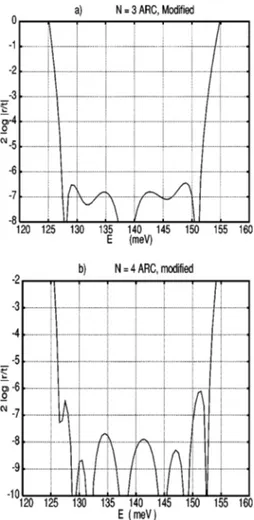
In Fig. 8 we show plots of log兩r/t兩2 for the modified solutions. They show that the filter bandwidth has increased as compared to the N⫽2 filter. Note the change of vertical scale between panels共a兲 and 共b兲 by a factor e⫺2.
VIII. CONCLUSION
We have used the analogy between potential scattering and precession of a spin-half system, to provide a simple and intuitive picture of the workings of a quarter-wave imped-ance transformer or passband filter. Based on this picture we have identified the stability conditions which take into ac-count the different rates of variation of the cosp with en-ergy. Enforcing these conditions makes an Nth order zero of the reflection amplitude for a system with an N-cell antire-flection coating. The rules for writing down these conditions are given in Appendix A.
Under the small-angle 共hyperbolic兲 approximation, the stability conditions become a set of N⫹1 linear equations for the impedance steps ⌬p. When the Bloch phases of the cells vary at the same rate, as in optical ARC’s, the solution of these equations is the well-known binomial filter, Eq.共19兲. For semiconductor superlattices, the rate of variation of the Bloch phases depends strongly on the strength of the poten-tial cell. A reasonable first approximation is provided by the linear model, in which tp⫽p. We have given the exact solu-tion of the linear model in Eq. 共28兲. As seen in Fig. 3, the steps of the linear model are close to a Poisson distribution, completely different from the Gaussian limit of the binomial distribution.
For arbitrary values of the tp, the stability conditions can be computed and the linear equations solved for the cor-responding⌬p. A numerical strategy for computing the co-efficient matrix is outlined in Appendix B. This allows for an iterative approach to the design of impedance filters. We have illustrated this process by finding a system similar to that of Coquelin et al. Their system was shown to be a But-terworth filter. By adjusting it to satisfy the stability condi-tions we improved the average transmissivity from 0.83 to 0.90 over the allowed band. Increasing the number of ARC cells provides further improvement.
FIG. 8. Logarithmic plot of兩r/t兩2for N⫽3 and N⫽4 ARCs, with
ACKNOWLEDGMENTS
We are grateful to NSERC-Canada for discovery Grant No. SAPIN-3198 共DWLS, GVM兲 and to DGES-Spain for continued support through Grant Nos. PB97-0915 and BFM2001-3710 共JM兲. We also thank Gideon Humphrey, holder of an NSERC SRA, for assistance with the calcula-tions and drawings. This work was carried out as part of CERION, Esprit project EP-27119 funded by the EU and NSERC.
APPENDIX A: GENERAL STABILITY CONDITION The stability condition of order m includes terms where some set k⫽k1,k2,...,kmof the tk’s replace the correspond-ing factors Uk in the expansion Eq. 共20兲. We define the re-sulting 1,2 matrix element contribution of this term as sinh(k1,k2,...,km), times the product of the corresponding tk, and with the requisite number of factors of⫺i. The case m⫽1 was treated in full in the main text, as was m⫽2. Learning from these examples we can state the general rule: The argument (k1,k2,...,km) involves a sum of the (⫺)p⌬p, each with its proper sign. If m is even, then the included terms are those between k1and k2⫺1, then from k3
to k4⫺1, etc. When m is odd, however, the first sum runs from p⫽0 to k1⫺1, and then successive groups run from k2 to k3⫺1, etc. In every case the last group ends at km⫺1. The reason is that removal of any of the Up matrices causes a glitch in the progression of signs, and with an odd number of glitches, the final entryXwill occur with the ‘‘wrong’’ sign. Then we must add ⌺ to removeX from the phase. Con-versely, with an even number of glitches we must subtract
⌺. Addition causes the first group of entries to be included
inwhile subtraction removes them.
We can now write down the general term in the expan-sion of the transfer matrix for N cells. The leading term is the product of sinptimes sinh⌺.关See Eq. 共20兲.兴 Dropping an overall phase, this contributes to the real part of r/t for the system. The m⫽1 terms, Eq. 共24兲, contribute to the imagi-nary part of r/t. In them, one of the sines is changed into a cosine; which is accounted for by the factor tp. In general, the odd-order corrections contribute to the imaginary part and the even order ones to the real part 共or vice versa de-pending on the parity of N). There are altogether N such correction types, which we call the stability conditions. Along with the normalizing condition 兺⌬p⫽X, they are sufficient to determine the values of the ⌬p ( p⫽0,1, . . . , N⫺1). This solution is valid over a range of energies where the tp vary linearly with energy around the multi-Bragg point. This allows the design of a generalized Butterworth transformer for application to electrons in semiconductors.
APPENDIX B: PROGRAMMING STABILITY EQUATIONS
The expansion Eq.共20兲 contains 2Nterms, which are in 共1,1兲 correspondence with the binary integers j ⫽关bNbN⫺1¯b1兴. 共The bq are binary bits.兲 Those j which have m nonzero bits contribute to the mth stability equation. For each bk⫽1, a factor tk is included in the coefficient.
We make the small-angle approximation sinh⬇. The stability equations reduce to the form
兺
p⫽0 N⫺1
C(m)p 共⫺兲p⌬
p⫽0, m⫽0¯共N⫺1兲. 共B1兲
Starting with j⫽0, up to 2N⫺1, each binary integer is parsed, assigned to class m, and the argument
(k1,k2, . . . ,km) is constructed as stated in Appendix A. Then for each of the⌬p occurring in, the coefficient Cp
(m)
is augmented by the product of tk, with k⫽k1, . . . ,km. In this way the N⫺1 stability equations can be constructed us-ing only N2 storage locations.
The j⫽0 term corresponds to the basic equation Eq. 共17兲 for ⌺⫽0. As m ranges over the values 0,1, . . . ,
N⫺1, we obtain N such equations, in the N⫹1 unknowns ⌬p. They are supplemented by the second equation in Eq. 共17兲, which normalizes the sum of the ⌬’s toX, and makes the system soluble.⌬Noccurs only in this extra equation, so one strategy is to solve the stability equations for the ⌬p, p⫽0,1, . . . ,N⫺1 in terms of ⌬N, and then use the last equa-tion to complete the soluequa-tion.
Obviously, as N increases, the time taken to accumulate the 2N contributions to the coefficients increases exponen-tially. Our code, written in C⫹⫹, works well up to N ⫽24. The method is general but for larger N one needs to use higher-precision integer representation for j. Fortunately, for the binomial and linear models, we have analytic solu-tions for general N, and these can be used to check the computer program.
1
R. J. Pegis, J. Opt. Soc. Am. 51, 1255共1961兲. 2E. Delano and R. J. Pegis, Prog. Opt. 7, 69共1969兲. 3P. G. Kard, Opt. Spektrosk. 2, 236共1957兲.
4H. J. Riblet, IRE Trans. Microwave Theory Tech. 5, 36共1957兲. 5R. E. Collin, Proc. IRE 43, 176共1955兲.
6
R. E. Collin, Foundations of Microwave Engineering共McGraw-Hill, New York, 1966兲.
7C. Pacher, C. Rauch, G. Strasser, E. Gornik, F. Elsholz, A. Wacker, G. Kiesslich, and E. Scho¨ll, Appl. Phys. Lett. 79, 1486共2001兲. See also C. Pacher et al., Photonics Spectra 12, 285共2001兲.
8
M. Coquelin, M. Kast, C. Pacher, G. Fasching, G. Strasser, and E. Gornik, Tech. Univ. Vienna 共unpublished兲; 具www.fke.tuwien.ac.at/transport/ transport.htm典.
9G. V. Morozov, D. W. L. Sprung, and J. Martorell, J. Phys. D 35, 2091 共2002兲; 35, 3052 共2002兲.
10T. K. Gaylord, E. N. Glytsis, and K. F. Brennan, J. Appl. Phys. 65, 2535 共1989兲.
11T. K. Gaylord, E. N. Glytsis, and K. F. Brennan, J. Appl. Phys. 67, 2623 共1990兲.
12
C. C. Chang and C. S. Kuo, J. Phys. D 32, 139共1999兲.
13H. H. Tung and C. P. Lee, IEEE J. Quantum Electron. 32, 507共1996兲; 32, 2122共1996兲.
14I. Gomez, F. Dominguez-Adame, E. Diez, and V. Bellani, J. Appl. Phys.
85, 3916共1999兲.
15Q. K. Yang and A. Z. Li, J. Appl. Phys. 87, 1963共2000兲.
16D. F. Nelson, R. C. Miller, and D. A. Kleinman, Phys. Rev. B 35, 7770 共1987兲.
17
At a band edge,diverges in such a way that⫺i sinsinh⫽M21has the correct value. A similar form for the transfer matrix holds in a forbid-den band. Bothandvary continuously across the band edge, where they become complex.
18J. J. Sakurai, in Modern Quantum Mechanics, revised edition, edited by S. F. Tuan共Addison-Wesley, Reading, MA, 1994兲, Chap. 3.
19D. W. L. Sprung, Hua Wu, and J. Martorell, Am. J. Phys. 61, 1118共1993兲. 20The Linear model is a rough approximation to the detailed behavior of the cosk, which captures the dominant trend that the phases for the stronger barriers vary much more rapidly than those of the weaker ones. It has the advantage of an analytical solution, from which one can draw general conclusions. In optics the corresponding approximation of constant indi-ces of refraction leads to the binomial filter design.
21In a forbidden band,
k→k⫾i/2; the disjoint line segments below 125 meV and above 156 meV arek.
22John H. Davies, Physics of Low-dimensional Semiconductors共Cambridge University Press, Cambridge, England, 1998兲.
23W. H. Press, S. A. Teutolksky, W. T. Vetterling, and B. P. Flamery,
Nu-merical Recipes in C共Cambridge University Press, Cambridge, England,