A bit of Keynesian debt-to-GDP arithmetic for
deficit-capped countries
STEFANO DI BUCCHIANICO
Abstract: This paper expands some recent Keynesian debt-to-GDP
arithmetic exercises in three respects. Firstly, it analyses the output and capacity losses associated with a ‘balanced budget’ fiscal policy. Secondly, the possible Keynesian features of a policy looking at the difference between the growth rate and the interest rate are also discussed, showing a condition which allows for a debt-to-GDP ratio reduction via primary deficit spending. Lastly, the minimum necessary fiscal multiplier values needed to make austerity policy counterproductive are calculated for the PIGS economies covering the 1998 – 2018 period. The results show the substantial case for the Keynesian arithmetic to hold.
Keywords: Public debt, debt-to-GDP ratio, fiscal policy, fiscal multiplier JEL Codes: E62, H62, H63
INTRODUCTION
Since the eighties, one of the most harshly debated topics regarding the strategies to conduct economic policies, especially in developing countries, has been the so-called ‘Washington consensus’. As reported in Mavroudeas and Papadatos (2007), among the prescriptions of paramount importance within that kind of policy agenda (such as trade liberalization, exchange rate competitiveness, privatization of public utilities, etc.), fiscal discipline used to rank in the first positions. It is already more than two decades since the latter recommendation has become protagonist of discussions in the Eurozone as well, particularly after the 2011 crisis. While the limitations to public expenditure were already in place with the famous parameters of the 1992 Maastricht Treaty, in 2012 the Fiscal Compact has considerably reinforced their strictness. From a 3% deficit/GDP ratio, the limit has been narrowed down to almost zero, and the debt/GDP ratios exceeding the well-known 60% threshold ought to be reduced over a 20 years horizon. * Department of Economics, Roma Tre University (e-mail: [email protected])
The debate has focused, among other things, upon the role of those parameters in the Eurozone crisis (which has followed the US Great Recession) and the effectiveness of the ‘austerity’ agenda in solving it. The discussion of the Eurozone case may be carried forward by touching upon many facets, such as the viability of the Euro currency area (Barba and De Vivo 2013), the interpretation of the crisis as a balance-of-payments or a monetary sovereignty issue (Cesaratto 2017), and so forth. What we want to linger on is the apparently unescapable recommendation to lower the debt-to-GDP ratio. We will not question whether its reduction can per
se be beneficial for an economy, neither whether some specific values for
the debt and deficit to GDP ratios have reasons to be of utmost relevance for economic policy. Rather, from a Keynesian standpoint in which the State spends first and collect taxes after (Cesaratto 2016), we will try to analyse how the deficit caps can shape economic policies, whether there might be a compromise between them and a Keynesian-inspired public spending policy, and what are some of their medium-run consequences. In particular, this contribution aims on one hand at integrating the critical considerations of Alexiou (2011) about the ‘deficit paranoia’ and its unfavourable effects on unemployment, and the ‘Keynesian recovery policy’ described by Fiorentini and Montani (2018) for the European Union, which is the opposite of what is currently being pursued.
The work is structured in the following manner: Section 2 briefly reviews the main competing visions about the role of public expenditure and some empirical debates about the effectiveness of austerity policies and the value of the fiscal multiplier; Section 3 utilizes a stylized Keynesian arithmetic to understand whether deficit-capped policies can be useful in lowering the debt-to-GDP ratio and the medium run effects of these actions in terms of output, capacity build-up and employment; Section 4 analyses the minimum values for the fiscal multipliers in the Eurozone periphery that make austerity policies counterproductive in light of the reduction of the debt-to-GDP ratio are calculated; Section 5 concludes.
THE DEBATE ABOUT AUSTERITY
Two main approaches can be recognized in the literature on the effectiveness of the austerity policies targeted at slashing public expenditure and curbing public debt accumulation. On one hand we find the neoclassical vision, according to which public debt accumulation is detrimental to growth. Specifically, the issuance of public debt to finance State expenditure causes the emergence of the ‘crowding-out’ phenomenon, whereby a higher public
expenditure causes a rise of the interest rate which discourages private investment (Hall 2009).1 Moreover, a deficit-financed public expenditure policy is subject to the ‘Ricardian equivalence’ theorem, according to which the expected future rise of taxes (allegedly needed to pay down the new debt) makes agents willing to save out of their income already in the current period (Barro 1989). Given that economic growth, according to this view, is mainly determined by supply side factors such as population growth and technical progress, the best policy to follow would be to reduce to the minimum the utilization of public expenditure and the accumulation of public debt. The difference between the main proposers of this view rests on the attitude towards the short period: while Real Business Cycle scholars do not allow for exceptions, the New – Keynesians are more inclined to preserve some Keynesian features due to price rigidities.
On the other hand, there are approaches sharing the so-called ‘Keynesian hypothesis’, according to which investment is independent from prior savings both in the short and long term. In this way, the ‘principle of effective demand’, which is one of the most important analytical discoveries made by Keynes (1936), can be fruitfully employed to analyse not only current production levels but also growth. In this case, contrary to the neoclassical vision, public deficit-financed expenditure is one of the most important tools capable of injecting new purchasing power into the economy without subtracting resources from other employments. Nonetheless, we will not be engaged here in a discussion of the different strands of thought sharing the ‘Keynesian hypothesis’; among them we can list the post-Keynesian, neo-Kaleckian and Sraffian strands of thought (Cesaratto, 2015). We will not discuss the position of Keynes himself about public debt accumulation either, despite one may say he used to be prudent in that respect (Aspromourgos, 2014b).
Nevertheless, while these broad groups confront themselves on the ultimate determinants of accumulation and growth, we are mainly interested in seeing the issue from a narrower perspective. In other words, given that we want to put the attention on some of the consequences of the deficit-cap policies on the debt-to-GDP ratio, our focus can be directed to the debate about the effectiveness of austerity policies in terms of the value of the fiscal multiplier.2 As we will see in Section 3, one way to evaluate the effect of public spending on the debt-to-GDP ratio is to look at the size of fiscal multiplier, because a given deficit-financed outlay can either make that ratio rise or fall according to whether the multiplier is respectively lower or higher than certain thresholds. In general terms, the
lower the multiplier the more the arguments favouring austerity gain credibility. The debate has seen, especially during the nineties, a neat preference for austerity, particularly for the ‘expansionary austerity’ version, which practically assigned to the fiscal multiplier a negative value, stating that a fiscal retrenchment would cause GDP to grow. Among others, the contributions of Alesina and Perotti (1995), Giavazzi and Pagano (1990, 1995) stand out as particularly adamant in the support of austerity. Afterwards, the period following the 2009 US Great Recession and the 2011 Eurozone crisis has seen a considerable upward revision of the overall assessments of the fiscal multipliers’ size. For a reconstruction of the debate up to this point, see Nuti (2013a) and Cozzi (2013). Among others, Perotti (2004), Christiano et al. (2011), Furceri and Mourougane (2012) find values which are consistently above unity. Along with the empirical contentions, there are also theoretical debates. Boyer (2012) provides a recount of the shortcomings of the austerity framework, finding fallacies in considering the crises of those years due to excessive public spending, in the underestimation of their demand-side effects and the overestimation of the Ricardian equivalence effects, and in the neglect of the different socio-institutional contexts that render each country unique and not subjectable to a standardized restrictive policy. Moreover, Foresti and Marani (2014) contend that austerity cannot be generally considered a viable policy since its supposed desirable effects on growth and public finances are likely to come about only in very peculiar situations.
A very recent thread of literature is now trying to bring the austerity programme back to the fore, but in a somewhat milder version. According to Alesina et al. (2015, 2018) and Alesina et al. (2017), an austerity programme ran through a reduction in public expenditure is likely to be successful, since it entails a negligible output loss. A reduction via tax increases, on the contrary, is said to be liable to increase the debt-to-GDP ratio because of the adverse effect on output. On the contrary, Botta and Tori (2018) offer a comprehensive theoretical and empirical test for the predictions of the austerity advocates, and state that what must be expected is that they produce perverse effects.
DEFICIT CAPS AND THE DEBT-TO-GDP RATIO
In this section we will be engaged in a theoretical discussion about the relationship between public expenditure and the debt-to-GDP ratio. We are going to split the analysis into three parts. The first and second parts will present, from different viewpoints, a ‘compatibility’ scenario. We will ask
ourselves whether it is possible, despite the adherence to the Keynesian perspective, to pursue a policy of debt-to-GDP reduction by sticking to a no-deficit rule. We will therefore be mostly interested in the short-run effects of a deficit-cap on the debt-to-GDP ratio. In the third part we will look at the possible effects upon employment and capacity formation of an attempt to reduce that ratio by means of a balanced budget strategy.
Relative Effects of Deficit Spending on Public Debt and Gdp In this part we will look at the effect of deficit spending constrained by a zero-deficit rule by assessing its effect on both public debt and GDP. Leão (2013, pp. 452 – 453) proposes a simple but insightful arithmetical exercise showing the condition under which an expansionary fiscal policy can lower the debt-to-GDP ratio. He starts from the accounting of a GDP increase due to the fiscal multiplier m times the variation in public expenditure G:
(1) and of a public debt increase due to the public spending variation minus the net taxes response coefficient (difference between the tax t and transfers
tr responsiveness to output) times the output change:
(2) In his proof the ratio falls provided that
(3) in other words, if the initial debt-to-GDP ratio B/Y exceeds the incremental debt-to-GDP ratio associated with an increase in public spending ΔB/ΔY. The crucial finding is that the latter situation materializes when
(4) so, when the initial debt-to-GDP ratio exceeds the inverse of the fiscal multiplier minus the (net) tax responsiveness to output. Indeed, in the author’s proof it is shown that condition (4) lets the growth of GDP more than outweigh the growth in public debt. It is therefore possible to state that in a Keynesian line of thought, for a sufficiently high fiscal multiplier, an autonomous public spending impulse can be beneficial considering the debt-to-GDP ratio reduction target.
thereby posing an obstacle to such a strategy. Our question is now: is it possible to reduce the debt-to-GDP ratio via a Keynesian policy of increasing expenditure without violating those European rules? We are going to prove that the answer can be yes, although not without considerable costs in terms of output and employment. In other words, we will try to pinpoint what may be termed the least Keynesian policy conceivable. To such an end, we refer to the principle of the ‘balanced budget’ theorem of Haavelmo (1945), with some refinements about the role of the tax structure from Salant (1957). For instance, Zezza (2012, pp. 44 – 51) started from similar considerations upon the possibility to lower the debt-to-GDP ratio by keeping the budget balanced, but then developed his argument by pointing the attention towards the role of income distribution and external imbalances in connection with fiscal austerity.
The theorem showed how it is possible to increase the GDP by the same amount in which public spending is increased, without increasing public debt, since the autonomous increment in public expenditure is matched by an equivalent autonomous taxation increment. Though, in our framework we will slightly modify the reasoning. We are going to develop it by taking the increase in public expenditure as given and varying the tax and transfer rates. We also consider the interdependence between the fiscal multiplier and the tax structure required to ensure a balanced budget. Consistently with equation (2), we start from tax schemata in which the endogenous components of taxation and transfers act as an automatic stabilizer, in order to mimic a governmental usage of the endogenous component of transfers as a countercyclical tool:
(5) and then we explicit the two equations system for the change in output and public budget:
In equation (7), for a given variation in public expenditure we derive the condition needed to balance the budget:
(6)
(8) Since c (0 < c < 1) is exogenously fixed and is taken as given, by setting one tax parameters the system is closed. Equation (8) shows that the appropriate combination of parameters requires that the sum of the tax and transfers marginal rates has to be equal to 1. In equation (6) this means that, for a given marginal propensity to consume, the fiscal multiplier is 1 as well. The condition in equation (3) for a debt-to-GDP ratio decrease in this perspective simply becomes
(9) and therefore, for whatever initial debt-to-GDP ratio, a ‘balanced budget’ fiscal policy would lower it, since the numerator does not change, while the denominator increases. This straightforward result becomes in our opinion interesting compared to the claims of Codogno and Galli (2017, Sec. 3, pp. 15 – 17). As we will discuss below, Codogno and Galli argue in favour of fiscal retrenchments when the economy is not in deep recessions, and state that fiscal austerity is generally a virtue. The authors maintain that it is not possible to have a self-financed fiscal spending in which the initial deficit impulse is offset by the feedback effect on taxes, unless the marginal tax rate takes up an absurd 100% value. For the latter reason, they also add that the fiscal multiplier cannot be high if such a policy is introduced. In our opinion, on the contrary, it is possible to handle the issue differently when, together with the taxes, a transfer component of fiscal policy is inserted. As shown, the positive effect of the initial deficit expenditure on income levels consents on the one hand to collect more taxes, and on the other hand to reduce the endogenous transfers outlay. For this motive, the balanced-budget policy is viable without the need to suppose a one-for-one increase in the marginal tax rate. However, we agree with Codogno and Galli on the consequence of that policy on the value of the multiplier. Our take on this fact is anyway opposite: even though the deficit cap imposed upon the public sector appears prima facie to be compatible, as we have just seen, with a reduction in the debt-to-GDP ratio, this does not mean that, from a Keynesian point of view, it should be welcomed. Indeed, Palley (2012, pp. 98 – 100) shows that the deficit caps imposed by the Maastricht
Treaty or the Fiscal Compact prevent the public budget from being an automatic stabilizer, or worse they turn it into an automatic destabilizer. This happens because the amount of spending allowed when an adverse shock hits the economy becomes pro-cyclical, since the expendable quota of GDP is exogenously fixed. Ribeiro and Lima (2018), in a similar fashion, show that setting a limit to public spending of this kind does not guarantee a public debt-to-GDP ratio non-explosive trajectory. Such a conclusion holds specially for countries facing high interest payments and regressive taxation systems. Further, the authors maintain that the deficit cap is likely to reinforce the stability conditions of the debt-to-GDP ratio, but in countries where its stability is already in place.
In our case, since we let GDP growth depend exclusively on exogenous government decisions to spend, there is no exogenous shock. Rather, the spending decision is subject to a deliberate commitment, not to let the public debt augment. An example of such a policy commitment is described in Cesaratto and Zezza (2018). They analyse the case of Italy, which has throughout the years progressively abandoned an active employment sustain policy in favour of ‘external’ discipline aimed at slashing inflation, thus following the spirit of the European treaties. In the same way, Storm (2019) attributes the economic decline witnessed by the Italian economy in the last three decades to a perpetual public sector spending kerb, together with the overvaluation of the exchange rate and the income distribution being unfavourable to low-income classes. In this respect, therefore, rather than gauging the role of stabilization of the public budget, it is possible to reinterpret the progressive adhesion of the Eurozone economies to the mentioned treaties as a new phase in the public policy drafting. In the line of reasoning of Ciccone (2013), whose scope was to study how a public expenditure policy shift affects the debt-to-GDP ratio, we can make an evaluation between two different policies, the base case versus an alternative restrictive policy. So, the restrained policies under the Maastricht Treaty/Fiscal Compact rules can be labelled as restrictive when compared to the unconstrained ones previously applied. Equation (8) can then be reformulated to deliver a positive increase in the overall public budget variation in equation (7) by setting:
The sum of the tax and transfer marginal rates is now strictly lower than 1, and this leads to a multiplier higher than 1, a higher output for a given public expenditure stimulus and a positive increment for the public debt. We can therefore explicit the difference in output growth between
the two policies as the difference between two fiscal multipliers times the given public spending variation
(10) In (10) the percentage output loss arises since the unbalanced budget (UB) multiplier is higher than the balanced budget (BB) one, and this is due to the commitment to the no-deficit rule. Thus, the attempt to lower the debt-to-GDP ratio by means of a balanced budget policy design can be successful, but nonetheless causes realized output to be lower than the one otherwise obtainable. See Uxó et al. (2018) for the application of this type of reasoning to the Spanish case in recent years.
COMPARISON BETWEEN GROWTH RATE AND INTEREST RATE
While in the preceding subsection we have lingered on the study of the subject by means of the relative comparison of a deficit spending policy on both GDP and public debt variations, we will now look again at the topic from a different angle. The considerations we are going to develop can add to the debate about deficit sustainability which has seen, among others, two recent contributions by Krugman (2019) and Blanchard (2019). They both stress the viability of fiscal deficits for the US since the difference between the growth rate of the economy and the interest rate on its public debt has been historically positive; the more so in the last decade, because of ultra-low interest rates. Let us expand the general argument to be made about the relevance of that difference in light of public debt sustainability. A standard arithmetic of the public debt sustainability looks at the difference between the economy’s growth rate and the interest rate to assess what is the fiscal policy stance that keeps the debt-to-GDP ratio stable at its initial level:
In (11) b is the public debt in percentage of GDP, i is the nominal interest rate, g is the nominal GDP growth rate, d is the primary deficit in percentage of GDP. Below we will also use d*, the total deficit in percentage
of GDP. By imposing the constancy over time of the debt-to-GDP ratio, one obtains after some simple manipulations the conditions in (12), where d (11)
can be now read as the primary deficit that stabilizes that ratio. For a certain initial b, once the difference between the given growth rate and interest rate is calculated, one can also gauge which fiscal stance ought to be implemented in order to keep that ratio constant.
The imposition of austerity measures that have been justified recurring to this kind of accounting has already been starkly criticized by Pasinetti (1998). The author, by employing the difference between the interest rate and the growth rate (i – g), contends that the Maastricht Treaty 3%-cap is senseless. That judgement is driven by the following reasoning: once the
i-g differential is calculated, there is a well-defined, continuous relationship
between the initial debt-to-GDP ratio and the sustainability primary surplus/ deficit. The same holds for the total deficit once the growth rate of the economy and the initial debt-to-GDP ratio are available. Let us illustrate the argument of Pasinetti, drawing his graphs in terms of equations (11) and (12):
Figure 1 – Sustainability area for the total deficit/GDP ratio. Source: own elaboration on Pasinetti (1998).
Figure 2 – Sustainability area for the primary deficit/GDP ratio. Source: own elaboration on Pasinetti (1998).
In Figure 1, given a positive growth rate, the sustainable deficit d* is a
growth rate is higher than the interest rate, the same holds for the primary deficit. In other words, choosing a single, fixed value for the primary and/or total deficit neglects the fact that the sustainability condition is not verified in a single point, but in an area. Obviously, this kind of criticism holds equally well for a deficit-cap of the magnitude of the 3% as for one placed at the 0%. However, Pasinetti both leaves untouched the issue of what is the relationship to be expected to normally exist between the rate of growth and the rate of interest and takes the growth rate of the economy as given for the sake of deriving the sustainable deficits.
Aspromourgos et al. (2009, Sec. 3, pp. 438 – 440) discuss the former point, among other things. According to mainstream theory, the relationship between the interest rate and the growth rate of an economy ought to be well-defined by the ‘dynamic efficiency’ condition i > g. Following this, the interest rate is bound to be, in the long-run, equal or higher than the growth rate, in order to ensure that per-capita consumption is optimally allocated through time. Nonetheless, as the authors maintain, the results of the ‘Cambridge Capital controversies’ showed the impossibility to evaluate that difference has a measure of inefficiency, as there is no definite relationship between a steady-state value for the interest rate and the per-capita consumption made possible by a certain propensity to save. Hence, the interest rate and the growth rate can undertake different paths, which are not bound to get back in the longer term to the ‘dynamic efficiency’ position. With respect to the other issue, Aspromourgos (2014a, Sec. 2, pp. 575 – 582) develops an analysis that couples full-employment growth and public debt sustainability, linking the two within a super multiplier framework. In order to derive a condition that satisfies both requirements, the author imposes that public spending must grow at the same exogenous rate of labour supply. This hypothesis allows, once again, to employ (12), because for a certain exogenously given growth rate, when the interest rate is given as well, the sustainability public primary surplus/deficit can be calculated.
What we want to add to these insightful analyses is the attempt to evaluate which fiscal policy might be utilized in order to make the debt-to-GDP ratio constant once it is acknowledged that, as in Pasinetti (1998), the rationale for imposing the deficit-cap is flawed, and, as in Aspromourgos et
al. (2009), there is no straightforward relation among i, g and b. We propose
to look at the growth rate g itself as a variable which is liable to be directly affected by the fiscal policy stance. Therefore, we will directly compare the growth rate determined by fiscal policy and the interest rate, rather than looking at their difference in order to understand what primary surplus/
deficit is needed to make the debt-to-GDP ratio sustainable.
The debt-to-GDP ratio falls when the difference g – i is positive. We then have to formalize the growth rate of the economy by making it depend only on the deficit spending. Hence:
In (13) we find all the variables thus far employed, plus m1 and m2 which are respectively the fiscal multiplier associated to the primary deficit and the fiscal multiplier of the interest payments on public debt. Isolating d in (13) yields:
Equation (14) tells us that in order to run a primary deficit that lowers the debt-to-GDP ratio it suffices that:
� the multiplier of the interest payments on public debt is lower than the inverse of the debt-to-GDP ratio;
� the multiplier of general public expenditure is strictly positive. These conditions appears to be rather slack. Taking for granted the positivity of the fiscal multiplier, we find it reasonable to think to a value of 0.5 for the interest payments multiplier as being quite high. However, such a value would require a higher than 200% debt-to-GDP ratio (GDP-to-debt ratio < 0.5) to make a primary surplus needed. We think that this result can be of interest because it complements others similar that look at the comparison between the value of the multiplier and the value of the debt-to-GDP ratio, such as Ciccone (2013), Leão (2013), Nuti (2013b). However, our outcome highlights the role of a specific kind of expenditure. The latter is likely to be relevant when looking at the sustainability issue from the point of view discussed in the present section, since highly indebted countries are usually bound to incur in higher interest payments out of their public debt. Furthermore, a higher value of the fiscal expenditure multiplier lowers the value of the sustainability primary deficit, since a certain outlay can generate higher final demand. On the contrary, a higher rate of interest
calls for a higher primary deficit. It is true that higher interest payments add to final demand, but with a multiplier so low that it usually cannot compensate for the heightened level of the debt-to-GDP ratio that they cause. However, rather than curbing the amount of primary expenditure, this effect makes the need for a primary deficit that boosts GDP growth more than the interest component more pressing. Thus, if condition (14) is valid, a fiscal rule that fixes once and for all the value of the total deficit to zero can impede the achievement of the required primary deficit, since an increasing quota of the total is taken up by the debt servicing when the interest rate rises.
The losses from getting to and staying at a balanced-budget Generally speaking, it is very likely that a country cannot simply adhere to a zero-deficit policy, but it needs a certain time span to get to fulfil that type of policy. In this subsection we will have a brief look at some possible undesirable side-effects of the balanced budget policy which do not directly impact the debt-to-GDP ratio.
Firstly, we look at the employment outcome of a policy trying to balance the budget. In this way we attempt at providing a clue about the employment losses arising during the path towards the zero-deficit goal. In order to show the point, we rely on the input-output analysis upon Portugal carried out by Lopes and do Amaral (2017). The authors start from the input-output relationships of their country to show how fiscal retrenchments can have several adverse repercussions on the economy. Of particular interest to our eyes is the unemployment/budget balance trade off (2017, pp. 79 – 82), which is built on these premises:
In (15) Y is GDP at market prices, C private consumption, G public consumption, I total investment, Ex exports, while vaC, vaG, vaI, vaEx are the
coefficients representing the value added content of each variable, that are derived from a Leontief model (2017, Appendix 1, p. 89). Equation (16) describes the government budget B, where t is the average tax rate, O the net government receipts including public debt interest, IPub is public
investment, TR transfers. Equation (17) describes private consumption as a function of n, the average propensity to consume, and Yd, the disposable income. In (18) we find the consumption function in which the relations in (16) and (17) are utilized. Once (18) is plugged into (15) one obtains:
By substituting (19) in (18), the two economists obtain a function of consumption related to the budgetary stance C(B):
In (20), ceteris paribus, they can see how fiscal policy can contribute to private consumption levels. In order to relate that function to the employment level, they introduce the employment function:
in which lC, lG, lI, lEx are the labour coefficients tied to each demand element. Finally, by replacing (20) in (21) they arrive at:
which displays the employment/budget balance inverse relationship. In fact, in (16) a total public expenditure higher than tax collection generates a deficit which adds to final demand. Then, via the rather cumbersome process depicted by the input-output relations, it fosters labour employment. In this respect, a policy geared towards a zero-deficit not only adversely impacts income prospects, but also seriously undermines the attempt to get to full employment. In the specific case analysed by the two economists, a zero-deficit policy would have caused in 2011 in Portugal a short-run rise of unemployment of about 4.5%, given the input-output relations shaping the Portuguese productive matrix at that time.
Secondly, we want to make a point about the possible long-run effects of a zero-deficit policy on capital accumulation. Therefore, while in the preceding part we have been busy showing the effects on employment arising while getting to the target, we now try to envision how this policy affects the economy when it has been in place for a while. Ciccone (2013, pp. 29 – 33), after the assessment of the adverse effect on output and the debt-to-GDP ratio of a more restrictive policy, analyses its harmful impact on private investment as well. Considering the strong dependence of the latter upon the recent and foreseeable levels of aggregate demand, which
is in turn directly affected by government decisions about the levels of public spending, the author argues that the restrictive policy will result in a further depressive effect on total demand via its curbing power upon private decisions to invest. Thus, drawing on Garegnani (1992, pp. 50 – 53), we can roughly calculate how the output loss in (10) will not be limited to its single-period effect, but is liable to cause a permanent potential capacity loss, which can in turn be linked to the foregone investment flows caused by the restrictive policy. In fact, Garegnani argues, even a single-period capacity underutilization can result in a foregone current production plus a foregone capacity build-up. The latter is due to the missed possibility to stimulate investment by intensively using the available capacity and thus kick-starting a virtuous multiplier-accelerator interaction. This kind of counterfactual exercise rests on the idea that even a single-period demand restraint results in an output loss. The latter, when cumulated, can result in an ever-increasing gap between what is and could be potentially produced and what could have been produced were the economy always appropriately stimulated via aggregate demand policies. We thus exploit his formula for such a capacity loss
(where x is a percentage output loss, y is the normal output-capital ratio, s is the propensity to save, t is the time horizon covered by the calculation) to connect it to our argument. To give an order of magnitude, we can suppose that with a 0.5 difference between the UB and BB multipliers, a single year 1.45% percentage output loss as defined in (10) can lead to a cumulative 0.9% lost capacity (CL) over a 5 years horizon. It is important to highlight that such a capacity loss arises owing to the supposition of a government trying to cope with a deficit cap set to zero. As seen, such an attempt requires a lower than otherwise attainable fiscal multiplier. But, in addition to this, there is also the capacity loss already in place given the impossibility to implement a positive deficit spending plan. Hence, an ulterior 1.8% capacity loss following a single year 3% output loss, which follows from the difference between the 3% deficit allowed by the Maastricht Treaty and the 0% entailed by the Fiscal Compact, is already in place (all the derivations are in Appendix a).
Along these lines, Fontanari et al. (2019, Sec. 5, pp. 32 – 36) provide an estimation of what they call a ‘high demand potential path’. This is defined as a counterfactual regime in which, were unemployment kept continuously at a very low level via appropriate aggregate demand
stimuluses, the US economy would not have suffered a cumulated loss of income and capital formation due to periods of weak growth. From our viewpoint, regimes in which the public sector contribution to aggregate demand formation are curbed by deficit-caps impositions cannot but generate lower-than-possible income levels, which subsequently translates into lower potential growth. These considerations are again at odds with Codogno and Galli (2017, Sec. 6 – 7 – 8, pp. 24 – 34), who albeit accepting the perverse effect of austerity in the short run, revert to a mainstream treatment of the long term. In their opinion indeed, continuous deficit spending is not sustainable and the ‘hysteresis’ effects analysed by, among others, DeLong
et al. (2012) are bound to be valid only in the case of deep recessions and
with a monetary policy constrained by the ‘zero-lower-bound’. Nevertheless, it seems clear that the substantial difference distinguishing the two approaches to the issues we have been treating is the viewpoint concerning their long-haul impacts. Indeed, while the short run outcomes appear to be unambiguously deemed as adverse, the possibility to envision a longer-term reverse to a full-employment situation is crucial. In our opinion, despite the fact that a treatment of the long term is beyond the scope of the present piece, the increasing part of the mainstream literature devoted to hysteresis and permanent effects of fiscal consolidation (Fatás and Summers, 2018) testifies the spreading awareness about the dangerous effects of a lack of aggregate demand for the potential output itself.
AN EMPIRICAL EVALUATION
In this section we will investigate the empirical relevance of the Keynesian argument that prescribes to lower the debt-to-GDP ratio via deficit spending, particularly in the formulation looking at the value of the fiscal multiplier (cf. subsection 3 above). We will accordingly calculate the multipliers that verify the conditions therein explained. However, it is important to notice that what we will be engaged with is neither an econometric estimation nor a model simulation. Therefore, it can only offer indicative values for our variables of interest. Leão (2013, pp. 456 – 463), grounding on equations (1) to (4), derives an operational ‘rule-of-thumb’ to ascertain whether austerity is counterproductive or not in light of the debt-to-GDP reduction target:
are higher than the sum of the initial debt-to-GDP ratio and the total tax responsiveness to output, than an austerity measure (a public expenditure reduction entailing a budget negative variation) can be expected to increase that ratio.
After calculating the parameters to the right-hand side of the inequality and comparing the results with the multipliers from the empirical literature, the author concluded that in France, Germany, UK and USA the respective debt-to-GDP ratios in 2012 would have been augmented by austerity policies. In fact, m was found to be higher than the minimum value involved by equation (24). We will try to widen those findings in two respects: pointing the attention to the so-called PIGS economies (Portugal, Italy, Greece, Spain) and enlarging the vector of results.3 The choice of the countries to examine has been dictated by the wish to detect the potential effectiveness of austerity measures in economies that have been mostly hit by those policies, at least in the European Union. The enlargement of the time horizon reflects the desire to provide a glance also upon a longer time span. The calculation procedure, described in Appendix b, delivered the following values:
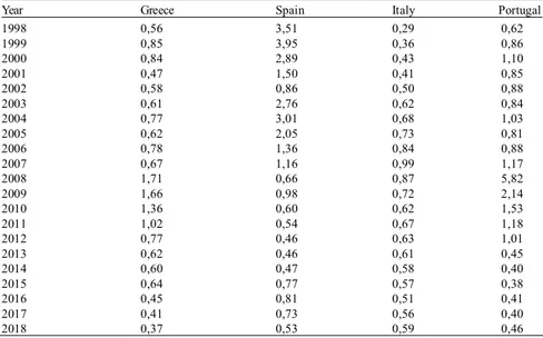
Table 1 – Minimum values for the fiscal multiplier that make an austerity policy increase the initial debt-to-GDP ratio. Source: own elaboration.
Year Greece Spain Italy Portugal
1998 0,56 3,51 0,29 0,62 1999 0,85 3,95 0,36 0,86 2000 0,84 2,89 0,43 1,10 2001 0,47 1,50 0,41 0,85 2002 0,58 0,86 0,50 0,88 2003 0,61 2,76 0,62 0,84 2004 0,77 3,01 0,68 1,03 2005 0,62 2,05 0,73 0,81 2006 0,78 1,36 0,84 0,88 2007 0,67 1,16 0,99 1,17 2008 1,71 0,66 0,87 5,82 2009 1,66 0,98 0,72 2,14 2010 1,36 0,60 0,62 1,53 2011 1,02 0,54 0,67 1,18 2012 0,77 0,46 0,63 1,01 2013 0,62 0,46 0,61 0,45 2014 0,60 0,47 0,58 0,40 2015 0,64 0,77 0,57 0,38 2016 0,45 0,81 0,51 0,41 2017 0,41 0,73 0,56 0,40 2018 0,37 0,53 0,59 0,46
The outcomes reported in Table 1 ought to be interpreted as an answer to this question: what is the minimum value for the fiscal multiplier in a given year from 1998 to 2018 for each of the countries examined that, given its initial debt-to-GDP ratio and the tax and transfers responsiveness
to output, makes a negative public budget balance increase the debt-to-GDP ratio? Yet, without a reference value for what the fiscal multiplier may be expected to be, those numbers are clueless.
For the sake of carrying out a comparison, we deploy the fiscal multipliers values reported by Gechert and Rannenberg (2018) from a meta-analysis aimed at scrutinizing the available literature on the fiscal multipliers’ size. This study refines and updates the findings of Gechert (2015) about the value for fiscal multipliers of several spending categories (generic, public investment, transfers, taxes etc.). The principal novelty with respect to the 2015 work is constituted by the addition of the indication about how fiscal multipliers differ amongst periods in which the economy is in a bad, average or good scenario. For the sake of extracting a multiplier value which is compatible with our empirical exercise, we have selected from Gechert and Rannenberg (2018, p. 1170, Table 5, column 1) the coefficient relative to an ‘unspecified’ public expenditure category for an ‘average’ economy’s performance from a ‘base case’ estimation procedure: m = 0,88. We have then sorted the cases presented in Table 1 in two broad categories: the entire sample, and the subsample relative only to the post-crisis period, which we have identified as the years from 2010 to 2018. Within these two samples, we have defined three instances: the ‘strongly Keynesian’ cases (minimum multiplier lower than 0,88), the ‘Keynesian’ cases (minimum multiplier lower than the 1,2, a value chosen by augmenting the previous by one-third), and the ‘austerian’ cases (minimum multiplier higher than 1,2). The results are:
Table 2 – Minimum fiscal multipliers values sorted out by ranges of magnitude for both the entire sample and the post-crisis subsample. Source: own elaboration. Full sample (1998 – 2018, 84 obs.) Post-crisis subsample (2010 - 2018, 36 obs.) Min m value N° of cases Percentage Min m value N° of cases Percentage
m < 0,88 59 70% m < 0,88 31 86%
m < 1,2 70 83% m < 1,2 34 94%
m > 1,2 14 17% m > 1,2 2 6%
As one can see, the ‘strongly Keynesian’ case captures the 70% of the total cases and the 86% of the post-crisis cases. The ‘Keynesian’ case, which cumulates the previous ones and the episodes when a higher multiplying value is needed, covers the 83% of the total sample, and the 94% of the post-crisis sample. Obviously, the remaining cases fall into the ‘austerian’ category: they signal the possibility to lower the debt-to-GDP ratio via austerity measures. Yet, the latter can be deemed to be counterproductive in the bulk of the cases under enquiry. Moreover, the
threshold value that signals the ‘strongly Keynesian’ case has been chosen to provide a prudent value: as we will see below, the multiplier values might be considerably higher.
The results appear compatible with the data for the debt-to-GDP ratios of the PIGS countries for the 2010 – 2018 time span, which have witnessed a dramatic rise from their respective initial values:
Figure 3 – Public debt-to-GDP ratios for PIGS countries (2008 – 2018). Source: AMECO Database.
However, a last connecting step is still missing: we have the reference values for the multipliers and their minimum size requirement, we know that in the last decade the debt-to-GDP ratios have noticeably increased, but can we be sure that the transition towards higher ratios is to be attributed to a restrictive fiscal stance? Gechert et al. (2016) precisely fill this gap by estimating the effect upon the Eurozone GDP performances of the fiscal restriction implemented between 2011 and 2013. They calculate a cumulative 7.7% of GDP loss with the budget balance only ameliorated by a 0.2% of GDP, getting the conclusion that
“due to the big decline in GDP caused by fiscal consolidation, the ex-post improvement in the budget balance we estimate is marginal compared to the size of ex-ante consolidation actions taken and compared to the GDP loss caused by the consolidation.” (op. cit., p. 1140)
An analogous outcome can be found in Stockhammer et al. (2019). The authors calculate the effects of fiscal policy in eight OECD countries since 2008, finding a strong adverse effect of austerity on economic performances in particular for Greece, Italy, Portugal and Spain. Such results, while perfectly fitting our discourse, provide also a confirmation to the above-cited theoretical proposal of Ciccone (2013) to compare a base-case scenario to a more restrictive one. Indeed, the authors’ 7.7% of foregone
production is derived by comparing the actual policy to a no-austerity baseline counterfactual. Moreover, our results are in accordance with the depicted scenario: in Gechert and Rannenberg (2018, p. 1170, Table 5, column 1) the basic fiscal multiplier is augmented by 0,924 when there is downturn, hence getting an overall m = 1,8. If such a value is checked against our minimum multiplier values from Table 1 for the 2011 – 2013 period, we see that all the cases are ‘Keynesian’.
A last point to be singled out concerns the fact that we have been speaking of a generic fiscal multiplier throughout. However, the final fiscal multiplier can be deducted as a weighted sum of the single, specifically targeted, fiscal multipliers. This means that, for a given minimum multiplier requirement, the value of m is not independent from fiscal policy decisions. A higher share of the variation in public expenditure directed towards a sector featuring a higher multiplying effect can increase the total size of the final aggregate multiplier. A general glance can be taken again from Gechert et al. (2016):
Figure 4 – Multiplier values for an upper, average and lower economic scenario, sorted by expenditure category. Source: Gechert et al. (2016), p. 1139. This has a direct bearing upon our discourse as well: it can be supposed that at least some of the ‘austerian’ cases which might come about in the future could be turned into ‘Keynesian’ cases by appropriately choosing the correct public expenditure mix, which can offset a possible high minimum multiplier value needed to lower the debt-to-GDP ratio.4
Finally, it is important to remark how the outcomes herein presented in Tables 1 and 2 have to be handled with caution. Were the minimum multipliers irreproachably calculated, they would still only provide a generic rule of thumb. Nevertheless, some robustness checks are provided in Appendix b.
CONCLUSIONS
The long-lasting debate around the effectiveness of austerity policy still goes on while many countries have decided to adhere to fiscal rules that are meant to restrain the deficit-spending possibilities of governments. What we have tried to show here are some of the adverse effects that these policies can have considering their very target, e.g. a reduction of the debt-to-GDP ratio. In the theoretical part we have enquired upon the issue of debt sustainability and its connection with deficit caps from two viewpoints. On one hand, we have seen that a no-deficit rule can be successfully employed to reduce the debt-to-GDP ratio, but at the cost of reducing the fiscal multiplier associated with public spending. On the other hand, the sustainability concept relying on the difference between the growth rate and the interest rate, when the former depends on deficit spending, can be used as well. In this way it has been shown that a deficit cap can impede the formation of a primary deficit, which would lower the debt-to-GDP ratio. Specifically, if the interest rate rises, a higher (and not lower) primary deficit is needed. This result holds when the multiplier associated with interest payments is lower than the inverse of the debt-to-GDP ratio, a rather slack requirement. In addition, the path towards a balanced budget situation causes unemployment increase due to the input-output relationships shaping the economy, since lower public spending subtracts from aggregate demand. Moreover, there are considerable adverse cumulative effects due to foregone output stimulus.
Furthermore, at an empirical level the minimum values for the fiscal multiplier that make a restrictive fiscal policy counterproductive are found to be, for the PIGS countries along the 1998 – 2018 period, safely below the reasonably expected true value of the multiplier. In our calculation the (conservatively defined) ‘strongly Keynesian’ case, supporting a fiscal expansion in order to lower the debt-to-GDP ratio has been found valid in the 70% of the total sample’s cases. This can be taken as partial evidence against the general message from Alesina et al. (2018), which favourably looks at policies geared towards public expenditure retrenchments. It is also compatible with the message from Girardi et al. (2018), who look at longer term positive effects of public expenditure expansive shocks upon several economic indicators. Moreover, they complement the results of Gechert et al. (2016), Stockhammer et al. (2019) about the disastrous effects of austerity in the PIGS countries.
In conclusion, it might be argued that the fall of several countries under the ‘PIGS’ labelling has been driven precisely by the implementation of the
policies purported from a viewpoint that has repeatedly scorned them for their lack of thriftiness. Thriftiness which appears to be, once more, a vice rather than a virtue.
ACKNOWLEDGMENT
I would like to thank Matteo Pepe, Pierluigi Mortal Vellucci and two anonymous referees for their useful comments. Any errors are solely my own.
NOTES
1. If the economy is already at full employment, as it is supposed to be in the long run, public expenditure displaces the private one even without that effect. 2. On the literature regarding instead the relationship between public debt accumulation and economic growth, we limit ourselves to single out the famous paper of Herndon et al. (2014), which debunked the just as much well-known result of Reinhart and Rogoff (2010) showing a supposed threshold of 90% for the debt-to-GDP ratio. Such a value, if surpassed, would have allegedly caused a remarkable slowdown of growth.
3. We have not pursued another interesting intuition of the author, who had tried to calculate the minimum values for the fiscal multiplier taking the actual debt-to-GDP ratio at first, but also hypothetical 60% and 90% values afterwards. 4. Di Bucchianico and Iafrate (2019) show that the analysis of the overall fiscal package designed by the current Italian government, given the prevalence of measures that act upon the tax and transfers channels rather than the public investment channel, can be expected to not be capable of lowering the debt-to-GDP ratio.
REFERENCES
Alesina, A. and Perotti, R. (1995), “Fiscal expansions and adjustments in OECD countries”, Economic Policy, 10 (21), pp. 205-248.
Alesina, A., Favero, C. and Giavazzi, F. (2015), “The output effect of fiscal consolidation plans”, Journal of International Economics, 96, pp. S19-S42. Alesina, A., Favero, C. A. and Giavazzi, F. (2018), “Climbing out of debt”,
International Monetary Fund, Finance & Development, 55 (1), pp. 6-11. Alesina, A., Barbiero, O., Favero, C., Giavazzi, F. and Paradisi, M. (2017), ”The
effects of fiscal consolidations: Theory and evidence”, National Bureau of Economic Research, No. w23385.
Alexiou, C. (2011), “Deficit Paranoia and Unemployment: A Critical Perspective”, Bulletin of Political Economy, 6 (2), pp. 51 - 63.
Aspromourgos, T. (2014a), “Keynes, Employment Policy and the Question of Public Debt”, Review of Political Economy, 26 (4), pp. 574-593.
Aspromourgos, T. (2014b), “Keynes, Lerner, and the question of public debt”, History of Political Economy, 46 (3), pp. 409-433.
Aspromourgos, T., Rees, D. and White, G. (2009), “Public debt sustainability and alternative theories of interest”, Cambridge Journal of Economics, 34 (3), pp. 433-447.
Barba, A. and De Vivo, G. (2013), “Flawed currency areas and viable currency areas: external imbalances and public finance in the time of the euro”, Contributions to Political Economy, 32 (1), pp. 73-96.
Barro, R. J. (1989), “The Ricardian approach to budget deficits”, Journal of Economic Perspectives, 3 (2), pp. 37-54.
Blanchard, O. (2019), “Public Debt and Low Interest Rates”, American Economic Review, 109 (4), pp. 1197-1229.
Botta, A. and Tori, D. (2018), “The theoretical and empirical fragilities of the expansionary austerity theory”, Journal of Post Keynesian Economics, 41 (3), pp. 364-398.
Boyer, R. (2012), “The four fallacies of contemporary austerity policies: the lost Keynesian legacy”, Cambridge Journal of Economics, 36 (1), pp. 283-312. Cesaratto, S. (2015), “Neo-Kaleckian and Sraffian controversies on the theory of
accumulation”, Review of Political Economy, 27 (2), pp. 154-182.
Cesaratto, S. (2016), “The State spends first: Logic, facts, fictions, open questions”, Journal of Post Keynesian Economics, 39 (1), pp. 44-71.
Cesaratto, S. (2017), “Alternative interpretations of a stateless currency crisis”, Cambridge Journal of Economics, 41 (4), pp. 977-998.
Cesaratto, S. and Zezza, G. (2018), “What went wrong with Italy, and what the country should now fight for in Europe”, DEPS Working paper, N. 786. Christiano, L., Eichenbaum, M., and Rebelo, S. (2011), “When is the government
spending multiplier large?”, Journal of Political Economy, 119 (1), pp. 78-121.
Ciccone, R. (2013), “Public debt and aggregate demand: some unconventional analytics”, in Levrero, E., Palumbo, A., Stirati, A. (eds), Sraffa and the Reconstruction of Economic Theory: Volume Two (pp. 15-43), London: Palgrave Macmillan.
Codogno, L. and Galli, G. (2017), “Can fiscal discipline be counterproductive?”, Economia Italiana, 1-2-3, pp.9-44.
Cozzi, T. (2013), “La crisi e i moltiplicatori fiscali”, Moneta e Credito, pp. 66 (262). DeLong, J. B., Summers, L. H., Feldstein, M. and Ramey, V. A. (2012), “Fiscal policy in a depressed economy” [with comments and discussion], Brookings Papers on Economic Activity, pp. 233-297.
Di Bucchianico, S. and Iafrate, F. (2019), “Rapporto debito/PIL e moltiplicatori fiscali: il caso della manovra italiana”, Economiaepolitica, URL:https:// www.economiaepolitica.it/2019-anno-11-n-17-sem-1/debito-pubblico-italiano-2019/
Fatás, A. and Summers, L. H. (2018), “The permanent effects of fiscal consolidations”, Journal of International Economics, 112, pp. 238-250. Fiorentini, R. and Montani, G. (2018), “A Keynesian Recovery Policy for the
European Union”, Bulletin of Political Economy, 12 (2), pp. 145-174. Fontanari, C., Palumbo, A. and Salvatori, C. (2019), “Potential Output in Theory
and Practice: A Revision and Update of Okun’s Original Method”, Institute for New Economic Thinking, Working Paper Series, No. 93.
Foresti, P. and Marani, U. (2014), “Expansionary fiscal consolidations: Theoretical underpinnings and their implications for the Eurozone”, Contributions to Political Economy, 33 (1), pp. 19-33.
Furceri, D. and Mourougane, A. (2012), “The effect of financial crises on potential output: New empirical evidence from OECD countries”, Journal of Macroeconomics, 34 (3), pp. 822-832.
Garegnani, P. (1992), “Some notes for an analysis of accumulation”, in Halevi J., Laibman D. and Nell E.J. (eds), Beyond the Steady State: A Revival of Growth Theory, London: Macmillan, pp. 47-71
Gechert, S. (2015), “What fiscal policy is most effective? A meta-regression analysis”, Oxford Economic Papers, 67 (3), pp. 553-580.
Gechert, S. and Rannenberg, A. (2018), “Which fiscal multipliers are regime dependent? A meta regression analysis”, Journal of Economic Surveys, 32 (4), pp. 1160-1182.
Gechert, S., Hallett, A. H. and Rannenberg, A. (2016), “Fiscal multipliers in downturns and the effects of Euro Area consolidation”, Applied Economics Letters, 23 (16), pp. 1138-1140.
Giavazzi, F. and Pagano, M. (1990), “Can severe fiscal contractions be expansionary? Tales of two small European countries”, National Bureau of Economic Research Macroeconomics Annual, 5, pp. 75-111.
Giavazzi, F. and Pagano, M. (1995), ”Non-Keynesian effects of fiscal policy changes: international evidence and the Swedish experience”, National Bureau of Economic Research, No. w5332.
Girardi, D., Paternesi Meloni, W. and Stirati, A. (2018), “Persistent Effects of Autonomous Demand Expansions”, Institute for New Economic Thinking, Working Paper Series, No. 70.
Haavelmo, T. (1945), “Multiplier effects of a balanced budget”, Econometrica: Journal of the Econometric Society, 13(4), pp. 311-318.
Hall, R. E. (2009), “By How Much Does GDP Rise if the Government Buys More Output?”, National Bureau of Economic Research, No. 15496.
Herndon, T., Ash, M. and Pollin, R. (2014), “Does high public debt consistently stifle economic growth? A critique of Reinhart and Rogoff”, Cambridge Journal of Economics, 38 (2), pp. 257-279.
London: Macmillan.
Krugman, P. (2019), “Perspectives on debt and deficits”, Business Economics, pp. 1-3.
Leão, P. (2013), “The effect of government spending on the debt to GDP ratio: Some Keynesian arithmetic”, Metroeconomica, 64 (3), pp. 448-465.
Lopes, J. C. and do Amaral, J. F. (2017), “Self-defeating austerity? Assessing the impact of a fiscal consolidation on unemployment”, The Economic and Labour Relations Review, 28 (1), pp. 77-90.
Mavroudeas, S. D. and Papadatos, D. (2007), “Reform, reform the reforms or simply regression? The ‘Washington Consensus’ and its critics”, Bulletin of Political Economy, 1 (1), pp. 43-66.
Nuti, D. M. (2013a), “Austerity versus development”, in International Conference on Management and Economic Policy for Development.
Nuti, D. M. (2013b), “Perverse fiscal consolidation”, in Conference on Economic and Political Crises in Europe and the United States: Prospects for Policy Cooperation, Trento, Italy (pp. 7-9).
Palley, T. I. (2012), “The simple macroeconomics of fiscal austerity: public debt, deficits and deficit caps”, European Journal of Economics and Economic Policies: Intervention, 9 (1), pp. 91-107.
Pasinetti, L. L. (1998), “The myth (or folly) of the 3% deficit/GDP Maastricht ‘parameter’”, Cambridge Journal of Economics, 22 (1), pp. 103-116.
Perotti, R. (2004), “Public investment: another (different) look”, Institutional Members: CEPR, NBER e Università Bocconi, Working Paper, No.277. Reinhart, C. M. and Rogoff, K. S. (2010), “Growth in a Time of Debt”, American
Economic Review, 100 (2), pp. 573-78.
Ribeiro, R. S. and Lima, G. T. (2019), “Government expenditure ceiling and public debt dynamics in a demand-led macromodel”, Journal of Post Keynesian Economics, 42 (3), pp. 363-389..
Salant, W. A. (1957), “Taxes, Income Determination, and the Balanced Budget Theorem”, The Review of Economics and Statistics, 39 (2), pp. 152-161. Stockhammer, E., Qazizada, W. and Gechert, S. (2019), “Demand effects of fiscal
policy since 2008”, Review of Keynesian Economics, 7 (1), pp. 57-74. Storm, S. (2019), “Lost in deflation: Why Italy’s woes are a warning to the whole
Eurozone”, Institute for New Economic Thinking, Working Paper Series, No. 94.
Uxó, J., Álvarez, I. and Febrero, E. (2018), “Fiscal space on the Eurozone periphery and the use of the (partially) balanced-budget multiplier: The case of Spain”, Journal of Post Keynesian Economics, 41 (1), pp. 99-125.
Zezza, G. (2012), “The impact of fiscal austerity in the Eurozone”, Review of Keynesian Economics, (1), pp. 37-54.
APPENDIX
(a) – Lost capacity calculations
Exploiting equation (23), in which we set for hypothesis the capital-output ratio y equal to 0,5, the marginal propensity to save equal to 0,2, and the time horizon t equal to 5 years, we can obtain the capacity loss associated with a certain foregone output as a percentage of current output. In Table 3 we calculate the output loss in terms of allowed deficit-GDP ratios. For a given fiscal multiplier equal to 1 and an initial GDP equal to 1500, we compare the deficits allowed under the Maastricht and the Fiscal Compact regimes. Their difference is then transposed into a measure of percentage output loss as defined in (23), with the latter entering the final capacity loss calculation. In Table 4 for a given public debt variation, (equal in magnitude to the preceding deficit expenditure under the Maastricht regime) the ‘unconstrained’ and ‘balanced budget’ multipliers are respectively given as 1,5 and 1. As before, the difference in output generated delivers a percentage output loss, which is then used to compound the capacity loss.
Table 3 – Comparison between fiscal regimes and their outcome in light of foregone capacity formation.
Table 4 - Comparison between multiplier regimes and their outcome in light of foregone capacity formation
(b) – Minimum fiscal multipliers calculations
The calculation of the lowest fiscal multipliers needed to check equation (24) has been carried out by closely following the procedure to be found in Leão (2013, Sec. 5, pp. 457 – 461). For all the countries analysed we cover the 1995 – 2019 period. The series are then used to calculate the 1998 – 2018 fiscal multipliers. The sources for our calculations have been the following:
Table 5 – Sources for the data employed in the calculation of the minimum value required for the fiscal multiplier to verify the condition in equation (24).
In order to arrive at a measure for the total tax responsiveness in equation (24), we have first of all calculated the deviations of the GDP growth rate from its long-term trend. We have thus calculated the single years GDP growth rates, and then employed the HP-filter for annual data on the 1995 – 2008 and the 2009 – 2019 periods separately. This allows to capture the break occurred with the Great Recession, which reflects into the GDP growth trends. Afterwards, we have subtracted the trend from each corresponding yearly growth rate observation.
The transfers responsiveness has been calculated in the following manner: from year to year, the change of the transfers in percentage of GDP has been divided by the deviations of GDP from the trend. The final
coefficient has been changed in sign to be consistent with the formulation in equation (2) and has been smoothed via a 5-year moving average. The same procedure has been followed to get the tax responsiveness coefficient. Before smoothing out the series, the responsiveness coefficients with an absolute value higher than 5 have been dropped since their values would have distorted even the smoothed values. It has to be noticed that the transfers responsiveness has been calculated taking a series which contains, together with social benefits, also a component related to retirement spending. Therefore, that series is not fully counter cyclical in nature, thereby suggesting caution in the assessment of the outcomes.
The minimum multiplier values are the result of putting into equation (24), at the denominator, the sum of the previous year debt-to-GDP ratio, the tax coefficient, and the transfers coefficient. Then, the outcomes have been sorted according to the taxonomy described in the text for the different cases. Five kinds of robustness checks have been designed to allow for different estimation features:
� Country: to check for the possible specific economic context, we have enlarged the sample to include the original States studied by Leão (2013) (UK, USA, France, Germany). The strongly Keynesian and Keynesian instances take for the entire sample the 64% and 84% of cases (no significant change);
� Period: we have run an estimation with a unique growth rate for the entire sample to see whether the subdivision in pre and post-crisis mattered. The two cases take the 70% and 83% of the sample (no significant change);
� Smoothing: we have calculated the responsiveness coefficients with a 3-year window, to allow for a different averaging. The two cases take the 81% and 87% of the total. Hence, there is an upward revision for the strongly Keynesian cases;
� Sign restriction: we have not imposed the change in sign to the transfers’ coefficient, and then we also have imposed upon all the coefficients’ the negative sign, in order to check whether the specific formulation shaped the results. In the first instance the cases take the 58% and 83% of the sample. In the second instance there is a reduction below 50% (47%) of the strongly Keynesian case, while the Keynesian cases are 67% of the cases. Thus, we see a downward revision, which however does not reverse the general results;
� Transfers definition: we have also used the ‘social protection’ expenditure data from Eurostat, for all the countries in the original plus the enlarged sample (with the exception of the United States) for the period 1995 – 2017. The two Keynesian cases take the 75% and the 88% of the entire sample. The latter is slightly less numerous (76 observations instead of 84 because there are no data for 2018, and the period 1998 – 2001 for Greece has been dropped due to the presence of numerous outliers for the transfers’ responsiveness calculation).
All the calculations are available in an excel spreadsheet form to be obtained on request.
This document was created with the Win2PDF “print to PDF” printer available at
http://www.win2pdf.com
This version of Win2PDF 10 is for evaluation and non-commercial use only. This page will not be added after purchasing Win2PDF.