Development of a methodology for the optimal sensor placement to optimize air temperature monitoring in large spaces.

(1)

(2)

Università Politecnica delle Marche

Scuola di Dottorato di Ricerca in Scienze dell’Ingegneria Curriculum in Ingegneria Meccanica e Gestionale

Development of a methodology for

the optimal sensor placement to

optimize air temperature

monitoring in large spaces.

Ph.D. Dissertation of:

Federico Seri

Advisor:

Prof. Gian Marco Revel

Curriculum Supervisor: Prof. Nicola Paone

(3)

Scuola di Dottorato di Ricerca in Scienze dell’Ingegneria Curriculum in Ingegneria Meccanica e Gestionale

Development of a methodology for

the optimal sensor placement to

optimize air temperature

monitoring in large spaces.

Ph.D. Dissertation of:

Federico Seri

Advisor:

Prof. Gian Marco Revel

Curriculum Supervisor: Prof. Nicola Paone

(4)

(5)

To my family

Om

(6)

Acknowledgments

"Turn problems into opportunities" is one of my favourite sentences and I think that it really embodies the meaning of doing a PhD career. First of all, I would like to thank Professor Gian Marco Revel, which gave me the chance to be part of the research group of measurement, guiding me to grow as a professional and as a person during these years. I would like to thank Professor Enrico Primo Tomasini, who is the founder of this research group and Professor Nicola Paone for the availability on technical and educational support. Another thank goes to Professor Marcus Keane founder of the IRUSE research group and to all the members. He gave me the possibility spent a six months research experience with the IRUSE group in Galway, thanks to all the IRUSE researchers for the technical support and for the great craic. I express gratitude to my colleagues that helped and encouraged me during these years. Finally thank to my family and friends for sharing with me the pains and the gains of this experience. Never give up and enjoy your life.

Ancona, Gennaio 2016

(7)

Abstract

The present PhD thesis summarizes the development and validation of a tool called Sensor Optimization Unit (SOU), meant to be used by HVAC engineers, for the optimization of temperature sensors placement in large spaces, where the HVAC system provides indoor thermal comfort conditions, which involves mostly air temperature control, without taking into account the indoor air tem-perature distribution inside the space on the monitoring task. The SOU allows approaches based on simulation model, field measurement or calibrated simu-lation model to characterize the indoor horizontal air temperature distribution. A modular optimization approach based on a novel measurement performance index is proposed, which evaluates the sensor network design, determining the optimal sensors location that provides the maximum measurement accuracy, using the minimum number of sensors. The optimization process evaluates, also, the impact of the measurement deviation on thermal comfort and energy consumption due to HVAC operation. The entire methodology was applied and validated on three different case studies. The incorrect placement of an existing thermostat, inside an indoor swimming pool, showed that the measurement un-certainty was higher than the sensor unun-certainty (value from sensor datasheet) for the 42% of the period considered. The optimized sensor network design decreased that period to 1.5% of the overall time. The entire optimization procedure was also applied to a fitness room. The optimal monitoring solution retrieved by application of the measurement performance index was compli-ance with the one calculated as measurement uncertainty impact on thermal comfort and energy consumption. The measurement performance index was applied to an open space office equipped with a widespread set of temperature sensors controlled by a BMS. The selection of two of the six sensors available, still assuring a measurement accuracy inside the uncertainty of the sensor.

(8)

List of Figures

2.1 Dataset genaration approaches allowed by the SOU . . . 10

2.2 Optimization workflow based on measurement performance index 11 2.3 Optimization workflow based on trade-off between number of sensors, thermal comfort and HVAC energy consumption devia-tions . . . 12

2.4 From zonal model to sub-zonal model . . . 13

3.1 First optimization stage using Genetic Algorithm . . . 20

3.2 Final optimization stage using Pattern Search algorithm . . . . 20

4.1 Sensor network representation as bit string . . . 27

4.2 Sensitivity analysis SOU . . . 29

4.3 Sub-zone positioning algorithm . . . 31

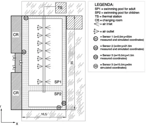
5.1 Fidia swimming pool layout . . . 35

5.2 Sensor network configuration inside Fidia swimming pool space 36 5.3 Air temperature trends in Fidia indoor swimming pool . . . 36

5.4 Quality indexes of the measurement (left figure) and simulated (right figure) solutions . . . 37

5.5 Optimal sensors location retrieved with simulated and measured datasets of temperature . . . 39

5.6 Simulated (left side) and Measured (right side) air Temperature trend along the perimeter . . . 40

5.7 Difference between simulated and measured temperature gradi-ents along the perimeter of the swimming pool . . . 41

5.8 Comparison between the old thermostat and the new optimal bias due to sensor placement for temperature monitoring . . . . 42

5.9 Fitness room plant and ventilation system design . . . 42

5.10 Sensor network placement for the fitness room . . . 43

5.11 Air temperature distribution inside the fitness room . . . 43

5.12 Coordinates of installation of optimal sensor position for the fitness room . . . 45 5.13 Trade-off between energy consumption deviation and number of

(11)

List of Figures

5.15 Sensor network design of open space office, Engineer Building NUI Galway) . . . 49 5.16 Temperature trends inside the open space office during one day,

Engineer Building NUI Galway . . . 50 5.17 Temperature deviance between reference temperature and

opti-mal solution during one day, inside the open space office of the Engineer Building NUI Galway . . . 51

(12)

List of Tables

1.1 Literature review key features . . . 3

3.1 Thermal model parameters . . . 18

4.1 tab:Optimization stages requirements and outputs . . . 25

4.2 Ranking deviances assignment process . . . 28

4.3 Classification criteria of the cross-validation process . . . 32

4.4 Example of classification process . . . 33

5.1 Comparison of the statistical features between the measured and simulated optimal solutions . . . 38

5.2 Comparison of the statistical features between the measured and simulated optimal solutions . . . 40

5.3 Statistical features of the solution 1 sensor for the fitness room 44 5.4 Statistical features of the solution 2 sensors for the open space office . . . 50

(13)

Chapter 1 Introduction

1.1 Background and motivation

Monitoring spatial phenomena as indoor air temperature is a challenging task, especially when applied to large indoor spaces. Large spaces include indoor sport spaces, open space office, entertainment buildings, cruise ship, aeroplane, where the air temperature is not homogeneously distributed, so the monitored values can be different from point to point at a given instant. In particular, phenomena as air stratification and stagnation may be present, causing sig-nificant horizontal and vertical temperature gradients [1]. This phenomena are generally due to large floor area, high height, high percentage of glazing surfaces, incoming direct solar radiation, errors on ventilation system design and heating/cooling sources randomly distributed in the space. The indoor thermal condition are normally monitored using traditional methods as single point temperature sensors, usually located in the return duct of the ventilation system or in a single point of the space, without taking into account air temper-ature gradients that could occur in the occupied space. Additionally, common practise is to design a monitoring system using criteria based on experience. So, conventional air temperature monitoring techniques could reach a level of measurement uncertainty that prevent accurate thermal comfort evaluation [2, 3] and effective climate control strategies operated by the HVAC (Heating, Ventilating and Air Conditioning) system [4, 5, 6]. Considering that measuring the air temperature inside critical environments, such as large spaces, using a limited number of sensors, is a challenging task to achieve; so the decision mak-ing process leadmak-ing to selection of sensors number and placement is challengmak-ing too. Considering what said above, a dedicated methodology focused on sensor network design optimization, in terms of sensors number and locations, taking into account the impact on thermal comfort and HVAC operation, deserves to be investigated.

(14)

Chapter 1 Introduction

1.2 Current approach

Different methodologies have been developed to achieve the indoor air tem-perature monitoring optimization. For instance, [7] developed and applied a methodology coupling CFD (computational fluid dynamics) and GA (Genetic algorithm) to define the optimal placement of temperature sensors in a single zone. [8] proposes a strategy for using wireless sensor network to monitor the temperature distribution in a large-scale indoor space, improving the quality of the measurements, identifying the temperature distribution pattern of the large-scale space, and optimizing the allocation of multiple supply air terminals. [9] uses a CFD calibrated model to generate a reduced order model to reproduce the indoor air dynamics allowing the rooftop units (RTs) assessment.[10] pro-poses a CFD-BES co-simulation strategy through indoor temperature sensor placement optimization linked with HVAC energy consumption and thermal comfort. The paper [11] proposes a CFD based supervisory demand-based temperature control applied to large-scale room to improve HVAC control and energy performances. In [12], a methodology based on CFD model was de-veloped for sensor placement optimization on a Greenhouse environment. [13] proposes a CFD model approach for optimal wireless sensor nodes installa-tion in large-scale room. [14] presented a “quasi-3D” modelling approach for thermo-hydraulic simulation of airflows and used it to investigate heaters and sensors positioning issues in a room. [15] proposes an ESP-r model approach to investigate the influence of temperature sensor placement on the heating energy consumption and thermal comfort. While, [16] developed a dedicated zonal model to study the influence of the sensor positioning in building ther-mal control. [17] proposed a zonal model to investigate the applicability of a new approach designed for prediction of energy consumption of a residential building, equipped with and underfloor air distribution system (UFAD). On the contrary, [18] proposed a data-driven approach to model the thermal dynamic of a large space through a combination of data clustering and system identifi-cation techniques. This approach attempts to reproduce the dynamics of the environment in a very accurate way and requires a fine-grained instrumenta-tion measuring for a long period. The data mining procedure is also applied in [19] to analyse off-line dataset and investigate the distributions of indoor air temperature, humidity and lighting in an indoor environment. [20] presented a method that provides analysis of measured data to reduce the number of sensor nodes deployed while preserving the quality of the information. Tab. 1.1 sum-marizes key features as measurement approach for thermal characterization of the space, methodology for the dataset generation, optimization strategy and objective for the proposed studies.

(15)

Table 1.1: Literature review key features

Ref. Space Measurement Dataset Optimization Objective [7] Small Spatial air

temper-ature distribution

CFD Balance between measurement accuracy and in-frastructure costs

Optimal air tempera-ture monitoring based on measured data and CFD model.

[8] Large Horizontal air tem-perature distribu-tion

CFD Optimizes the sup-ply air flow rate al-location according to temperature dis-tribution pattern

Optimal supply air flow rate allocation.

[9] Large RTUs supply and return air temper-atures, external temperature

CFD Sensor retrofit analysis

Sensor retrofit analy-sis linked with thermal comfort and RTUs en-ergy usage.

[10] Small No measurement CFD Sensor retrofit analysis

Sensor retrofit analy-sis linked with thermal comfort and HVAC en-ergy usage.

[11] Large Sensor network at breathing level

CFD Optimal HVAC

control strategies

Thermal comfort and HVAC energy usage.

CFD Optimal sensor placement

Optimal temperature monitoring and model calibration.

CFD Optimal sensor placement

Optimal temperature monitoring and model calibration and HVAC control.

[14] Small 3D air temperature distribution from MINIBAT test cell experiment and simulation

Zonal model

Sensor position retrofit linked with heating control system

Optimal sensor po-sitioning linked with optimal room heating control and model calibration.

[15] Small Meteo station and indoor air temper-ature

ESP-r Sensor position retrofit linked with heating control system

Impact of sensor place-ment on the heating thermal consumption and thermal comfort.

[16] Small Air temperature vertical gradient

Zonal model

Vertical tempera-ture monitoring

Impact of sensor place-ment on vertical tem-perature gradient.

[17] Small Air temperature vertical stratifica-tion Zonal model Vertical tempera-ture monitoring

Prediction building en-ergy demand.

[18] Large Spatial thermal distribution, rate airflow blown from the HVAC, occu-pancy detection Dynamic data-driven model Model develop-ment, validation and sensor cluster-ing

Optimization of the HVAC control based on sensor clustering and dynamic data-driven simulation model.

(16)

Ref. Space Measurement Dataset Optimization Impact [19] Large Horizontal air

tem-perature distribu-tion, relative hu-midity, light level

Data driven

Data mining to un-derstand distribu-tion of environmen-tal parameters

Development of methodology to pre-dict temperature map of the space.

[20] Small Spatial air temper-ature distribution, humidity and light level

Data driven

Sensors reduction Development of a methodology based on sensor clustering to reduce the number of sensor nodes.

According to the studies reported in Tab. 1.1 and the features of large spaces, the following outcomes are pinpointed:

• the horizontal air temperature distribution is one of the main physical property to be identified for climate characterization of a controlled large space;

• HVAC layout, user profiling, outdoor conditions (e.g. solar radiation magnitude and direction, neighbouring buildings, shadowing elements and seasonal climate variation) are the key factors to characterize, in both dynamic and static manner, allowing simulation or data driven ap-proach to capture the thermal behaviour of a controlled space;

• indoor spaces are typically controlled by HVAC systems, by means of a feedback loop, through a single point temperature sensor placed along the perimeter of the space or on the return duct;

• a widespread of temperature sensors is usually deployed for thermal char-acterization of large spaces, considering layout barriers for sensor place-ment, particularly in this type of environment;

• a review on the founded algorithms, solving the sensors placement op-timization issue, related to optimal temperature monitoring, highlighted that a unique recognised criteria is missing.

Considering the Tab. 1.1 and the outcomes, reported above, a CFD model [7, 8, 9, 10, 11, 12, 13] “provides far more accuracy, but has at least two draw-backs. The first and obvious one is complexity. The second is that it is not immediate to separate the (partial) differential equations that hold within a volume from the boundary conditions. The creation of modular models is thus a complex task, in some cases unavoidably leading to quite cumbersome soft-ware implementation. There exist CFD tools applied to buildings, e.g., Fluent [21], but they are mostly used for steady-state computations, and hardly ever considered in system-level stud” as outlined in [14]. In fact, a CFD model

(17)

problem definition, computational effort and time consuming processing, make it not suitable for the implementation and design within a general building sim-ulation program and control technology field. Moreover, the changes of interior layout and continuous fluxes of occupants during a day, typical of large spaces, can have a strong impact on the reliability of the CFD model. To overcome these issues, the studies [14, 15, 16, 17] developed a methodology based on both zonal model and measurements to calibrate and validate the simulation model, making it able to optimize the climate control of the space through optimal sensor deployment. The proposed zonal models need less computa-tional requirements compared with the CFD model, providing optimal results in terms of prediction of the air temperature distribution. On the other hand, they were developed to be applied on specific domains, making them limited for large space studies with such a specific thermal behaviour. The methodologies proposed in [18, 19, 20], basing on data driven approach, reproduce accurately the indoor thermal behaviour of the space, but they require a fine-grained in-strumentation measuring for long period. This aspect makes such approach difficult to apply inside large spaces, taking into account the use and layout of it, which are barriers for sensors deployment.

1.3 Proposed solution

Given the literature analysis illustrated in the previous section, this thesis in-vestigates and demonstrates a methodology for optimal sensor placement based two main stages: thermal characterization of the space and sensor network op-timization. The climate characterization of the environment is based on the sub-zonal breakdown of a large space. The entire volume is horizontally divided in a sub-volumes, aiming to simulate or measure the hourly temperature trends in each of them. Different approaches are allowed as simulation modelling or field sensors for restrict data-driven or a combination of the previous two, in or-der to obtain a calibrated sub-zonal model of the space. An upgraded version of a well-mixed multi-zone modelling tool, known as HAMBase [22] was developed to permit the simulation based approach. In case of data driven approach, the deployment of the sensors has to characterize the horizontal air temperature distribution of the space to identify its main climate characteristic, allowing sensor placement optimization. A third approach, based on sub-zonal model calibration, was developed to generate high quality temperature distributions improving the accuracy of the optimization outcomes. The goal of the pro-posed methodologies for climate characterization of the space is to provide an intermediate approach, which reduces complexity and costs included on CFD, avoids the extensive sensors deployment and cost found on the data driven ap-proaches and can take advantages from the zonal model approach.

(18)

Regarding the second stage, optimization, looking the outcomes form the anal-ysis on the proposed state of the art, it should be underlined that a sensor network can be optimized using different criteria depending on the final goal of each proposed methodology, highlighting the lack of a unique recognised crite-ria. The final goal of this study was to develop a methodology to optimize the design of a sensor network for indoor air temperature monitoring though holis-tic criteria, which are based on the minimum sensors number that minimizes the measurement uncertainty, evaluating its impact on the indoor thermal comfort and operation costs (energy consumptions due to HVAC operation and cost of use of additional sensors). The developed methodology includes the application of a novel approach based on a measurement performance index, sum of statis-tical features, applied to the measurement deviation due to sensor placement. This approach can be considered unique, compared with the studies reported in Tab. 1.1, as it is focused on improving the measurement accuracy linked with positions and number of sensors. The optimization continues performing a sensitivity analysis evaluating the impact of the measurement uncertainty of the indoor air temperature, due to sensors position, on the indoor comfort level and energy consumption due to HVAC operation. The objective is to provide a methodology modular, able to cover most of the solution founded in the state of art, providing novelty trough the measurement performance index development.

1.4 Thesis outlines

The work presented in this thesis was firstly launched in [23], where a first step of the current methodology was made and included on a tool prototype called Sensor Optimization Unit (SOU). This tool was based on a user interface for data input, thermodynamic simulation of the space and a Genetic Algorithm as core of the optimization process. This thesis presents the development of an updated version of the SOU, the current methodology used the previous one as base. The work done in this thesis and in [23] is part of the FP7 EU project SportE2 [24] that developed a scalable and modular BMS (Building Management System) dedicated to sports and recreational buildings. Sport facilities are unique by their physical nature, energy consumption profiles, the usage patterns of people inside, ownership, and comfort requirements, so a ded-icated BMS is needed. SportE2 _{BMS includes four modules providing smart}

metering, integrated control, optimal decision-making and multi-facility man-agement. The smart metering system objectives are to monitor the energy performance of the whole building [25] and to characterize the building

(19)

ser-Chapter 1 Introduction

large spaces to optimize the indoor air temperature monitoring. The increased accuracy on the temperature data were used by control and optimization mod-ules to increase the facility efficiency in terms of thermal comfort and energy consumption. Three different papers are then reported, which were published during the project, to underline the importance of air temperature accuracy on developing optimal HVAC control strategies. The work proposed in [26] showed how the SportE2 optimization system can support building managers in implementing energy efficient optimization plans. The study reported in [27] proved that the same optimization system was able to both predict and optimize energy consumption and thermal comfort inside an indoor swimming pool. The proposed study showed as an ANN (Artificial Neural Network) was used to run in near-real time an optimization algorithm to provide optimal HVAC set-points to maximize indoor thermal comfort with the minimum en-ergy consumption. It should be underlined that the environmental conditions were retrieved from a sensor network installed in a swimming pool and the SOU was used to optimize its design, in order to increase the measurement accuracy of the air temperature, which was a key parameter to calculate a calibrated thermal comfort index used by the optimization module. Considering that the air temperature is one of the most influential variable on the comfort evalu-ation inside sports environments [2] and considering the state of art reported in the previous paragraphs, the level of accuracy of the air temperature mea-surement is a crucial task to address, in order to achieve fine climate control operated by HVAC systems, leading to objectives such as energy efficiency and maximization of the comfort level, as done by the BMS developed in SportE2_.

Taking into account the outcomes reported previously, the importance of the measurement accuracy on the environmental climate control chain was proved. Thus, a dedicated methodology is needed to investigate how the sensor network design can be optimized to achieve the maximum measurement accuracy with the minimum number of sensors deployed, evaluating the impact on thermal comfort and HVAC energy consumption.

This thesis presents the development, application and validation in real cases studies of the developed methodology to address that issue. The finalization of the study, presented in this thesis, was performed during a six months re-search experience with the IRUSE (Informatics Rere-search Unit For Sustainable Engineering) research group in Galway, Ireland, from April 2015 to September 2015. The hosting building of the faculty was the Engineering Building NUI Galway, which is equipped with a BMS and an extensive set of sensors captur-ing environmental, energy and structural characteristics of the buildcaptur-ing. Air temperature data, gathered from sensors installed inside an open space office of the Engineer Building, were used as test case for the SOU optimization al-gorithm application.

(20)

The entire methodology is described starting from Chapter 2, where the ap-proach is summarized in total and the main characteristics are underlined in order to clarify the proposed solution for the optimal sensor placement. Chap-ter 3 presents the thermal characChap-terization of the space; in particular the section describes the approaches allowed by this methodology for the dataset genera-tion process. Chapter 4 contains the descripgenera-tion of the optimizagenera-tion process used to optimize the sensor network design. The application and validation of the entire methodology is performed in three different test cases and it is fully described in Chapter 5.

(21)

Chapter 2 General approach and methodology

applied

This thesis proposes a methodology based on a novel measurement performance index to optimize the temperature monitoring in large spaces. The final out-come is the optimal number of the sensors and installation coordinates inside the environment. The entire methodology can be divided in two main steps:

1. An approach based on simulation, measurement or hybrid, generates a dataset representing the horizontal air temperature distribution inside the space; the previous chapter identified it as the key climate condition from large spaces, which needs to be captured for the optimization task; 2. An optimization solver uses the dataset generated in step 1 to optimize the sensor network design, in terms of number of sensors and placement along the perimeter of the space under study; the optimization first evalu-ates the measurement accuracy due to sensor position and then its impact on thermal comfort and HVAC operational cost.

The first one is described in Fig. 2.1 and it can be approached through three different ways: simulation, measurement or hybrid, a simulation model cali-brated with measurements. The simulation approach is based on a sub-zonal model of the space, which divides the entire volume horizontally in equals sub-volumes, where the air can be considered perfectly mixed. A dedicated graphical user interface (GUI) was developed to guide the user through the data implementation process for the building, in order to run the simulation. Once the GUI (Appendix A) is filled, the software starts to build the sub-zonal model of the space and automatically calculates the needed number and po-sitions of sub-zones. The process depends on numerical requirements, which are defined by the solver behind the simulation. The simulation outputs are hourly temperature trends for each sub-volume reaching a maximum period of one year. These time series represent the temperature values of each central node of each air sub-volume, considered perfectly mixed. The data-set gen-eration based on measurement requires the installation of a temporary sensor

(22)

Chapter 2 General approach and methodology applied Feasibility analysis Selection of one of the proposed approaches Sub-zonal model Sensor network deployment Interpolation function Measurement Simulation Sub-zones temperatures trends Facility audit for data input

Facility audit for data input & dedicated sensor network deployment Simulation model calibration Sub-zonal calibrated model

Figure 2.1: Dataset genaration approaches allowed by the SOU

network. First the space is virtually divided in sub-volumes, which are hori-zontally distributed in equal manner. The deployment process of the sensors has to guarantee that each sub-volume holds at least one temperature sensor; the number of nodes to be installed in each sub-volumes depends also on their dimension, taking into account that the sensors have to be deployed along the perimeter (due to large space layout constrains). As for the previous approach, the objective is to obtain temperature trends on the central points of the vir-tual sub-volumes; so a dedicated interpolation function, based on the weighted inverse distance method, was developed to obtain the final dataset useful for the optimization process. In case of simulation model calibration, a facility audit allows to collect data generating a sub-zonal model of the space following the approach presented above and a sensor network installation is mandatory as well; the selected measurement equipment should be deployed to capture the indoor thermal condition, but additional sensors need to be installed outdoor, in order to monitor the external climate conditions. This third approach is a combination of the previous two. A dedicated calibration process was de-veloped to generate high quality indoor air temperature trends allowing most accurate optimization of sensor network design.

(23)

Chapter 2 General approach and methodology applied

just on measurement performance criteria. The second one (Fig. 2.3) generates

Sub-zones temperatures trends Measurement performance index Measurement performance criteria satisfied? Yes Sensor positioning algorithm Plant with positioned sensors No Best solutions: 1 sub-zone to N-1 sub-zones

Solution 1 sub-zone Best solution with +1 sub-zone Best sub-zone/ subzones for sensor positioning Interpolation function Temperature trends along the perimeter From dataset generation

Figure 2.2: Optimization workflow based on measurement performance index a trade-off between measurement accuracy (number fo sensors), taken from the previous step, and impacts on indoor thermal comfort and energy consumption due to HVAC operation. In both optimization procedures, the provided output is the space plant with the sensors nodes placed in optimal perimeter locations. The first step of optimization takes the simulated or measured temperatures trends coming from the sub-volumes dividing the space (Fig. 2.4). Thus, the mean of these trends is calculated and defined as reference temperature, which is referred as the best accuracy available for the air temperature monitoring inside the entire air volume, considered as perfectly mixed. The objective of the optimization is to define the minimum sensors number to achieve the mini-mum deviation from the reference temperature. As next step, the optimization

(24)

Chapter 2 General approach and methodology applied Sub-zones temperatures trends Measurement performance index Sensor positioning algorithm Plant with positioned sensors Best solutions: 1 sub-zone to N-1 sub-zones Interpolation function Temperature trends along the perimeter Facility audit for data input Single zone model Measurement deviations Sensitivity analysis PMV and energy consumption deviations Best sub-zone/ subzones for sensor positioning From dataset generation

Figure 2.3: Optimization workflow based on trade-off between number of sen-sors, thermal comfort and HVAC energy consumption deviations

(25)

solver calculates the mean temperature trends by combining all the sub-zones trends, retrieved from the dataset generated from the previous step. The

op-Figure 2.4: From zonal model to sub-zonal model

timization process continues calculating the deviances between the reference temperature trend and each trend obtained as combination between sub-zones. The deviances trends represent the measurement bias due to sub-zones selec-tion to solve the temperature monitoring issue. Each deviance is assigned to the sub-zones selected as possible optimal solution. The optimization process proceeds applying a measurement performance index to each deviance trend. This index is made of a sum of statistical feature, which is the key novelty of the proposed approach. Specifically, each statistical feature evaluates the measurement error in terms of:

• Mean deviation, referred as the tendency to over/under estimate the aver-age temperature of the entire space. An absolute low value of mean devia-tion prevents waste of energy and discomfort brought by overheating/over-cooling;

• Standard Deviation, which represents the final measurement uncertainty. This feature is fundamental for thermal comfort evaluation and optimal HVAC system regulation;

• Outliers, defined as the amount of time spent by the monitoring system measuring outside the sensor uncertainty value, which is usually provided by the manufacturer;

• Z test, quantifying the effect of external perturbations on the measure. Once the performance index is calculated for each deviance, it represents a quality index for each combination of sub-zones selected as potential optimal solution for sensor deployment. The solutions (deviances) are ranked basing on the index values calculated in the previous step. The first optimization

(26)

step’s objective is to select the optimal sub-zones where the sensor should be installed, in order to provide the required measurement performance, estab-lished by pre-defined criteria. The final position of installation for the sensor inside each sub-zone, selected as optimal, is then provided through the applica-tion of a dedicated posiapplica-tioning algorithm. A deeper analysis is done trough the second step of optimization. It proceeds generating a single zone model of the space, which outputs hourly values of predictive mean vote (PMV) and energy consumption due to heating/cooling system covering a maximum period of one year. The deviances, retrieved from the previous optimization step due to the different optimal sub-zones configurations, were used to perform a sensitivity analysis on the single zone model to evaluate the impact of measurement ac-curacy (number of sensors) on both indoor thermal comfort level and energy consumption. The optimization process was divided in two steps, aiming to al-low a modular approach for the sensor optimization task depending on the user needs and cost constraint. In fact, the second stage of optimization needs the development of an additional simulation model of the space and a sensitivity analysis based on calibrated algorithms.

(27)

Chapter 3 Dataset generation

3.1 General approach

In the previous chapter the objective, the needed inputs, the optimization ap-proaches of the SOU were introduced to show a general picture of the software. This chapter will describe in details the approaches allowed by the SOU for the dataset generation. The objective is to generate the necessary datasets used as inputs by the optimization algorithms of the SOU to calculate the optimal de-sign of the sensor network in terms of minimum number of sensors and relative placement.

3.2 Simulation

The objective is to have a simulation model able to characterize the indoor horizontal air temperature distribution of a large space at a certain heigh level (typical height of installation for a thermostat). The thermal behaviour of large spaces is highly influenced by external and internal factors. External factors are the outdoor weather conditions, as direct and diffuse solar radiation, external air temperature and relative humidity, wind direction and velocity, influence of adjacent rooms, external shadowing elements. Otherwise, thermal properties of the envelope, glazing surfaces properties, building orientation, use profile of the space, spatial and temporal characterization of the internal loads, charac-terization of local HVAC, primary systems and control strategies are the main indoor factors influencing the indoor air temperature distribution. A thermal modelling aiming to relate the space heat, air and moisture influence on the temperature distribution has to include the possibility to simulate the factors mentioned above.

A dedicated thermal modelling was developed for the discretization of the hor-izontal air distribution of the space, simulating a dataset of the temperature distributions. The thermal model is based on the HAMBase library, that is an open library implemented in Matlab computing environment [28], which

(28)

Chapter 3 Dataset generation

is useful for code customization purpose. It simulates the hourly indoor air temperature and humidity of a multi–zone building with a relatively small mathematical computational requirement. De Wit described extensively the physics of this model in [22].

The multi-zone model approach of the HAMBase is not accurate enough to simulate the temperature distribution of a large space in a building, because this approach calculates one air temperature value per hour that represents the average temperature value inside the whole space; in fact, the HAMBase does not allow the spatial discretization of the mentioned factors influencing the horizontal temperature distribution. The sub-zonal approach can overcome the lack of resolution of the multi-zone approach. The HAMBase library was then customized to develop a sub-zonal model from the multi-zone one. The updated version of the multi-zone model divides the space, which would nor-mally be a single zone, into a coarse network of smaller sub-zones, as shown in Fig. 2.4. Each sub-zone has to satisfy the hygro-thermal and the inter-zonal airflow models, then the air contained inside each sub-zone, dividing the single zone, is assumed to be perfectly mixed. The sub-zonal approach permits to increase the resolution of the air temperature distribution on a virtual horizon-tal plane of the space. The updated model is able to generate the dataset of temperatures requested by the optimization solver.

The new sub-zonal model represents the sensor network and simulates the value of air temperature of each sub-zone covering a period of one year with a fixed time step. The simplified approach of the proposed tool allows the problem set-up with low computational load for a user that has no specific technical expertise (as required for a CFD). It also allows to simulate the thermal be-haviour of an environment during one-year period, taking into account the environment weekly use profile, the influence of adjacent rooms, internal loads distribution in space and time, external weather conditions and external shad-owing elements, that impact significantly on the temperature distribution. Since that the developed thermal model is a modified version of HAMBase, several parameters were added to the ones already needed by the original tool and the existent documentation is not enough to run the simulation. Moreover the tool presented in this thesis is meant to be used by HVAC engineer, who are not simulation expert, so a dedicated (GUI) was developed guiding the end-user from the dataset generation process to the optimization goal. It contains the total amount of the necessary inputs to run the simulation plus optimiza-tion process. The basic idea behind the GUI is to make the tool user-friendly, so a certain amount of parameters are automatically derived and implemented during the GUI filling phase.

(29)

3.3 Measurement

The data driven approach is based on field measurement coupled with an in-terpolation algorithm. The entire volume of the space is virtually divided in horizontal sub-volumes, equally distributed in the space. The virtual division follows the one generated by the sub-zonal approach. Then, at least one sensor has be installed inside each sub-volume, acquiring temperature data for a cer-tain period, sufficient to capture the typical usage profile. The sensors should be installed at typical thermostat height above the floor, along the space perimeter and near the occupied zone. It is fundamental to collect information about the room usage, which has a strong influence on the indoor temperature distribu-tion. Finally, the gathered data are processed by an interpolation algorithm to generate temperature trends that correspond to the value of the temperature in the central point of the virtual sub-volume, dividing the entire space. The sensors should not be installed where:

• there are unusual heating conditions, such as: direct sunlight, near lamps, radio, TV screens, near hot water pipes in a wall;

• there are unusual cooling conditions, such as: in a draft from a stairwell, door, or window;

• air circulation is poor, such as: in a corner, an alcove, behind an open door.

3.4 Simulation model calibration

Model calibration means a data-driven process that leads to the optimal values of the model parameters, allowing the model to simulate the output closest as possible to the measured one. The calibration activity can be manual by direct tuning the model parameters, until the comparison between output and measurements reach the desirable uncertainty. The developed methodology is a quasi-automated calibration procedure due to few operations that still need user interaction. The following list contains the requirements that were fulfilled to develop the model calibration process:

1. Selection of the model parameters that need to be calibrated;

2. Build a robust and effective optimization process able to find the best set of parameters values;

3. Dedicated measurement procedure to retrieve the needed data from the field, fundamental for the model calibration process.

(30)

3.4.1 Requirements for problem solving

The first step to build a robust calibration method was the selection of the most influencing input parameters for the model, which the calibration pro-cess should focus on. In [29] the effect of uncertainties of a selected group of the HAMbase input parameters were investigated and the simulation model resulted most sensitive to changes in insulation material layer thickness, venti-lation rate, and the internal surface heat transfer resistance.

Starting from that, the number of parameters under study was increased bas-ing on the experience and knowledge made durbas-ing the developbas-ing and usage phase of the thermal model. This process brought to a selection of a group of parameters reported in the following Tab. 3.1.

Parameter Short-Unit Range

Interzonal airflow Linkv [m3/s] ±20[%]

Casual heat gains Qint [W ] ±50[%]

Water vapour sources Gint [Kg/s] ±50[%]

Air changes Vmin [1/h] ±50[%]

U-value transparent surfaces Uglas[W/m2_K] _±20[%]

Solar gain factor ZTA[−] ±20[%]

Material layer thickness D [m] ±20[%]

Internal surface heat transfer resistance Ri [Km2/W ] ±20[%] Convection factor of the heating system CFh [−] ±20[%] Heating system time constant Tau [h] [0; 1]

Heating capacity P [W ] ±20[%]

Inlet factor If [−] [0; 1]

Solar factor Sf [−] [0; 1]

Table 3.1: Thermal model parameters

The range column of the Tab. 3.1 represents the upper and lower bounds of freedom for the parameters values. The bounds are expressed in percentage of the initial guess of the parameters, which represents the initial values of them considered as starting point for the optimization process. Some of the parameters (Tau, If, Sf) can just assume a value between zero and one. In case the room is still in design stage, some of these data can be extract from the project itself. In case of retrofitting of an existing room, the calculus and definition of them could be a challenge.

A dedicated audit procedure for the space has to be performed. The objec-tive of the audit is to obtain the necessary data to run the simulation model though geometrical characterization of the space, the identification of the

(31)

in-Chapter 3 Dataset generation

Tab. 3.1 are affected by high level of uncertainty, cause difficult to evaluate and measure. The calibration modelling process allows to evaluate them in a most accurate way. The selection of the range of freedom for the parame-ters is mostly based on the experience matured during the development and application phases of the thermal model.

3.4.2 Optimization process for calibration

A detailed review of methods to match building energy simulation models to measured data is reported in [30], the paper reports an overview of the cur-rent approaches for model development and calibration. In [30] an extended comparison between calibration modelling approaches for predicting building energy performance is reported. Kramer in [31] developed an optimization rou-tine to fit the output of simplified hygro-thermal building model in state space form of the HAMbase with measured data. The optimization process described in [31] was developed in Matlab, as the tool presented in this thesis, and it has been proved to be robust. Those conditions were considered sufficient to select the mentioned approach as base of the optimization process proposed in this thesis. The next paragraphs will describe how that methodology was modified to fulfil the goal of this study. Two solvers mainly compose the optimization process: the first one is based on Genetic Algorithm (GA) [32], the second one on Pattern Search (PS) method. In [31] the author underlined as “GA has proved to be a very promising in finding a near optimal solution in very big solution spaces”, so the first step of the optimization will provide a quick near optimal solution for the parameters. Therefore, the genetic approach is used. GA is one of the most powerful heuristic method to solve optimization problems [33]. In particular the algorithm used in this study, it is implemented inside the Matlab optimization toolbox by default and fully described in [34].

The optimization process is represented in Fig. 3.1, where it can be seen as the optimization process start from the definition of a first guess of parameters values and their upper/lower bounces. These parameters are the inputs for the thermal model that produce the first temperatures map. The fitness function evaluates the quality of the solution through comparison between measured and simulated data. If the quality of the solution is not enough, the optimiza-tion process continues through the genetic algorithm that produces another set of possible solution for the parameters. These solutions are sent to the thermal model, which produces outputs and the process iterates until the stop-ping criteria are satisfied: deviance between measured and simulated outputs equal to 0.1 or the number of iterations reached the maximum value of 100. The set of parameters that satisfied the stopping criteria is considered as the optimal set and the first stage of optimization can be considered concluded.

(32)

Chapter 3 Dataset generation First parameters guess Stopping criteria satisfied ? Optimal parameters (GA) Fitness function Thermal model Genetic algorithm NO New set of parameters YES

Figure 3.1: First optimization stage using Genetic Algorithm

The second stage is based on the pattern-search algorithm, also implemented inside the Matlab optimization toolbox [34]. As reported in [31],”the Pattern Search algorithm is a gradient free, deterministic algorithm, very suitable for not smooth and discontinuous problems”.

Optimal parameters (GA) Stopping criteria satisfied ? Optimal parameters Fitness function Thermal model Pattern search NO New set of parameters YES

(33)

Starting for the solution provided by the GA on the first stage, the PS [34] polls solution points around the starting one, the solution that improves the fitness function becomes the new starting point. The process continues until the stopping criteria are reached: solution accuracy equal to 0.1 or maximum number of iterations equal to 1000. The Pattern-search algorithm defines the global solution, in other words the final values of the parameters (Fig. 3.2). Others optimization algorithms as multi-starting point, particle swarm opti-mization were taken into account. The selection of the described workflow was made based on comparison of performances with them, in terms of quality of fitness function evaluation and time-consuming point of view.

3.4.3 Fitness function

In general, an optimization process needs the design of a dedicated fitness function. Given a particular solution (set of parameters), the fitness function returns a single numerical value, or "figure of merit", which is supposed to be proportional to the "utility" or "ability" of the solution. The objective of the optimization is to provide a set of parameter able to reproduce the maps of the air temperature distribution in the space, for the point of view of absolute temperature values inside the sub-zones and temperature gradients between them. Where the sub-zone is represented as one temperature node in the centre of the volume, considered as well mixed. The fitness function takes as inputs the measured (Eq. 3.1) and simulated (Eq. 3.2) temperatures expressed as following: Tm= ⏐ ⏐ ⏐ ⏐ ⏐ ⏐ ⏐ ⏐ Tm1,1 . . . Tm1,N .. . . .. ... TmH,1 . . . TmH,N ⏐ ⏐ ⏐ ⏐ ⏐ ⏐ ⏐ ⏐ (3.1) Ts= ⏐ ⏐ ⏐ ⏐ ⏐ ⏐ ⏐ ⏐ Ts1,1 . . . Ts1,N .. . . .. ... TsH,1 . . . TsH,N ⏐ ⏐ ⏐ ⏐ ⏐ ⏐ ⏐ ⏐ (3.2)

Where N represents the number of sub-zones (matrix columns) and H the num-ber of hours (matrix rows) for a maximum of 8760 (one year). First the fitness function calculates the deviances between measured and simulated tempera-tures for each sub-zone as following (Eq. 3.3):

∆1,1= Tm(1↦→H,1)− Ts(1↦→H,1) .. . ∆N,N = Tm(1↦→H,1)− Ts(1↦→H,1)

(34)

Then calculates the temperature gradients between each possible sub-zones couples for the measured (Eq. 3.4) and simulated ones (Eq. 3.5) in a separated way as following: ∆m(1,2)= Tm(1↦→H,1)− Tm(1↦→H,2) .. . ∆m(N −1,N )= Tm(1↦→H,N −1)− Tm(1↦→H,N ) (3.4) ∆s(1,2) = Ts(1↦→H,1)− Ts(1↦→H,2) .. . ∆s(N −1,N )= Ts(1↦→H,N −1)− Ts(1↦→H,N ) (3.5)

The next step is the calculus of the deviances between measured (Eq. 3.4) and simulated (Eq. 3.5) gradients as following (Eq. 3.6):

∆1,2= ∆m(1,2)− ∆s(1,2) .. . ∆N −1,N = ∆m(N −1,N )− ∆s(N −1,N )

(3.6)

Then the fitness function apply the Root Main Square Error (RM SE) operator to each delta calculated previously as following (Eq. 3.7):

RM SE1,1 = √ 1 n ∑ ∆2 1,1 .. . RM SEN,N = √ 1 n ∑ ∆2 2,2 .. . RM SE1,2 = √ 1 n ∑ ∆2 1,2 .. . RM SEN −1,N = √ 1 n ∑ ∆2 N −1,N (3.7)

(35)

The goodness of each solution is given by the minimization of the following equation (Eq. 3.8): F itness = w1∗ ( 1 n ∑ (RM SE1,1+ . . . + RM SEN,N) + w2∗ ( 1 n ∑ (RM SE1,2+ . . . + RM SEN −1,N) (3.8) Where w1 and w2 are weighted factors useful to customize the optimization process. The first term of the equation represents the deviance between mea-sured and simulated temperatures relative to the same sub-zones. The second term represents the deviance between measured and simulated temperatures, calculated as gradients between different sub-zones. The different algorithms run minimizing this function and the process continues until stopping criteria are reached. The criteria are two, the first is called stall, when the fitness func-tion values is less than funcfunc-tion tolerance (1e-1); while the second one appears when the algorithm reach a pre-defined maximum number of iterations (100 in case if GA and 1000 in case of PS).

3.4.4 Measurement data for model calibration

The necessary condition of a calibration modelling process is the knowledge of the output and modelling the physics of the system under study in the most accurate way. In this case, the output are measured data, which represent the indoor air temperatures values for the different sub-zones, which it has been divided the space. While, to model the indoor environmental conditions in a correct way, accurate data regarding the outdoor conditions are mandatory. The simulation uses as external inputs a meteofile of hourly weather data in-cluding some data of the location as latitude, longitude, time zone and albedo of the site. The file must start at 1 January and should have at maximum 365 days. A longer period than 365 days can be simulated but then the year is repeated. In leap years the last day is used twice. The meteofile contains parameters as year, diffuse solar radiation, 10*exterior air temperature, Direct solar radiation (plane normal to the direction), cloud cover(1...8), 100*relative humidity outside, 10*wind velocity, wind direction. Then hourly meteofiles of an average year can be generated with the program METEONORM [35]. The meteo file data can be downloaded using the SOU user interface through the website [36]. To build an effective calibration method the external conditions should correspond to the real measured one inside the space, during the same monitoring period. Since that the data about the indoor temperature distri-bution can be retrieved installing the sensor nodes inside the space to be used as output, external sensors are also requested. So, the installation of a meteo station outside the facility is recommended, but it can be not cost effective

(36)

for sensor network optimization purpose. The idea is to install sensors for air temperature and relative humidity external monitoring and then ,since that, the direct and diffuse solar radiation is one of the most influential external parameter, in case the data is not available, it can be retrieved with a suf-ficient accuracy using a methodology fully described in [37]. The developed algorithm was implemented in this study, allowing to calculate the diffusive and direct solar radiation from external air temperature and relative humidity trends. The time window of measurement campaign should be enough to cover the seasonal thermal characterization of the environment; the acquisition rate should be equal to a minimum value that allows a correct digitalization of the phenomena under study.

3.4.5 Sub-zonal model calibration

The indoor temperatures, available from the installation of the sensor network, are gathered into daily groups, maintaining hourly sampling. The groups are further filtered keeping just hourly temperature profiles during the HVAC op-erational hours. The filtered data are processed by cross-correlation selection criteria. The output of the selection process has to lead to a minimum number of 10 folds [41] of daily trends that reported mutually high correlation values. This sub-group of the initial one represents the indoor thermal behaviour for the room. The selected data are divided in 10 folds for further analysis us-ing a cross-validation method, but for the model calibration process the entire amount of selected data is used.

In the meanwhile, a detailed facility audit allows the generation of a basic sub-zonal model. Then, the filtered data and the basic simulation model become the fundamental part of the model calibration process. The process of model calibration starts working iteratively through the optimization algorithms and the fitness function, deeply described in previous sections. The fitness function evaluates the quality of parameters using simulation and all the filtered data from measurement. The calibration drives to the definition of optimal values of thermal model parameters. The calibrated model is used to simulate the in-door air temperature inside each sub-zones dividing virtually the environment, during the period under study: one month, an entire season, a year, depending on the goal of the optimization.

(37)

Chapter 4 Optimization solver of the SOU

4.1 General approach

The workflow of the tool was presented in Fig. 2.1, 2.2, 2.3 and the previous chapters described the different approaches used to characterize the indoor envi-ronmental condition inside the space under study, generating hourly sub-zones air temperature trends. The optimization objective is to use these temperatures trends to design an optimal sensor network in terms of number of sensors and placement. The optimization task was divided in two steps to provide a most comprehensive supporting tool for HVAC engineer during the environmental monitoring design stage. In order to give a general picture of the different opti-mization stages, Tab. 4.1 summarized on the first three rows the requirements for each optimization stage based on the dataset generation approach, then the last row describes the different outcomes from each optimization stage.

Table 4.1: tab:Optimization stages requirements and outputs Measurement performance

evaluation

Sensitivity analisys Simulation Sub-zonal model 1- Single zone model

2- Sensitivity analysis Measurement Sensor network 1- Single zone model

2- Sensitivity analysis Calibrated

simulation

1- Sub-zonal model 2- Sensor network

1- Single zone model 2- Sensitivity analysis

Optimization output

Number of sensors and position base on measurement accuracy

Number of sensors and position based on measurement accuracy, impact on comfort and energy consumptions

(38)

Chapter 4 Optimization solver of the SOU

4.2 Measurement performance evaluation

The final optimization objective is the minimization of sensors number able to provide the minimum deviation from the measurement performed by refer-ence condition, at least one sensor in each sub-zone, which virtually divides the space. To this aim, the optimization solver receives the temperatures dataset, as shown in Fig. 2.2, evaluates the measurement performances of proposed sub-zones temperature trends combinations, in terms of numbers and positions against the reference temperature, which represents the uncertainty due to the sensors positioning and determines the optimal sub-zones for the sensors in-stallation.

The SOU thermal characterization provides indoor temperature trends used to define the maximum measurement accuracy achievable (reference condition), which is the temperature calculated as the mean value of the temperatures evaluated in the sub-zones. Then, the software calculates the deviation be-tween the reference temperature trend from the previous step and temperature trends derived by combinations of reduced sub-zones temperature trends. The optimization solver evaluates the measuring performance of each combination using a measurement performance index based on statistical features calculated on those deviations. In detail:

• The mean deviation that represents the distance from the reference con-dition; a mean value closer to zero corresponds to minor under or over esti-mation of the thermal conditions that could cause an overheating/overcooling or underheating/undercooling;

• The standard deviation, here considered with a coverage factor k=2, that is a measure of the deviation distribution around the mean value. Higher the standard deviation higher the uncertainty of the measurement; • The outliers period, expressed in hours, that is a measure of the

pe-riod where the standard deviation is higher than the sensor uncertainty (datasheet value), which is or will be installed to monitor the indoor temperature;

• The Z index, which represents the so-called z-statistic. It evaluates how close the deviation is to a Gaussian distribution. More Gaussian is the distribution, lower is the influence of perturbations on the measurement due to external factors.

Once that the performance index is calculated, a positioning algorithm defines the precise position of installation for each sensor node.

(39)

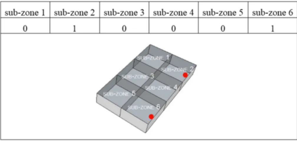
to 1 if the sensor is installed inside the sub-zone and 0 if not. Each sub-zones configuration can be represented as a row vector, so it is a sequence of bits (0 or 1) whose length is given by the number of sub-zones as shown in Fig. 4.1. The deterministic solver generates all the possible solutions of installation (a

Figure 4.1: Sensor network representation as bit string

string of bit for each one), that are 2n−1 _{combinations of 0 and 1, where n is} the total number of sub-zones. Then, the solver assigns a label to each row, represented by a number from 1 to 2n−1(set), which will be used to identified the configuration of the solution of installation, along the entire optimization process. Each sub-zones combination is compared to the reference condition (a string of ones), which is a temperature profile Tr calculated as the mean value of the n sub-zones temperature profiles (Eq. 4.1):

Tr= ∑n

i=0Ti

n (4.1)

The metric of comparison for each combination (set) is the deviation (Eset) with respect to Tr and calculated as following:

Eset= Tset− Tr (4.2)

Where Tsetis each temperature profile of the 2n−1, provided by the combina-tion of sub-zones and calculated as the mean value of the temperature profiles of each sub-zone included in the combination. Once calculated the deviations

Eset for all possible combinations, their statistical features, are evaluated. All the combinations are ranked (Tab. 4.2) according to each statistic and receive a score (Sz) equal to the position occupied in each ranking (R), in particular each

(40)

score is calculates as Sz(set) = (2n−1− R), where z = 1 to 4 and S1is the score

for the mean deviation, S2 for the standard deviation, S3 for the outliers and

S4 for the Z index. The sum of the scores, achieved in each ranking, provides

Table 4.2: Ranking deviances assignment process set Ranking (R) Mean deviation of each Eset

15 1◦ 0.1◦C

34 2◦ 0.14◦C

. . . .

2 2n−1 1 ◦C

set Ranking (R) Std deviation of each Eset

17 1◦ 0.13◦C

42 2◦ 0.25◦C

. . . .

1 2n−1 1 ◦C

set Ranking (R) Outliers of each Eset

14 1◦ 1

55 2◦ 3

. . . .

7 2n−1 681

set Ranking (R) Z index of each Eset

25 1◦ 0.7

36 2◦ 1.2

. . . .

2 2n−1 ₉

the performance index (Im) for all the monitoring configurations, calculated as following (Eq. 4.3):

Im(set) = S1(set) + S2(set) + S3(set) + S4(set) (4.3)

The output is a number 2n−1 of solutions with the respective performance index Im(set). Once that an Im is assigned to each combination of sub-zones (set), the algorithm groups the solutions in terms of sub-zones number and selects each solution that achieved the best Imin each group. The best sensors configuration, among the available, is the one that fulfils the defined criterion. The standard deviation, that represents the resulting measurement uncertainty due to sub-zones configuration, has to be lower or equal to the uncertainty of the sensor (from datasheet), which will be deployed or it is already installed in the sub-zone.

(41)

4.3 Sensitivity analysis

The first step of optimization calculates the best sensor network design in terms of number of sensors and position using a dedicated measured perfor-mance index, as explained in the previous section. A further investigation is needed to evaluate the impact of the measurement uncertainty on the indoor thermal comfort level and energy consumptions due to HVAC operation. This second step of optimization uses as inputs, from the previous step, the mean and standard deviations for each of the best sub-zones configurations based on the maximum Im. Then it generates a normal distribution for each of the re-trieved optimal sub-zones configurations. These normal distributions represent the measurement deviations for each solution from the reference condition. A single zone simulation model of the space has to be developed following the original simulation approach proposed by the HAMBase [22]. In case of ther-mal characterization of the space based on simulation approach or calibrated simulation approach, the needed parameters to build a single zone model can be retrieved from the sub-zonal one; while in case the dataset generation pro-cess is based on measurement, a dedicated facility audit has to be performed to obtain the needed parameters to build the single zone model.

The next step consists on the evaluation of the impact of the air temperature measurement deviations on comfort and energy efficiency, following the schema in Fig.4.2. Once that the single zone model is built, it produces as output

sin-‘ ‘ ‘ ‘ ‘ ‘

(42)

gle hourly air temperature trend, which represents the mean temperature of the entire air volume of the space, considered as perfectly mixed. The HVAC control system uses the hourly air temperature as feedback to carry out the thermal regulation of the space. The air temperature trend is used by the single zone model to calculate the PMV value though a dedicated algorithm described in [2]. The simulation model is also providing hourly energy consumptions due to HVAC operation. First, the single zone model simulates an ideal indoor temperature trend (Ta), considering the feedback value for the HVAC not af-fected by measurement deviation. Then it calculates the PMV value and the Energy consumption. The effect of the measurement deviation of the hourly air temperature trend (Ta’), due to the sensors positions, on the PMV’ and Energy consumption’ values is evaluated trough a Monte Carlo method. Following the [38], the number of sampling (Ta’) has to be equal to 106 _{expecting to deliver}

a 95% coverage interval for the output quantity. Where Ta’ is equal to Ta plus the measurement deviation evaluated for each optimized sensors configuration retrieved by the optimization algorithm and expressed as normal distribution. The propagation of the measurement uncertainty generates a deviation on the model outputs. The comparison between the outputs coming from the first ideal model and the outputs, coming from the perturbed one, is expressed on deviation respect the original values and plotted related the number of sensors of the different solutions. The analysis of variances drives the process to the selection of the best sensor configuration for the monitoring system.

4.4 Sensor positioning algorithm

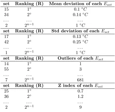
Once the sub-zones, where sensors should be installed, are identified by the first or second optimization methods, previously described, the precise location of installation for the sensor, inside the sub-zone, has to be delivered to the user. The nodal approach, adopted by the simulation model or measurement, considers the sub-zones as well mixed and the temperatures calculated are to be considered as the central temperatures in each sub-zone. An increase of spatial resolution is needed to define the deployment points for the sensors in the space. In fact, large spaces present constraints for network deployment and sensors cannot be placed in the centre, their deployment is usually restricted to the perimeter walls. The positioning algorithm provides the coordinates of installation of the sensor/sensors along the perimeter of the environment according to the sub-zones selected in the previous step. According to [39, 40], the perimeter temperatures values are calculated using an interpolation function based on the inverse distance weighting method [39] to obtain the

(43)

these source points are fixed as central node (Fig. 4.3) for each sub-zone that composes the entire space. The temperatures at the destination points (points marked in black, along the perimeter of the sub-zone, Fig. 4.3) are estimated by a linear combination of the values at the source points. The output is a map that represents the horizontal temperature distribution along the perimeter. Finally, the sensors positioning process selects for each sub-zone the perimetral

Figure 4.3: Sub-zone positioning algorithm

position that provides a temperature with the minimum root main square error (RMSE) with respect to the sub-zone central temperature.