Università Politecnica delle Marche
Scuola di Dottorato di Ricerca in Scienze dell’Ingegneria Corso di Dottorato in Ingegneria Civile, Ambientale, Edile e Architettura ---
The application of video-monitoring
data to understand coastal and
estuarine processes
Ph.D. Dissertation of:
Eleonora Perugini
Advisor:Prof. Maurizio Brocchini
Coadvisors:
Dr. Luciano Soldini Dr. Margaret L. Palmsten
Curriculum supervisor:
Prof. Stefano Lenci
Università Politecnica delle Marche
Dipartimento di Ingegneria Civile, Ambientale, Edile e Architettura (DICEA)
Acknowledgements
I would like to acknowledge my advisor Prof. M. Brocchini for coordinating my PhD study and for his availability and knowledge. I am especially grateful to my coadvisors Dr. L. Soldini and Dr. M. L. Palmsten for their patience, motivation and daily helps. Without their guidance and knowledge this work would not have been achieved.
I sincerely thank also A. Coluccelli for sharing the data of the COAWST Model, A. Sheremet for sharing measured spectra, P. Penna for sharing wave data of the Meda Station, C. Chickadel for sharing Matlab© codes, Carlo Lorenzoni for helping with the wave spectra analyses, B.G. Ruessink and T.D. Price for the information on the BLIM toolbox and R. Holman for his valuable suggestions on the cBathy. Special thanks go to J. Calantoni of the Naval Research Laboratory for his work of supervision of the EsCoSed project. The EsCoSed project was supported under base funding to the Naval Research Laboratory from the Office of Naval Research. Financial support from the ONR Global (UK), through the NICOP EsCoSed Research Grant (N62909-13-1-N020) is gratefully acknowledged.
Finally, I would like to thank my family: my grandparents, my parents, my brothers and all my dear relatives for believing in me and for supporting me in this important experience
Abstract
The present thesis details the first applications of a new video monitoring station, called SGS station, installed along the Adriatic coast, at the Senigallia harbour, Italy. SGS is not part of the Argus network but it was designed on the basis of typical Argus system. SGS is equipped with four cameras located on the top of a 25m high tower. Unlike Argus stations, which store only elaborated images, ten minutes of full-frame video data are collected at 2Hz every hour, during daylight hours. The observed area is the norther part of a 12 km long stretch of natural coast along the Adriatic Sea. It is a mildly sloping sandy beach, representative of those Adriatic beaches placed near river mouths. This area has already been studied in the past by means of traditional in-situ survey. The goal of this work is to better understand coastal and estuarine processes of the analysed area, and thus on the Adriatic Coast, using the data collected by the SGS station.
First, the video data recorded from the four cameras of the station (from 2015 to 2017) was post-processed by using Matlab© routines coded with the same approach used for the Argus Database and the CIL toolbox. From the data elaboration several products are obtained: time-exposure images, darkest images, brightest images and time series for a selected grid of pixels. Then the first three types of images are ortho rectified to obtain plane view images. The time series and the ortho-rectified time exposure images have been used for the follow applications.
The first application regards the indirect estimation of the bathymetry. To this scope a well-known algorithm for depth inversion in coastal region (cBathy) was applied to the SGS data. The results varied in quality as a function of the location and wave conditions, the bathymetry reconstruction being of insufficient quality for the area farthest from the videocameras. A detailed debugging analysis was performed to understand the causes of the problem. It was found that the code well estimates the wave period, while it underestimates the wavelength and, as a consequence, the water depth. Another crucial problem highlighted during the debugging analysis is related with the wave direction. Different from typical cBathy applications that use data from shore-based stations, the SGS station persistently looks the waves quite along the crests. Since in this condition the waves cannot be correctly
seen in the optical images, this affects the cBathy results. Synthetic tests have been performed to investigate this aspect and clarify what are the worst working conditions.
The second application regards the analysis of a multiple sandbar system present in the SGS observed area. The submerged sandbars have been identified using averaged ortho-rectified images and the BLIM toolbox. Three orders of alongshore uniform bars have been recognized from the images, in agreement with previous studies based on data collected by in-situ surveys. An on-offshore bar motion was observed on seasonal scale and bar switching and bifurcation has been also identified. The SGS station is able to monitor these seabed features and the results can be used to study the physical behaviour of the bar system. A preliminary analysis of the evolution of such bar system was performed by trying to correlate the movement of the bars with the local wave climate. The results showed different bar behaviours in response to waves of similar intensity but coming from different directions (NNE and ESE) and, therefore, with different incident wave angles (shore-normal waves and oblique waves, respectively). The different behaviour has been related to the reflection of the ESE waves off the wall of the nearby river pier.
Contents
Contents _______________________________________________________________ xi List of Figures _________________________________________________________ xiii List of Tables __________________________________________________________ xvii List of Symbols ________________________________________________________ xix Chapter 1 Introduction _________________________________________________ 1
1.1 Objectives and thesis outline _________________________________________ 1 1.2 Remote Sensing to study the nearshore zone _____________________________ 2 1.2.1 Remote sensing for bathymetry reconstruction _______________________ 5 1.2.2 Remote sensing for bar evolution __________________________________ 7
Chapter 2 The Study Area ______________________________________________ 11
2.1 The Senigallia Beach ______________________________________________ 11 2.1.1 Wave climate ________________________________________________ 12 2.1.2 Bathymetric features ___________________________________________ 16
Chapter 3 The SGS Station _____________________________________________ 21
3.1 Features and installation ___________________________________________ 21 3.2 Data post processing ______________________________________________ 24
Chapter 4 Bathymetric Analysis _________________________________________ 31
4.1 cBathy Algorithm ________________________________________________ 31 4.2 Application of cBathy to the SGS Data ________________________________ 36 4.3 Debugging analysis _______________________________________________ 40 4.3.1 cBathy debug mode ___________________________________________ 40 4.3.2 Further Analyses ______________________________________________ 52 4.4 Synthetic Tests ___________________________________________________ 56 4.4.1 Method _____________________________________________________ 57
4.4.1.1 Input spectra __________________________________________________ 58
4.4.1.2 Sea surface simulation __________________________________________ 60
4.4.1.3 Optical model _________________________________________________ 61
xii
4.4.2.1 Seed sensitivity ________________________________________________ 68
4.4.2.2 Frequency and wavenumber estimation _____________________________ 69
Chapter 5 Sandbar analysis _____________________________________________ 73
5.1 Sandbar identification _____________________________________________ 73 5.2 Morphological features ____________________________________________ 76 5.3 Morphodynamic evolution __________________________________________ 80
Chapter 6 Conclusions _________________________________________________ 97 References ____________________________________________________________ 101
List of Figures
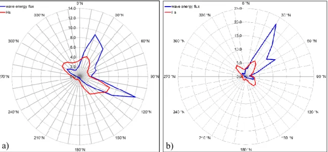
Figure 2-1. Satellite view of the unprotected coast near Senigallia. The up-right box shows the location of Senigallia Beach. The black box highlights the study area. 11 Figure 2-2. Location of the Senigallia beach (yellow circle), location of the Ancona RON buoy (red circles) and location of the points of the COAWST model (green circles). 14 Figure 2-3. Frequency distribution of significant wave height (red line) and wave energy flux (blue line): (a) RON buoy 1999-2006 & 2009-2013. (b) COAWST model 2015-2017,
P3. 15
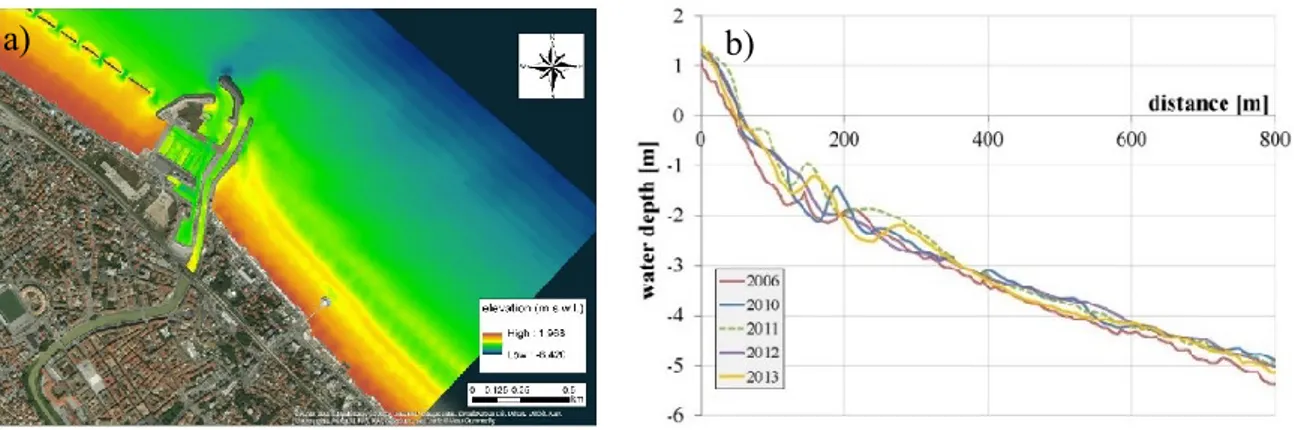
Figure 2-4. Time series of wave characteristics collected by the Meda Station from June 2018 to October 2018. The upper panel shows the significant wave height, the middle panel shows the wave peak period and the lower panel shows the wave peak direction. 16 Figure 2-5 - (a) Bathymetric survey of the study area, May 2013. (b) Changes of the
cross-shore profile highlighted from the available surveys. 19
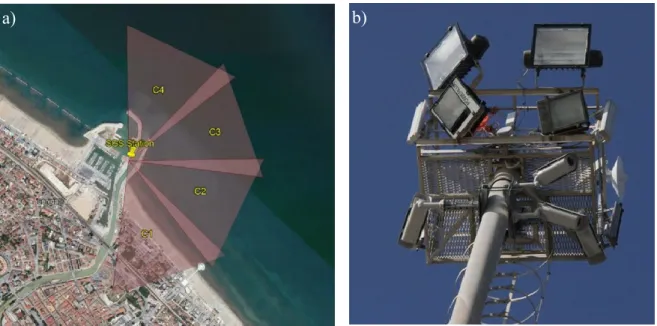
Figure 3-1 - a) General view of the Senigallia harbour showing the SGS Station position and the cameras field of view. b) The four cameras installed on the top of the tower. 22
Figure 3-2 – Particulars of the camera installation. 23
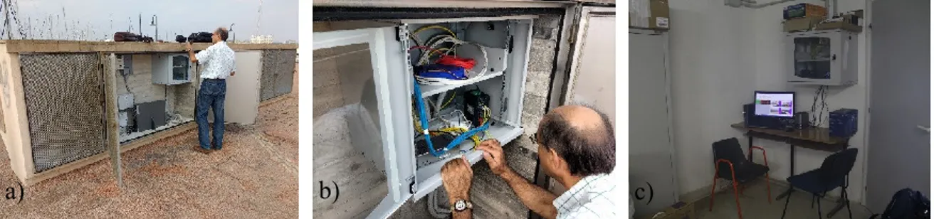
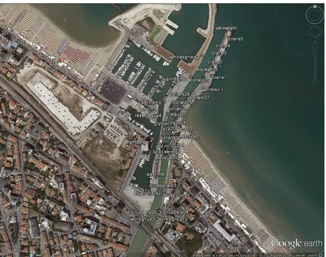
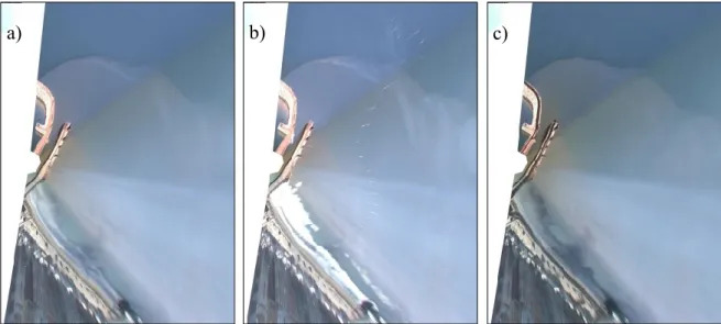
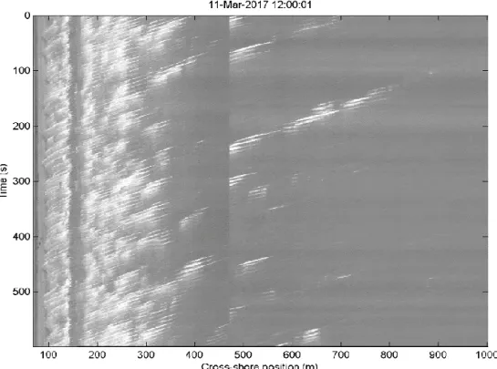
Figure 3-3 – a) Communication box. b) Camera trigger. c) Computer station. 23 Figure 3-4. Plan view location of the GCPs surveyed by means of the GPS technology. 26 Figure 3-5 – Merged and orthorectified images: a) Timex, b) Bright, c) Dark. 28 Figure 3-6 Example of stabilization effects. a) Target image (red) superposed to moving image (cyan). b) Target image (red) superposed to stabilized moving image (cyan). 29 Figure 3-7 – Example of a Timestack where the wave propagation and the swash motion
(50m<x<100m) are well visible. 30
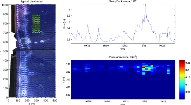
Figure 4-1 The left panel shows an example pixel array used for cBathy analyses: sampling pixels (blue dots, half shown), an example of analysis point (red asterisk) and pixels in the nearby region (green dots). The right panels show an example of offshore wave height (top) and of Process error, Q (bottom), found from bathymetric variability during the Sandy Duck field experiment, 1997. Adapted from Holman et al. (2013). 35 Figure 4-2 Measure of the tide elevation from the SGS Timex images. 37 Figure 4-3 – a) cBathy Phase II estimated bathymetry. The blue lines are the sections of survey profiles (2013), the red lines are the sections of the cBathy grid, and the black lines are the camera boundaries. b) Error Map (95% confidence intervals) from cBathy Phase II. Depth colormaps have blue for shallow and red for deep. The harbour is located in the
xiv upper part of the domain (y~-700m), while the Rotonda is located in the lower part
(y=0m). 39
Figure 4-4 – Comparison of estimated and measured bathymetry. The blue lines are the survey bed (2013) and the red lines are the cBathy estimated bed. The profiles are related
to the transects shown in Figure 4-3. 40
Figure 4-5 - Time series and profile at y=316m. The upper panel gives the Timestack, where the red dotted lines are the x-positions of the debug points. In the lower panel the blue line is the survey seabed (2013), the red line is the cBathy estimated bed and the grey
lines are the x-positions of the debug points. 41
Figure 4-6 - Phase maps for the range of frequencies selected in the setting file. 43 Figure 4-7 - a) Zoom of the ortho-rectified snapshot. The red dots are the points of the sampling grid (spaced 3m), the blue dots are the points of the sections, the green dots are the debug points and the black circles identify the wave crests. b) Zoom of the phase map
for the frequency 0.18Hz. 44
Figure 4-8 Comparison between observed and predicted phase and magnitude maps for the tile relative to the analysis point D (x=275m, y=-316m). The maps are ordered from the most coherent frequency (fB1) to the less coherent frequency (fB4). maxNpix=80 points.
47 Figure 4-9 Comparison between observed and predicted phase and magnitude maps for the tile related to the analysis point (x=275m, y=-316m). The maps are ordered from the most coherent frequency (fB1) to the less coherent frequency (fB4). maxNpix=500 points. 48 Figure 4-10 Profile at y=316m. The blue line is the survey bed (2013), the red line is the cBathy estimated bed with maxNPix=80, the green line is the cBathy estimated bed with maxNPix=500, the cyan line is the estimated bed using cBathy v1.2 and the grey lines are
the x-positions of the points used for the debugging. 49
Figure 4-11 Plots of: first dominant frequency of each point (top left panel), relative
wavenumber (top right panel) and gamma (bottom panel). 51
Figure 4-12 - In red the calculated values of wavelength for a period of 5.5s and the corresponding depth. The dotted black lines show the approximated position of these depths along the survey profile. The blue letters show the approximated position of some points of the debug analysis. The blue line is the survey profile (2013) while the brown line is the cBathy estimated profile. The green lines are the contours of the camera
resolution. 52
Figure 4-13 Resolution along the cross-axis of the cameras (normal to main axis of the camera). The black asterisk is the camera location. The black line is the 3 m contour. The
y-axis is inverted. 53
Figure 4-14 Resolution along the main axis of the cameras. The black asterisk is the camera location. The black line is the 3 m contour. The y-axis is inverted. 53 Figure 4-15 Resolution in cross-shore direction. The black asterisk is the camera location.
The black line is the 3 m contour. The y-axis is inverted. 54
Figure 4-16 Resolution in alongshore direction. The black asterisk is the camera location.
Figure 4-17 - Scheme of the way of the cameras look at the waves in relation to their
location. 57
Figure 4-18 – a) Example of peak shifting for case E01 with peak directions of 0° (red), 45° (blue), and 90° (green). b) Example of frequency directional spectrum (A20) designed
using equations (4.11) to (4.15). 60
Figure 4-19 - Optical images (upper panels) and estimated bathymetry (lower panels), for case E01, for wave angles equal to 0° (a,d), 45° (b,e), and 90° (c,f). The angles are positive in the counter-clockwise direction from the x-axis. The red arrows indicate the wave direction. The seed angle has been set coherent to wave propagation. 65 Figure 4-20 – Results of bathymetric error as function of difference between wave angle and camera viewing direction. a) analytical spectra A10, A20,A21, A22; b) analytical cases A10, A11, A12 and A13 with different directional spreading; c) observed spectra E01, E02, E03, E07 and E08; d) same as c) but includes case E05. 67 Figure 4-21 – Seed angle sensitivity for analytical (a-c) and experimental (d-f) cases with
wave angles of 0° (a,c), 45° (b,e), and 90° (c,f). 69
Figure 4-22 – For case E01, the residual calculated using (4.29) for wavenumbers (a,d), frequencies (b,e) and depths (c,f) are plotted. Only the first coherent frequency and one realization for waves coming from 0° (a-c) and 92° (d-f) is illustrated. Mean (*) and standard deviation (bars) of relative error (4.30) are shown for wavenumber (g) and
frequency (h) as a function of wave viewing direction. 71
Figure 4-23 – For case E01, the residual calculated using (4.29) for the seed analysis of wavenumbers (a,d), frequencies (b,e) and depths (c,f) are plotted. Only the first coherent frequency for seed equal to 0° (a-c) and 90° (d-f) is illustrated. Relative wavenumber (g) error is affected by seed angle, while frequency (h) is determined before the non-linear fit in step 1 of the cBathy algorithm and is therefore not sensitive to seed angle 72 Figure 5-1 – Extrapolation of intensity from imagery. Three Blimelines are identified in the images (green, violet and orange lines). The vertical continuous black lines indicate the location of three cross-shore sections (-500m, -400m, -300m) for which the sampling
intensity profile is shown (blue lines). 74
Figure 5-2. Example of bar crest identification from stabilized ortho-rectified Timex images and comparison with the bathymetric survey of 2013. Blue lines give the breaking lines from BLIM; red, yellow and green dots are, respectively, the location of the outer, intermediate and inner bar crests from the bathymetric survey. 76 Figure 5-3 Sandbars configurations occurring during the SGS station functioning. 79 Figure 5-4 Wave climate from the COAWST model. The three upper panels show the frequency distribution of significant wave height (red line) and wave energy flux (blue line), in the years 2015, 2016 and 2017 (respectively from left to right). The lower panel shows the time series of the significant wave height for the first six months of 2016. The variation of the colour indicates the wave direction. The numbers indicate the progressive
storms 81
Figure 5-5 - Sandbar position in relation to the wave climate. (a) Significative wave height from the COAWST model. The variation of the colour indicates the wave periods (light blue <5s, blue=5s, green=6, magenta=7s, red>7s). The numbers indicate the progressive storms. The vertical black lines indicate the days shown in the bottom panels. (b)-(f)
xvi breaker lines extracted from Timex images: blue, green and red lines are for inner,
intermediate and outer bars respectively. 82
Figure 5-6 Correlation between the mean sand bar location (upper panel) and the wave climate (lower panel), for the full analysed period. The numbers indicate the progressive storms. The yellow bands indicate the period in which the station did not work. 83 Figure 5-7 – Correlation of the cross-shore mean intermediate bar position (central panel), the alongshore variability (right panel) and the wave climate for year 2016 (left panel). The
numbers indicate the progressive storms. 84
Figure 5-8 From the upper to the lower panel: significant wave height time series from P3 of the COAWST model, the numbers indicate the progressive storms; total energy flux for each storm; cross-shore component of the energy flux; alongshore component of the
energy flux; duration of the storms in hours. 87
Figure 5-9 – Test1 (ESE) – Upper panel: seabed profile. Middle panel: wave height. Lower panel: mean undertow current. The vertical solid line is the breaking point, the vertical
dash-dot line is the end of the transition zone. 91
Figure 5-10 – Test2 (NNE) – Upper panel: seabed profile. Middle panel: wave height. Lower panel: mean undertow current. The vertical solid line is the breaking point, the
vertical dash-dot line is the end of the transition zone. 92
Figure 5-11 –Bathymetry and geometry used in the Boussinesq simulation. Points G1 and
G2 are two probes. 93
Figure 5-12 – Acceleration skewness recorded from gauge 1 (upper panel) and from gauge 2 (lower panel). The red lines represent the ESE storm while the blue lines represent the
List of Tables
Table 3-1 Examples of post-processed images (13 March 2017 h 13.00) 24 Table 4-1 – Example of setting parameters used to apply the cBathy algorithm to the
Senigallia site. 38
Table 4-2. Numerical results for the debug point D (x=275m, y=-316m). The depths are
not tide corrected yet. maxNpix=80 points. 47
Table 4-3 Numerical results for the debug point D (x=275m, y=-316m). The depths are not
tide corrected. maxNpix=500 points. 48
Table 4-4 - Celerity analysis, point D. 50
Table 4-5 - Summary of analysed sea states and parameters, from analytical source. For each case the table displays the index, the peak period, the significant wave height, the spreading parameter, the camera height, the camera tilt angle (fixed in the patches) and the
water depth. 58
Table 4-6 - Summary of analysed sea states and parameters, from EsCoSed experiment source. For each case the table displays the index, the peak period, the significant wave height, the wave energy, the camera height, the camera tilt angle (fixed in the patches), the
water depth, and the time of measurement. 58
Table 4-7 - Summary of cBathy parameters. The x-axis is the cross-shore direction, and
the y-axis is the alongshore direction. 63
Table 5-1 Wave characteristics of two representative storms from the COAWST model. Hs
is the significant wave height, Tp is the peak wave period, θ is the wave direction with
respect to the cross-shore direction, positive clockwise, looking towards offshore. Test 1 is the ESE storm n.6 of Figure 5-8, while Test 2 is the NNE storm n. 8 of Figure 5-8 88 Table 5-2 Results of the first net offshore transport analysis. Analytical model of equations
(5.9)-(5.18). 92
Table 5-3 Results of the net offshore transport analysis. Analytical model of equations (5.9)-(5.18) with increased longshore velocities by reflection off the river pier (equation
List of Symbols
(𝐹𝑥, 𝐹𝑦) cross-shore and the alongshore component of the energy flux (𝑈, 𝑉) 2D image coordinates
(𝑋, 𝑌, 𝑍) 3D world coordinates
(𝑥, 𝑦) cross-shore and alongshore coordinate (𝑈0, 𝑉0) image centre coordinates
(𝑓𝑈, 𝑓𝑉) focal lengths
(𝑥0, 𝑦0) global coordinates of the origin of the local coordinate system [xp, yp] pixel sampling array (cBathy)
[𝑥𝑚, 𝑦𝑚] user-defined analysis point (cBathy) D50 median-diameter of sediment
ℎℎ𝑜𝑢𝑟 current hourly estimates (Kalman filter)
ℎ𝑏 water depth at the breaking point
ℎ𝑝𝑟𝑖𝑜𝑟 previous running averaged bathymetry (Kalman filter)
ℎ𝑢𝑝𝑑𝑎𝑡𝑒 updated average depth (Kalman filter)
Ub depth-averaged time-mean undertow velocity
Ur mean velocity due to the surface roller
Uw mean velocity due to the Stokes drift Ω∗ dimensionless fall velocity
𝐴𝑛 amplitude of the noise signal in the frequency domain 𝐴 amplitude of the wave signal in the frequency domain
xx
𝐵∗ bar parameter
𝐵0 wave shape parameter for the undertow
𝐶𝑓 friction coefficient due to the waves and currents
𝐷0 normalization factor
𝐹𝑖 energy fluxes of each hour
𝐻𝑏 breaking wave height
𝐻𝑡 wave height at the end of the transition zone
𝐾1 constant (Taylor approximation)
𝐾𝑣 von Karman’s constant
𝑁ℎ number of hours
𝑁𝑠 elements of the transformed series 𝑇𝑧 mean zero-upcrossing period
𝑈𝑏′ maximum value of the undertow current
𝑈𝑏∗ friction velocity
𝑉𝑏
longshore velocity at the breaker line by considering the presence of horizontal mixing
𝑉𝑏′ maximum value of the longshore current
𝑉𝑜
maximum longshore velocity at the breaker line with no horizontal mixing
𝑐𝑔 group speed
𝑓𝑐 friction coefficient due to current 𝑘𝑑𝑒𝑒𝑝 deep water wavenumber
𝑘𝑠 roughness height of the stationary bed
𝑛𝐸 estimated value
𝑛𝑇 true value
𝑟𝑖 radiance incident ray
𝑟𝑛 vector normal to the wave sea surface
𝑠𝑘 image skewness
𝑣1 dominant eigenvector of the cross-spectral matrix 𝑣1′ phase of the dominant eigenvector
𝑤𝑠 sediment settling velocity
𝑥𝑠 offshore distance where the beach slope becomes very small 𝛼𝑐 camera azimuth or camera view direction
𝛼𝑛 wave propagation direction
𝛼𝑛 wave direction
𝛾𝑛 wave slope
𝜃0 offshore wave direction with respect to the cross-shore direction 𝜃𝑃 spectral peak direction
𝜃𝑏 wave angle at the breaking line
𝜌𝑎 water density
𝜌𝑠 particles density
𝜏𝑏 bed shear stress
𝜑𝑛 phases of the harmonic variability of the noise
𝜔′ angle of refraction
f frequency
fB1 most coherent frequency
ℎ still-water depth
ℎ𝑐 camera height
ℐ identity matrix
xxii lam1 normalized eigenvalues
maxNpix maximum number of points per tile ℛ Fresnel reflection coefficient
t time TR tide range α wave direction γ Gamma coefficient Γ Gamma Function ϕ iphase shift
𝐴 dimensional shape parameter (equilibrium profile) 𝐶 vector of camera centre in world coordinates 𝐷(𝑓, 𝜃) directional distribution
𝐸 wave energy
𝐸(𝑓) one dimensional, frequency dependent wave spectrum
𝐹 energy flux
𝐺 intensity signal from the frequency domain 𝐺(𝑓) coefficient (spectrum)
𝐻 local wave height
𝐻𝑠 significant wave height
𝐼 intensity signal from the time domain
𝐾 intrinsic matrix
𝐾𝑟 refraction coefficient 𝐾𝑠 shoaling coefficient
𝐿 wave length
𝑁 number of comparison values
𝑄 process error
𝑅 camera rotation matrix
𝑅𝑇𝑅 relative tide range
𝑆(𝑓, 𝜃) analytic frequency-directional spectra 𝑆𝑚𝑎𝑥 spectrum wave energy
𝑇 wave period
𝑇𝑝 spectral peak period
𝑉 longshore current
𝑊 Fourier series of the surface elevation
𝑐 wave celerity
𝑔 gravitational acceleration
𝑘 radial wavenumber
𝑚 bottom slope
𝑛 constant (equilibrium profile) 𝑟𝑀 roto-translation matrix
𝑠 spreading parameter
𝒞 cross-spectral matrix ()
𝒦 is the Kalman gain
𝛺 radial wave frequency
𝛽 Coefficient for considering the horizontal mixing
𝛿 height-to-depth ratio of breaking waves in shallow water 𝜂 sea surface elevation time series
𝜃 wave direction
𝜈 kinematic viscosity of water 𝜎 coefficient (spectrum)
xxiv 𝜏 camera tilt from horizontal
𝜑 phases of the harmonic variability of waves
𝜔 angle of incidence of the sky radiance with respect to the sea surface normal
Chapter 1 Introduction
1.1 Objectives and thesis outline
This thesis concerns the first application of the data coming from a new video-monitoring station (SGS station) installed in July 2015 at the Senigallia Harbor, Italy. The overall goal of this work is to improve the knowledge of the hydro-morphodynamics of a micro-tidal, estuarine sandy beach environment (Senigallia beach) that is typical of the beach near an estuary along the Adriatic coast (Italy). Notwithstanding the capability of SGS station to explore the physical processes that evolve both in the beach on the south side of the Senigallia harbour and in the mouth of the Misa River, the present thesis mainly focuses on improving the knowledge of the morphological features of the sandy beach by adding to traditional survey techniques new prospective of study deriving from the video-monitoring data.
Two main aspects have been investigated:
I) the study of the capability of the SGS data to estimate the water depth using cBathy (a widely used algorithm for depth-inversion) (see Chapter 4)
II) the study of the dynamics of a multiple sandbars system by using the bar line information coming from post-processed images of the SGS station (see Chapter 5)
In detail the thesis is organised in six chapters.
Chapter 1 (Introduction) introduces the main aspects and gives an historical overview of the remote sensing techniques used to study the nearshore zone, with a focus on the use of this technology to perform bathymetry reconstruction and bar evolution analyses.
Chapter 2 (The study area) describes, on the basis of previous studies and traditional survey techniques, the main hydrodynamic features and the morphological characteristics of the
2 Chapter 3 (The SGS station) introduces the SGS station and describes the installation, the data acquisition and the data post-processing analyses. All the post-processing products that are being elaborated are illustrated, with particular attention to those that are used in the analyses of this thesis.
Chapter 4 (Bathymetric Analysis) describes the first application of the SGS data to indirectly estimate the nearshore bathymetry. More in detail, Section 4.1 describes the widely used cBathy algorithm, while Section 4.2 shows the results of the application of cBathy to the SGS optical data. The implementation produced results that vary in quality as a function of the location and wave conditions and highlights an underestimation of the water depth over much of the domain. A debugging analysis performed to find the source of the underestimation is illustrated in Section 4.3. The depth underestimation has been mainly related to the difference between the wave direction and camera pointing direction. The relevance of this aspect has been analysed in depth using synthetic tests in Section 4.4. Chapter 5 (Sandbar analysis) describes the application of the SGS data to analyse the submerged nearshore sandbars behaviour. The capability of the station to support analyses of the evolution of a multiple bar system is investigated. The methodology used to extract information on the bar crest positions from the images collected by the cameras is first described in Section 5.1. Then, the observed bar morphology (Section 5.2) and the cross-shore mobility of the bars (Section 5.3) are discussed.
Chapter 6 (Conclusion) provides some final considerations, general conclusion and suggests some possible future development.
1.2 Remote Sensing to study the nearshore zone
The nearshore zone is the area of the sea that extends from the breaking line to the shoreline. It can be further divided into two different areas: the surf zone, where the waves break and the swash zone, where the waves reach the beach and move the instantaneous shoreline back and forth.
The hydro-morphodynamics of this area, where the most dissipation of energy occurs, is complex with physical phenomena evolving over a wide range of temporal and spatial scales. By entering in the shallow waters, the incident waves begin to fill the presence of the
seabed and become skewed and asymmetric, due to nonlinear effects. Then, the waves break, undergoing a high energy dissipation before they reach the beach. From the morphological point of view, waves can force both a net onshore sediment transport, in wave-averaged models related to the acceleration skewness (Hoefel and Elgar, 2003; Silva et al., 2011) and a net offshore sediment transport, largely induced by the wave undertow due to braking waves (Roelvink and Stive, 1989; Abreu et al., 2012). The interaction between waves, currents, and sediment transport leads to complex variability in the nearshore bathymetry, which is required to understand and predict all nearshore physical processes.
Since the coast area is highly anthropized and strategic for human activities, the knowledge of the dynamics of the nearshore environment is of great importance from the social, economic, and environmental points of view. For example, bathymetric change prediction is crucial to investigate coastal erosion, flood risk exposure and evaluate hazards associated to safety and infrastructure design and stability. To understand the behaviour of the coastal environmental, accurate physical measurement are necessary.
Traditionally, nearshore physical characteristics have been sampled by means of in-situ instruments, this involving the use of ships, jet skis or amphibious vehicles such as the Lighter Amphibious Resupply Cargo (LARC) and the Coastal Research Amphibious Buggy (CRAB). Shipboard single and multibeam echo sounding or sonar-equipped jet-skis are widely used, as well as monitoring buoys and poles. They can provide highly accurate measurements and are essential to know the hydro-morphological features of the nearshore region. However, traditional methods are expensive, time-consuming, sometimes limited to calm sea conditions and inapplicable to the very shallow waters. This results in spatial and temporal resolution lower than necessary for the observational and modelling needs. Monitoring the beach behaviour under both seasonal and extreme events is important to facilitate coastal management decisions (Davidson et al., 2007) and also to implement beach nourishment projects (Hamm et al., 2002; Ojeda and Guillén, 2006).
Over the last decades, remote sensing techniques, such as LIDAR, Radar and optical sensors, have been developed as alternative tools to monitor the coastal evolution (Hamm et al., 2002). Remote sensing methods offer the capability to collect a high volume of data at high temporal and spatial resolution with relatively low cost and over a long period. For example, remote sensing techniques can indirectly estimate the water depth and fill spatial and
4 methods are not limited by high-energy storms and, therefore, may be employed when more traditional sampling methods must be abandoned.
In general, there are two types of remote sensing technologies: active sensors, such as Radar and Lidar, which emit a signal and evaluate the time delay between emission and return, and passive sensors, which gather the radiation emitted or reflected by an object, such as the sunlight reflected by the sea surface and measured through a camera.
Nowadays, use of imaging methods is very common and in particular optical data are widely employed all over the world. The use of images to study the nearshore zone dates back to the thirties, when aerial photography was first used to map the coastline. Then, coastal remote sensing was developed to quantify hydro-morphodynamic characteristics from shore-based video observations using photogrammetric and computer vision techniques. Since the eighties these new methods developed at the Coastal Imaging Lab (CIL) of the Oregon State University led to the network of the Argus coastal monitoring stations (e.g. Holman and Stanley, 2013) and to the Coastal Imaging Research Network (https://coastal-imaging-research-network.github.io). An Argus station is a land-based automated and unmanned station programmed to acquire and return optical remote sensing data in sites of research interest (Holman and Stanley, 2007). It is typically composed of a number of video cameras mounted on an elevated position and connected to a host computer that controls the acquisition and storage of data. The hourly data collection mainly consists of a snapshot image, which shows the general condition, a ten minutes time exposure image, which averages the light intensity signal on each pixel, and the variance image, which shows the variance of the intensity signal during the recorded time. These oblique images can be geo-referenced and rectified using standard photogrammetric techniques to obtain plan view images that allow to quantify the image features. Furthermore, time series of pixel intensity can be collected through specifically-designed sampling schemes.
The first Argus station was installed at Agate Beach on the Oregon Coast in 1992 and presently, shore-based video systems are widely used in coastal research in many locations all over the world. In Italy, the first Argus station was installed in the North Adriatic coast at Lido di Dante beach in 2003 (Archetti, 2009, Armaroli and Ciavola, 2011). Subsequently, other video-monitoring stations, based on EVS (Erdman Video System) were installed in many sites along the peninsula, among others, at Igea Marina (RN), Sabaudia (LT), Terracina (LT), Pineto (TE), Senigallia (AN). These installations have been used to study
the coastline evolution and monitor the effects of nourishment and coastal defence works (Parlagreco et al., 2011). A new video monitoring station, called the “Sena Gallica Speculator” (SGS), was installed in July 2015 at the Senigallia harbour, central Adriatic, as part of the Estuarine Cohesive Sediments (EsCoSed) project (Brocchini et al., 2015). SGS is not part of the Argus network but it was designed on the bases of typical Argus systems. SGS is equipped with four cameras located on the top of a 25m high tower. Unlike Argus stations, which store only single images products and isolated pixel time series, ten minutes of full frame images data are being collected at 2Hz every hour, during daylight hours, and then post-processed. Like other video monitoring stations, SGS aims to support coastal, estuarine, and riverine studies in site of scientific interest.
The concept at the basis of the use of video monitoring imagery to study nearshore processes is that a physical phenomenon can be investigated through images, if it can be discerned visually (Holman et al., 1993; Holland et al., 1997). Fortunately, many nearshore processes have a visual manifestation, therefore the video-monitoring technique provides indirect measurement of the nearshore characteristics. For example, incoming waves are visible on the optical imagery, thus their period, wavelength and direction can be evaluated (Holman and Stanley, 2007). In the same way, preferential breaking areas appear on the time exposure images as bright bands indicating position of submerged sandbar (Lippmann and Holman, 1990). In general, the challenge is to extract accurate quantitative information of hydrodynamic and morphological features from optical signatures visible on the images. In the last decades, many algorithms for the estimation of different nearshore measurements have been developed and currently optical remote sensing is a powerful tool for sampling the nearshore environment (Holman and Stanley, 2007).
1.2.1 Remote sensing for bathymetry reconstruction
Quantifying bathymetric changes is crucial to support navigation and engineering projects, as well as to understand erosion and accretion processes of the beach. Prediction skill of forecasting models increases with more accurate bathymetric boundary conditions (e.g. van Rijn et al., 2003; Holman et al., 2014; Holman et al., 2016). High-resolution coastal elevation data are also necessary to achieve an accurate assessment of coastal flood risk (Beck et al., 2018).
6 In the last decades, thanks to remote sensing techniques, significant advances have been made in achieving nearshore bathymetry information. Each remote sensing tool has its own accuracy and limitations, and many alternatives are available (Gao, 2009). For clear water columns, where the bottom is visible, Light Detection and Ranging (LIDAR) is an accurate and popular tool to sample the bathymetry (Irish and Lillycrop, 1999). But for turbid water columns, where the bottom is not visible, the LIDAR cannot be used and other methods must be adopted. Another powerful tool to indirectly estimate the bathymetry is the X-band marine radar because wave parameters can be mapped from radar images and used in inversion algorithms based on linear wave theory (Bell, 1999). While the X-band radar can cover areas of a few kilometres giving appropriate results in to the very shallow-water zone, optical videos are typically used to collect data in shallow water because, in view of the high temporal and spatial resolution, they allow to properly extract information also over complex morphologies.
Since in turbid waters the surface signatures dominate, many authors studied the morphology evolution analysing the breaking wave patterns, visible on optical time-averaged images as high-intensity bands (Lippmann and Holman, 1990; van Enckevort and Ruessink, 2001, Aarninkhof et al., 2005). Another particular technique related sub-areal topography to shadows falling across a beach (Holman et al., 1991), while Holland and Holman (1997) have shown how stereo imagery of the moving swash could yield information on foreshore topography. Intertidal bathymetry could be measurement also by mapping shoreline contours over one tidal cycle (Plant and Holman, 1997; Aarninkhof et al., 2003).
Alternatively, nearshore bathymetry can be estimated using depth-inversion algorithms, based on the inversion of the dispersion relationship, which exploits the wave celerity observed by optical imagery. Depth-inversion method is currently one of the most frequently used video-based remote sensing methods to estimate nearshore bathymetry in the presence of surface gravity waves. This approach is based on the linear (e.g. Stockdon and Holman, 2000), nonlinear (e.g. Catálan and Haller, 2008), or extended Boussinesq dispersion equations (e.g. Misra et al., 2003). Two different approaches can be used to estimate the wave celerity, namely the time domain inversion (Almar et al., 2009) and the frequency domain inversion (Stockdon and Holman, 2000). The temporal method computes a time-domain cross-correlation between neighboring positions to estimate the wave celerity
(Almar et al., 2009), while the spectral method uses a cross-spectral correlation to estimate the wave celerity (Plant et al., 2008). Both approaches result in depth estimates with similar accuracy given synthetic optical video data (Bergsma and Almar, 2018). Among the linear depth inversion algorithms that use the spectral method to estimate the wave celerity, the open source depth-inversion algorithm known as cBathy (Holman et al., 2013) (https://github.com/Coastal-Imaging-Research-Network/cBathy-toolbox) has become one of the most widely used depth inversion algorithms (e.g. Holman and Stanley, 2013; Radermacher et al., 2014; Sembiring et al., 2014; Méndez et al., 2015; Bergsma et al., 2016; Holman et al., 2017; Rutten et al., 2017; Bergsma and Almar, 2018; Brodie et al., 2018; Zuckerman et al., 2018).
1.2.2 Remote sensing for bar evolution
A very important feature of natural beaches is the presence of particular seabed perturbations called sandbars. A submerged sandbar is a persistent accumulation of sand on the seabed below sea level (Holman and Sallenger, 1993). The nearshore zone of sandy unprotected beaches is often characterized by the presence of these morphological patterns. Some empirical parameters, such as the dimensionless fall velocity Ω (Wright and Short, 1984) and the bar parameter 𝐵∗ (Short and Aagaard, 1993), can be used to classify beaches where
single (2<Ω < 6) and multiple (𝐵∗ > 50) sandbars can evolve.
Accurate knowledge of submerged bar behavior is crucial first because sandbars are natural barriers to protect the coast from strong storm actions, which may cause significant beach erosion. Since submerged sandbars evolve in shallow waters, the incoming waves break preferentially near the ridge of the bars, inducing an important dissipation of the wave energy before the waves impact the shore. Such wave energy dissipation is also an important natural protection mechanism that improves the beach resilience. Moreover, for a proper management of sediment budgets, the presence of sandbars must be taken into account, since they involve significant volumes of mobile sand and have an important role on the sediment transport.
Nearshore submerged sandbars can exhibit very complex morphological states. They can occur as a single feature or as a multiple bar system and they can be alongshore uniform (2D bars) or present an intricate alongshore variability (variety of 3D bars). The mutual
8 interaction between sand transport, waves and currents generate a perpetual variability of sandbar systems, which are characterized by both cross-shore and alongshore motions. These changes may be affected by single storm events or dominated by seasonal cyclicity. Therefore, the study of sandbar behavior must be carried out analyzing phenomena with time scale varying from hours to months or years. In this respect it is difficult to understand the sandbar dynamics only on the basis of in situ traditional measurement. For these reasons the remote sensing technique may help gather useful information to study sandbar evolution and the related beach morphology. A video monitoring station, in fact, can observe a bar system for a very long period and, at the same time, with an hourly sampling resolution. Given the scientific and social importance of understanding the behaviour of sandbars and given the potentiality of video monitoring systems, many studies were developed in the past decades to properly identify sandbar features from optical images.
Remote monitoring of sandbar morphology is based on the observation that more waves break over the shallows of the bar than over the surrounding areas (Lippmann and Holman, 1990). Time exposure images, which are a classical product of video-monitoring stations, are a useful tool to highlight wave breaking patterns, because the areas of preferential breaking are displayed on these images as white bands. Lippmann and Holman (1990), first developed a technique that allows to estimate the sandbar position on the basis of the patterns of incident breaking waves. Their assumption is that light intensity recorded on the camera varies with the dissipation of the incident wave energy and they regarded the energy dissipation as a proxy to measure of bottom topography (Lippmann and Holman, 1990). Many approaches to sample bar crest location from images have been developed since then. A widely used algorithm, implemented also in the Argus toolbox Barline Intensity Mapper (BLIM), is the algorithm developed by Van Enckevort and Ruessink (2001).
This technique provides quantitative information on both cross-shore and longshore bar crest location and is commonly used to monitor submerged bar systems and nourishments in countless sites all over the world. The accuracy of video-based estimation of the bar location depends on the relationship between the maximum video image intensity and the seabed morphology and should be evaluated for each particular site. Focusing on the Mediterranean area, Ribas et al. (2010) confirmed the suitability of the video-monitoring technique to study bars and terraces on the micro-tidal beach of Barcelona. In the present thesis the barred
beach of Senigallia (Italy) is studied using the optical data coming from the new video-monitoring station, SGS.
Chapter 2 The Study Area
2.1 The Senigallia Beach
The Italian coast of the central Adriatic Sea is predominantly characterized by sandy and low-sloped beaches periodically separated along the coast by the mouths of rivers that flow from the mountains to the sea, in west-to-east direction. The coastline is highly anthropized and the beach is commonly used for commercial and touristic activities. To preserve the littoral area from both inundation and erosion risks, a number of hard defence structures were placed along the coast over the years. This thesis focuses on a stretch of coastline representative of those Adriatic beaches that are near to river mouths.
The study area is located in Senigallia (AN, Italy) about 30 km north of the Conero promontory. The coast is characterized by a very mildly sloping sandy beach and extends on southern side of the Senigallia Harbour, from the jetty to the Rotonda pier (Figure 2-1).
Figure 2-1. Satellite view of the unprotected coast near Senigallia. The up-right box shows the location of Senigallia Beach. The black box highlights the study area.
This area is the northern portion of a 12 km long stretch of natural coast, one of the few stretches of the Region coastline not protected by hard defence structures. Hence, the area represents a good site to study coastal processes typical of the Central Adriatic coast.
12 Moreover, the port of Senigallia is a typical Canal Harbour due to the presence of the mouth of the Misa River, and this allows to study also riverine and estuarine processes.
The coastline of the analysed area extends in the north-south direction with a rotation of about 47° from the north (Figure 2-2). The observed beach is characterized by medium (𝐷50
= 0.25-0.5mm) to fine (𝐷50 = 0.125-0.25mm) sand in its emerged profile and by fine sand in its subaqueous part. The sediment size of the submerged beach decreases moving southward. The swash zone is characterized by slopes ranging from 1:30 to 1:40 with an array of submerged bars in water depths 0 to 3 m. Depths deeper than 3 m are characterized by slopes of 1:200 (Postacchini et al., 2017).
The beach of Senigallia is a wave-dominated and micro-tidal environment (tide range<2m) with sea level ranging between -0.6 m and +0.6 m and a maximum tidal excursion that does not exceed 60 cm. Information of tide levels is obtained from a tide gauge located inside the Ancona Harbour and part of the Italian National Tide Gauge Network (RMN).
The study area is constrained by two rigid structures: the Senigallia Harbour in the northern part and the Rotonda pier in the southern part. The presence of the Rotonda pier does not significantly affect the evolution of the beach while the larger jetty of the Harbour induces a curvature of the shoreline in the northern part of the domain. The presence of the Harbour complicates also the hydrodynamics of the area because the waves coming from the ESE direction impact onto the walls and there get reflected.
The sediment transport of this area is influenced by both the wave motion and the Western Adriatic Coastal Current (WACC) that drives the sediment southward (Harris et al., 2008; Sherwood et al., 2004). Moreover, the freshwater discharge of the Misa River estuary transports sediments down to the river mouth and to the nearshore region, especially during the wintertime (Brocchini et al., 2015; Brocchini et al., 2017).
2.1.1 Wave climate
Knowledge about the wave climate of the analysed area derives from historical time series collected by the Ancona buoy of the Italian Data Buoy Network (RON). The Ancona buoy (red circles in Figure 2-2) was installed in March 1999, at around 30 km far from the shore, its location been slightly modified during 2000. The available data consists of two time series: from 1999 to 2006 and from 2009 to 2013. The buoy is currently out of service.
Previous studies (Postacchini et al., 2017) evaluated the overall wave climate on the bases of the significant wave height, peak period and direction provided by the Ancona Buoy every half hour. They highlighted that the wave climate in Senigallia is characterized by storm waves coming from two main directions: ESE (forced by Scirocco winds) and NNE (forced by Bora winds). The Bora is a cold wind very frequent and intense during winter. Given the narrow and elongated shape of the Adriatic Sea this wind has a relatively short fetch and generates short, steep and high waves that propagate almost perpendicular to the coast. The Scirocco is a warm wind coming from south-east and approaching the coast with wide angles. It has a longer fetch that allows long and less steep waves. It is common during summer and it is characterized by a surge larger than that typical of the Bora storms. Moreover, the storms coming from ESE are more suited to produce infragravity waves (Brocchini et al., 2017). These two types of storms are not a seasonal characteristic (summer condition -winter conditions). On the opposite, storms with different directions, due to an alternation of Bora and Scirocco winds, can occur during the same season. In general, wintertime is characterized by severe storm events while the summertime generally has milder wave conditions.
Since the Ancona Buoy stopped working in 2013 the data coming from the new video monitoring station (installed in 2015) must to be correlated with other available data sets of wave characteristics.
The closest location where wave time series are collected is at Cesenatico (Cesenatico Buoy in the Emilia Romagna Region). It is located 80 km north of Senigallia, at a distance of 8 km from the beach and placed in 10 meters deep waters. Unfortunately, results of wave frequencies and the inspection of the simultaneous wave time series collected in Ancona and Cesenatico reveal significant differences in the wave climate. Specifically, the waves at Cesenatico come mainly from the northeast sector, while the Ancona climate is characterized by the mentioned two main wave directions. Furthermore, the Cesenatico Buoy is located in shallower waters than the Ancona Buoy; therefore, the waves incoming from different sectors are rotated by refraction and focused in the cross-shore direction.
14
Figure 2-2. Location of the Senigallia beach (yellow circle), location of the Ancona RON buoy (red circles) and location of the points of the COAWST model (green circles).
Another opportunity is to use data extracted from the COAWST Model, a global circulation model available for the Adriatic Sea. COAWST is a Coupled Ocean–Atmosphere–Wave– Sediment Transport modelling system based on the Regional Ocean Modelling System (ROMS) and Simulating Waves Nearshore (SWAN) system. The model covers the northern Adriatic Sea and it has a grid resolution of 1 km. Three points of the model grid are analyzed in the present thesis: P3, P2 and P1 placed on waters of 50 m, 10 m and 5 m depth, respectively (Figure 2-2). Time series of the root-mean-square wave height, peak wave period and angle of wave incident with respect to north are available from 2015 to 2017. A comparison of the wave frequency distribution with reference to the direction of propagation available from the Ancona Buoy and COAWST (plotted with red lines in Figure 2-3), reveals that the model correctly reproduces the typical distribution of waves for this site. However, the distribution of the wave energy flux (represented with blue lines in Figure 2-3) predicted by the model is mainly concentrated from NNE and ENE, while no storms were generated by the Scirocco wind, which are typically the most energetic storms for that area. This may be related to the reduced length of the modelled time series. In fact, the wave
climate of this area has not a seasonal behaviour and some differences in frequency distribution of the wave energy flux can occur from year to year. Analysing in more detail the single years, we find that only in 2016 a 5% portion of the wave energy came from the ESE direction. In view of the above, the data extracted from the COAWST model have been mainly used for the analyses that follow.
Figure 2-3. Frequency distribution of significant wave height (red line) and wave energy flux (blue line): (a) RON buoy 1999-2006 & 2009-2013. (b) COAWST model 2015-2017, P3.
From June 2018 a new data set of wave characteristics has become available from the Meda Station. The Meda Station is part of the weather monitoring network of the ISMAR, the Italian Institute of marine science. It was installed in July 1988 and it is located at around 1.2 nautical miles from the Senigallia coast, at around 12 m water depth (43 45.350N - 013 12.540E WGS84). The station traditionally collects weather and oceanographic data such us the velocity and the direction of the wind, atmospheric pressure, temperature and salinity of the sea water. At the end of May 2018, thanks to a collaboration between ISMAR and the Department of Civil and Building Engineering and Architecture of the Università Politecnica delle Marche, funded within the ONRG-MORSE project, a new ADCP was installed to measure wave characteristics. Therefore, beyond other collected data, the significant wave height, wave peak period and wave peak direction are now available. Figure 2-4 shows the time series of the main characteristics of the waves currently collected by the Meda Station. These measurements are available from June 2018 to October 2018.
16
Figure 2-4. Time series of wave characteristics collected by the Meda Station from June 2018 to October 2018. The upper panel shows the significant wave height, the middle panel shows the wave peak period and
the lower panel shows the wave peak direction.
2.1.2 Bathymetric features
A general description of the morphology of the beach can be carried out by means of synthetic parameters, such us the dimensionless fall velocity Ω∗ (Wright and Short, 1984),
the bar parameter 𝐵∗ (Short and Aagaard, 1993) and the relative tide range 𝑅𝑇𝑅 (Masselink
and Short, 1993), which allow to classify the state of the beach:
Ω∗ = 𝐻𝑏 𝑤𝑠𝑇 , (2.1) 𝐵∗= xs g 𝑚 𝑇2 , (2.2) 𝑅𝑇𝑅 =𝑇𝑅 𝐻𝑏 , (2.3)
where 𝐻𝑏 is the breaking wave height, 𝑇 is the wave period, 𝑥𝑠 is an offshore distance corresponding to a specific depth at which the beach slope becomes very small, 𝑔 is the gravitational acceleration, 𝑚 is the bottom slope and 𝑇𝑅 is the tide range. The settling sediment velocity, 𝑤𝑠, was evaluated with the Zanke (1977) formulation, valid for sediment diameters in the range 0.1 𝑚𝑚 − 1 𝑚𝑚:
𝑤𝑠 = 10 𝜈 𝐷50(√1 + 0.01𝑔𝐷503 (𝜌 𝑠− 𝜌𝑎) 𝜈2𝜌 𝑎 − 1) (2.4)
where 𝜈 is the kinematic viscosity of water, 𝐷50 is the sediment median-diameter, 𝜌𝑠 is the particle density, 𝜌𝑎 is the water density. Using 𝜈 = 10−6 𝑚2/𝑠, 𝐷50 = 0.2𝑚𝑚, 𝜌𝑠 =
2650 𝑘𝑔/𝑚3 and 𝜌
𝑎 = 1000 𝑘𝑔/𝑚3, the settling velocity is 𝑤𝑠 = 0.0257 𝑚/𝑠.
For a general classification, frequent values of the above-mentioned quantities are used. In particular, for a typical storm condition it is 𝐻𝑏= 3 𝑚, 𝑇 = 7.5 𝑠, 𝑥𝑠 = 600 𝑚, 𝑚 = 0.0062. Therefore, the mentioned synthetic parameters are: Ω = 15.5, 𝐵∗ = 175 and
𝑅𝑇𝑅 = 0.2. Using mean wave condition( 𝐻𝑏 = 1𝑚 and 𝑇 = 7 𝑠), the mentioned synthetic parameters are: Ω∗ = 5.5, 𝐵∗ = 200 and 𝑅𝑇𝑅 = 0.6.
The dimensionless fall velocity, 𝛺∗, takes into account both wave characteristics and
sediment characteristics (Wright and Short, 1984). Values that exceed 6 are traditionally correlated with dissipative conditions and a stable morphodynamic state. In this kind of environment submerged bars may be present and rips are usually absent (Masselink and Short, 1993). Following the conceptual beach model of Masselink and Short (1993), who analysed also the role of the tide, the above calculated values of dimensionless fall velocity, 𝛺∗ , and relative tide range, 𝑅𝑇𝑅, allow to classify the beach of Senigallia as a barred
dissipative beach. The possible number of sandbars may be predicted using the dimensionless bar parameter, 𝐵∗, which takes into account both the nearshore geometry and
wave period (Short and Aagaard, 1993). The value of 𝐵∗ estimated for the Senigallia beach,
indicates the likely presence of three bars.
The results of this simple empirical analysis are confirmed by the morphological features observed by in-situ surveys. The beach of Senigallia was frequently sampled with traditional bathymetric surveys over the last two decades, also thanks to the monitoring program established to control the effects of the port expansion works.
In June 2006, the Marche region promoted a topographic and bathymetric monitoring plan for an area spanning 4.3km in the longshore and reaching a depth of 6m. The topographic survey was performed over the emerged part of the beach, the swash zone and for the first meter depth of the submerged beach. The sampling of the shoreline was made during calm sea conditions and the survey was executed along sections perpendicular to the coast, spaced of about 50m. At the same time, a bathymetric survey was performed for the submerged part of the analysed area by means of a Multibeam system with high accuracy (5cm RMS). The data acquisition system produced a three-dimensional digital terrain model (DTM).
18 Between 2010 and 2013, after the modification of the harbour entrance, four annual bathymetric surveys were performed: in February 2010, in February 2011, in April 2012 and in May 2013. These surveys were promoted by the Municipality of Senigallia and were carried out for a longshore length of 2.5km, up to the bathymetric of -6m. Also in these cases, digital terrain models ware obtained. Then, using ESRI ArcGIS 9.3, 18 cross-sectional profiles were extracted. The first 8 transects have been used in the present thesis as bathymetric benchmarks for the performed analyses.
The bathymetries surveyed in 2006, 2010, 2011, 2012 and 2013 have shown a general invariance of the seabed profile and the presence of a system of three submerged sandbars in a water depth of around 0-3m (Soldini et al., 2014; Postacchini et al., 2017). The short-to medium-term variability observed in the surveys is related to the evolution of submerged bars but the previous analyses did not resolve the storm-time variability of the bar system, which needs to be further investigated. Instead, the long-term stability of the seabed has been confirmed by a good adaptation of the beach to the Dean-type equilibrium profile (Soldini et al., 2014). The equilibrium beach profile (Dean, 1991) describes the balance of a shore-normal transect of a natural beach between erosive and accretive forcing:
ℎ = 𝐴 𝑥𝑛 (2.5)
where ℎ is the still-water depth and 𝑥 the cross-shore coordinate. The constant 𝑛 is equal to 2/3 (Dean, 1991), while the dimensional shape parameter 𝐴 can be directly related to the median grain diameter (Hanson and Kraus, 1989). The 𝐴 parameter can also be calculated from experimental data, by means of techniques of best fitting.
Figure 2-5 shows an example of the DTM obtained from an in-situ bathymetric survey (May 2013) and the variability of the beach cross-shore profiles, which also display the long-term stability of the beach and the short-term variability of the bar system.
Figure 2-5 - (a) Bathymetric survey of the study area, May 2013. (b) Changes of the cross-shore profile highlighted from the available surveys.
Chapter 3 The SGS Station
3.1 Features and installation
A new shore-based video monitoring station was designed to monitor the nearshore area of a typical beach along the Middle Adriatic Sea. It was installed at the Senigallia town with the aim to observe both an unprotected stretch of a low-sloped sandy coast and the downstream part of an estuary. The station is named Sena Gallica Speculator (SGS) from the Latin name of this site.
The SGS station was installed in July 2015 as part of the Estuarine Cohesive Sediments (EsCoSed) project (Brocchini et al., 2015). The installation has been made possible thanks to the collaboration between the Department of Civil and Building Engineering and Architecture of the Università Politecnica delle Marche and the U.S. Naval Research Laboratory. The objective of the EsCoSed project was to better understand coastal, estuarine, and riverine processes at the Misa River mouth. For this purpose, also two field experiments were performed to investigate summertime (September 2013) and wintertime (January 2014) conditions (Brocchini et al., 2015; Brocchini et al., 2017).
The SGS station is part of the Coastal Imaging Research Network (CIRN), which grew out of the Argus camera system from Coastal Imaging Lab at Oregon State University. It has drawn inspiration from the classical Argus station structure but it is not part of the Argus Network. The main differences with traditional Argus stations regard the type of data storage and the logistics of the archive. In contrast to traditional Argus imaging stations, which collect only subsampled pixel time series, full frame video data are collected from this facility. The raw video data are then elaborated in post-processing. This allows gathering more general information that can be differently processed on the basis of the specific study at hand, but, obviously, this generates also the logistics issue of storing such large data
22 The SGS station is designed to be a long-term facility. It is located at the North pier of the port channel of Senigallia (Figure 3-1). The importance of the location is related to the possibility to observe both the nearshore and the estuary of the Misa River. The station is mainly composed by four cameras located on the top of a tower, at 25m above mean sea level (Figure 3-1). Three cameras face South toward the 500 m long unprotected beach between the harbour jetty and the Rotonda pier, this allowing to study the hydro-morphodynamics of the nearshore zone. The fourth camera faces northward toward the estuary of the Misa River; therefore the data recorded by the cameras represent a major source of information to improve also knowledge on estuarine dynamics.
Figure 3-1 - a) General view of the Senigallia harbour showing the SGS Station position and the cameras field of view. b) The four cameras installed on the top of the tower.
The four cameras installed on the top of the tower are FLIR/Point Grey Grassopher3 with 9 MP resolution (3376 × 2704). The lenses are CF12.5HA-1 with 12.5 mm focal length and 49 mm linear polarizing filter. The cameras are placed inside CRONO CPK405PoE housings (Figure 3-2). The camera field-of-view is 53° for an overall angle of 200°. The resolution is between 0.05 m and 0.50 m and the useable distance is 700 m. Particular attention was made to obtain a suitable overlap of the field of view of each single camera. In November 2016, the cameras have been rotated to better superpose the fields of view and not lose information.
Figure 3-2 – Particulars of the camera installation.
Through a pair of cables, the camera system is connected to a communication box located 60 m far from the tower, where an external trigger (custom built by Naval Research Lab, US) synchronizes the camera acquisition (Figure 3-3). Then the system is linked to a computer where a software (Streams 7) controls the data collection and archive (Figure 3-3).
Figure 3-3 – a) Communication box. b) Camera trigger. c) Computer station.
For each recording hour, the data collected from each camera consists in a video and a snapshot. The acquisition occurs during daylight hours, from 5:00 AM to 5:00 PM UTC, for a total of thirteen videos and thirteen snapshots a day, for each camera. A video consists of the first ten minutes of an hour and it is collected at 2Hz. The Snapshot image is the first frame of a video and it is saved to get a rapid overall visual assessment of the dataset. Videos and snapshots are temporarily stored on a 8TB external drive and periodically uploaded on a repository server located at the Università Politecnica delle Marche. The data recorded from the cameras are archived based on typical storage and file naming Argus convention. A large amount of data is already available and it grows every day as the station is currently working. From 2015 to 2017 the gaps of the data collected from the SGS station were around 20% of the total number of days.
a) b) c)
24
3.2 Data post processing
The hourly videos and snapshots recorded from the SGS station are post-processed using the Argus Database, the CIL toolbox and some custom Matlab© Codes. The post-processing of the SGS raw data includes the production of classical Argus images.
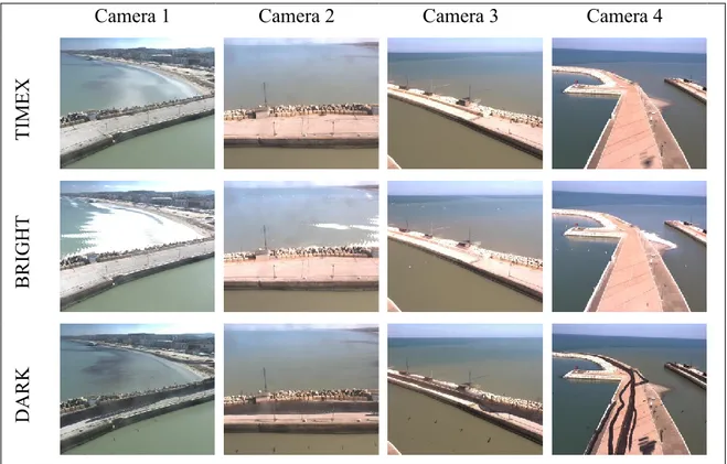
First, the videos of each hour and each camera, are elaborated to obtain a 10-minute time-exposure image, a darkest image, a brightest image and a full time series from the recorded period for a selected grid of pixels. In a second step, the processed images, together with the snapshots, are merged and ortho-rectified to obtain other five products per hour: a panoramic image and four (snapshot, time-exposure, darkest and brightest) plan view images. All these productions generated a continuously updated database (Table 3-1, Figure 3-5, Figure 3-7). These post-processing analyses are currently performed from July 2015, when the camera started to work, to November 2017.
More in detail, the time exposure (or Timex) images are created by averaging the intensity values of each pixel over the 10-minute sampling period (Table 3-1).
Table 3-1 Examples of post-processed images (13 March 2017 h 13.00)
Camera 1 Camera 2 Camera 3 Camera 4
TI MEX B R IG HT DA R K