ISSN-1697-1523 eISSN-1139-3394 DOI:10.3369/tethys.2010.7.02 Journal edited by
ACAM
A performance evaluation of MM5/MNEQA/CMAQ air quality
modelling system to forecast ozone concentrations in
Catalonia
R. Arasa1, M. R. Soler1, S. Ortega2, M. Olid1and M. Merino1
1Department of Astronomy and Meteorology, Universitat de Barcelona, Avinguda Diagonal 647, 08028 Barcelona 2Department of Physics and Nuclear Engineering, Universitat Polit`ecnica de Catalunya, C/ Urgell 187, 08036 Barcelona
Received: 27-V-2009 – Accepted: 2-XII-2009 – Original version
Correspondence to:[email protected]
Abstract
We examine the ability of a modelling system to forecast the formation and transport of ozone over Catalonia, at the NE of the Iberian Peninsula. To this end, the Community Multiscale Air Quality (CMAQ) modelling system developed by the United States Environmental Protection Agency (US EPA) and the PSU/NCAR mesoscale modelling system MM5 are coupled to a new emission model, the Numerical Emission Model for Air Quality (MNEQA). The outputs of the modelling system for the period from May to October 2008 are compared with ozone measure-ments at selected air-monitoring stations belonging to the Catalan Government. Results indicate a good behaviour of the model in reproducing diurnal ozone concentrations, as statistical values fall within the EPA and EU regulatory frameworks.
Key words: air quality modelling, meteorological modelling, CMAQ, ozone, evaluation
1 Introduction
As a result of combined emissions of nitrogen oxides and organic compounds, large amounts of ozone are found in the planetary boundary layer. Tropospheric ozone is considered one of the worst pollutants in the lower tro-posphere. At high concentrations ozone is toxic to plants and reduces crop yield (Guderian et al., 1985; Hewit et al., 1990; Zunckel et al., 2006). Sitch et al. (2007) suggest that the effects on plants of indirect radiative forcing by ozone could contribute more to global warming than the direct radiative forcing due to tropospheric ozone increases. Ozone is a respiratory irritant to humans, and it damages both natural and man-made materials such as stone, brick-work and rubber (Serrano et al., 1993). All these harmful effects are significant in Southern Europe (Silibello et al., 1998; Grossi et al., 2000; San Jos´e et al., 2005) as in summer solar radiation exacerbates the effects of ozone. This is the case in areas of northern Spain located near urban and industrial areas, and especially those lying downwind of such areas, where local ozone precursors are lacking (Soler et al., 2004; Aguirre-Basurko et al., 2006). Consequently, the environ-mental benefits of monitoring, quantifying, modelling and
forecasting the dose and exposure of the human population, vegetation and material to ozone is an essential precondition to assessing the scale of ozone impacts and developing control strategies (Brankov et al., 2003).
In the last three decades, significant progress has been made in air-quality modelling systems. The simple Gaussian and box models have evolved into statistical models (Schlink et al., 2006; Abdul-Wahab et al., 2005) and Eulerian-grid models (Hurley et al., 2005; Sokhi et al., 2006). These latter represent the most sophisticated class of atmospheric models and they are most often used for problems that are too complex to solve by simple models. With continuing advances, Eulerian-grid modelling is increasingly used in research settings to assess air and health impacts of future emission scenarios (Mauzerall et al., 2005). Air-quality Eulerian models have become a useful tool for managing and assessing photochemical pollution and represent a complement that could reduce the often costly activity of air-quality monitoring.
Modelling, however, suffers from a number of limi-tations. Models require extensive input data on emissions and meteorology, which are not always reliable or easy to acquire. The ability of models to represent the real world
Figure 1. Location of Catalonia (left) and main geographical features (right).
is limited by many factors, including spatial resolution and process descriptions. As models remain uncertain in their predictions, extensive validation is required before they can be used and relied upon (Denby et al., 2008).
In an attempt to meet these requirements, various studies have been performed in several areas (Hogrefe et al., 2001; Zhang et al., 2006a, 2006b). Millan et al. (2000) and Gangoiti et al. (2001) studied the photo-oxidant dynamics in the North-western part of the Mediterranean area. In addi-tion, for North-eastern Spain, several studies have evaluated the performance of the model MM5-EMICAT2000-CMAQ. This was done using a range of horizontal resolutions, comparing different photochemical mechanisms, or testing the ability of the model to predict high ozone concentrations during typical summer episodes (Jim´enez et al., 2006a; Jimenez et al., 2003; Jim´enez et al., 2006b).
We now report the validation of a new mesoscale air-quality modelling system. Although it is applied to the same area using the same meteorological and pho-tochemical models, MM5 and CMAQ like in previous studies, the validation covers a longer period (6 months) and basically the system uses a new emission model MNEQA. This consists of a highly disaggregated emission inventory of gaseous pollutants and particulate matter (Ortega et al., 2009). Simulations using this new air quality system are evaluated using a network of 48 air quality stations.
A description of the modelling system MM5/MNEQA/CMAQ is presented in section 2 while the statistical air-quality model evaluation against measure-ments is presented in section 3. Finally, some conclusions are reported in section 4.
2 Modelling system 2.1 Area under estudy
The area of study is Catalonia, in North-East Spain. The population of Catalonia recently reached seven million, most of them living in and around the city of Barcelona. Catalo-nia is a Mediterranean area with complex topography. It is bounded by the Pyrenees to the North and by the Mediter-ranean Sea to the South and East. The territory, from a ge-ographic point of view, can be divided into three distinct ar-eas. One area runs more or less parallel to the coastline and includes the coastal plain, the coastal mountain range and the pre-coastal depression. The second area is called the central depression; and the third area includes the Pyrenean foothills and the Pyrenees proper. The main industrial areas and most of the population are located on the coast. In summer, there are high ozone concentration episodes inland, sometimes in rural areas, owing to the advection of pollutants by the sea-breeze, which brings them from the coast to the rural territory inland.
2.2 Meteorological model
The PSU/NCAR mesoscale model, MM5 (Grell et al., 1994), version 3.7, is used to generate meteorological fields. These have been the input for the air-quality modelling sys-tem. Meteorological simulations are performed for two two-way nested domains (Figure 2) with resolutions of 27 km, and 9 km. The coarse domain covers southern Europe, in-cluding Spain, half of France and northern Italy and an inner domain of 30×30 cells covers Catalonia.
Initial and boundary conditions for domain D1 are up-dated every six hours with analysis data from the European Centre of Medium-range Weather Forecast global model
Figure 2. Model domains.
(ECMWF) with a 0.5◦ × 0.5◦ resolution. The boundary layer processes are calculated using the MRF scheme based on Troen and Mahrt (1986); the Grell scheme (Grell, 1993) is used for cumulus parameterization, while the microphysics is parameterized using the Schultz scheme (Schultz, 1995). For the land surface scheme, the five-layer soil model is activated in which the temperature is predicted using the vertical diffu-sion equation for the 0.01, 0.02, 0.04, 0.08, and 0.16 m lay-ers from the surface, with the assumption of fixed substrate (Dudhia, 1996). Solar radiation is parameterized by using the cloud-radiation scheme (Dudhia et al., 2004). The verti-cal resolution includes 32 levels, 20 below 1500 m approxi-mately, with the first level at approximately 15 m and domain top at about 100 hPa. The distribution of the vertical layers, higher resolution in the lower levels, is a common practice (Zhang et al., 2006a, 2006b; Bravo et al., 2008). MM5 hourly outputs files are processed with the Meteorology-Chemistry Interface Processor (MCIP) version 3.2 for CMAQ model.
2.3 Photochemical model
The chemical transport model used is the U.S. EPA model-3/CMAQ model (Byung and Ching, 1999). This model, supported by the U.S. Environmental Protection Agency (EPA), is continuously being developed. The CMAQ v4.6 simulations utilizes the CB-05 chemical mechanism and associated EBI solver (Yarwood et al., 2005), including the gas-phase reactions involving N2O5and H2O, and it removes obsolete mechanism combinations (e.g. gas+aerosols w/o). In addition to these changes, the 4.6 version includes dif-ferent modifications in the aerosol module (AERO4). Ad-ditional details regarding the latest release of CMAQ can be found at the website of the Community Modelling and Analysis System (CMAS) center (http://www.cmascenter. org/help).
CMAQ model uses the same model configuration as the MM5 simulation. Boundary conditions and initialization val-ues for domain D1 come from a vertical profile supplied by CMAQ itself, while boundary and initial conditions for
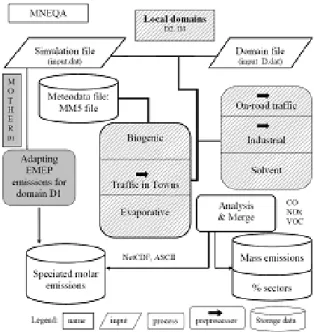
do-Figure 3. Flow diagram for MNEQA model. Grey is for modules
in the mother domain, D1. Shading identifies modules in local do-main and solid black arrows symbolize preprocessors. From Ortega et al. (2009).
main D2 are supplied by domain D1. The model is executed taking the first 24 h as spin-up time.
2.4 MNEQA Emission model
MNEQA is an emission model developed by the authors (Ortega et al., 2009). As it is a critical part of the air qual-ity modelling system, in this section we present a general overview and an outline of the differences in the methodol-ogy applied to D1 and D2 domains.
2.4.1 General overview
Nested domains are commonly applied to air quality modelling systems because the constituent meteorological, emission and photochemistry models must deal with grid variability and various domain ranges. As a result of the variability in spatial resolution, MNEQA methodology dif-fers from one domain to another. The main differences be-tween the domains are grid resolution and total range covered in one or more countries. Although the same degree of emis-sions description is desirable for all domains, information on emission sources and anthropogenic activities is not de-tailed enough or available in all jurisdictions. Nevertheless, the European Union has taken some action in this regard: it has developed the European Pollutant Emission Register (EPER http://eper.ec.europa.eu) for the reporting years 2001 and 2004, and the Pollutant Release and Transfer Registers (PRTR) for 2007.
Due to the difficulty in recording the data required by an emissions model for a very large domain, the
methodol-Table 1. Quantitative performance statistics for ozone concentration prediction, using 9 km grid domain.
Statistical parameter Mathematical definition
Mean bias (MB) M B = 1
N PN
1(Cm− C0)
Mean normalized bias error (MNBE) M N BE = 1 N PN 1 “ Cm−C0 C0 ” · 100%
Mean fractionalized bias (MFB) M F B = N1 PN 1 » Cm−C0 “Cm+C0 2 ” – · 100%
Mean absolute gross error (MAGE) M AGE = 1 N
PN
1 |Cm− C0|
Mean normalized gross error (MNGE) M N GE = 1 N PN 1 “|C m−C0| C0 ” · 100%
Normalized mean error (NME) N M E = PN
1|Cm−C0|
PN
1 C0 · 100%
Normalized mean bias (NMB) N M B = PN
1(Cm−C0)
PN
1 C0 · 100%
Root mean square error (RMSE) RM SE = q
1 N
PN
1 (Cm− C0)2
Unpaired peak prediction accuracy (UPA) U P A =Cm(max)−C0(max)
C0(max) · 100%
ogy applied in the mother domain (D1) is top-down, while that applied in the inner domain (D2) is mainly bottom-up. A modular structure was developed to take into ac-count the characteristics of every emission source. Figure 3 shows the MNEQA flow chart and its structure. The mod-ule for D1 adapts EMEP emissions (Vestreng et al., 2006) for time and space resolutions in D1. A simulation file provides general information about the simulation period to the D1 module and also to D2 (striped in Figure 3). Do-main files with the description of the grid of the doDo-main being simulated are fed to the modules. Some modules (such as: Biogenic, Traffic in Towns and Evaporative) re-quire a meteorological data file because the emissions de-pend on meteorological parameters such as temperature and radiation. Preprocessors (solid black arrows in Figure 3) are available for the following modules: Traffic in Towns, In-dustrial and On-road Traffic. Finally, the module Analy-sis and Merge creates outputs (in ASCII and NetCDF for-mats) from MNEQA simulations: speciated molar emis-sions, as required by CMAQ; mass emissions for CO, NOx and VOCs and particulate matter; and mass percentage of the contribution to total emissions from every emissions module.
MNEQA uses the output from a meteorological model to calculate temperature and radiation data. Finally, the com-pound emissions are classified into the species used in the photochemical mechanism: MNEQA does the speciation for CB-05.
2.4.2 Emissions in D1 domain
MNEQA uses a simple top-down methodology based on emissions data from the EMEP (May, 2007) expert emissions inventory (Vestreng et al., 2006). Europe and a small section of North Africa are covered by the EMEP domain, with a 50 × 50 km2 grid resolution. Emissions are computed from national data on 11 sectors, five main pollutants (CO, NH3, NMVOC, NOx, SOx) and two types of particulate matter (PM 2.5 and PM coarse). The available emissions data cover a period of several years. The algo-rithm consisted of assigning to each mother domain cell the emissions value of the nearest EMEP cell, multiplied by a proportional factor. This factor represents the ratio between the number of D1 cells and the number of EMEP domain cells intersecting within D1.
Speciation is computed using profiles from the California Air Resources Board (CARB) website (http://arb.ca.gov/ei/speciate/dnldopt.htm#specprof). Month-ly and weekMonth-ly profiles (Parra, 2004) have been applied to determine an emissions value for each hour based on the day of the week and the month of the year.
2.4.3 Emissions in D2 domain
In the case of the local domain, we have used a bottom-up approach for biogenic, traffic, residential consumption and industrial emissions. Taking various geometrical char-acteristics into account, we distinguished between surface, linear and point sources. These geometrical characteristics
Figure 4. Evolution, for the period studied, of the daily MB and RMSE. (a) (top left) corresponds to air temperature at 1.5 m (a.g.l.); (b)
(top right) corresponds to wind velocity measured at 10 m (a.g.l.) and (c) corresponds to wind direction measured at 10 m (a.g.l.).
are reflected in our calculations using a geographical infor-mation system (GIS). Finally, the emissions are merged for every grid cell because the photochemical model does not distinguish between the various types of sources; all that is required is one emissions value for each grid cell, each time step and each compound.
2.4.4 Air quality model configuration
In this section, the characteristics of the configuration used in the simulations performed with the air quality model are described. The domain D1 has a horizontal grid res-olution of 27 km and the inner domain, D2, 9 km. D1 has an extension of 68 × 44 grid cells centred at latitude 41.42◦N and longitude 1.40◦E. D2 has its bottom left corner at D1 (31, 19) with 30 × 30 grid cells. The total number of vertical model levels is 30 for all domains, up to 100 Pa. Because the photochemical model requires boundary data, the data domains have fewer cells at each horizontal bound-ary. For that reason, MNEQA and CMAQ are performed in D1 with 66 × 42 grid cells and in D2 with 28 × 28 grid
cells One-hour time step resolution is used in all domains and models.
3 Statistical air-quality model evaluations against measurements
As an air quality model is a conjunction of three models, meteorological, photochemical and emission, and since the latter has already been compared with other emission models (Ortega et al., 2009), in this section the results of the MM5 meteorological model and CMAQ photochemical model will be evaluated.
3.1 Evaluation of meteorological fields
Modelling results have been evaluated from a set of dif-ferent surface meteorological stations distributed over Cat-alonia belonging to the CatCat-alonia Meteorological Service. The evaluation includes wind velocity and wind direction measured at 10 m above ground level (a.g.l.) and air
tempera-Figure 5. Topographical features of the studied area and the
loca-tion of the 22 air-quality staloca-tions (•) used.
ture at 1.5 m (a.g.l.). The root mean square error (RMSE) and mean bias (MB) for these meteorological parameters have been calculated for hourly data provided by the model and observations (see Table 1 for definition), obtaining a daily statistical value. Wind statistics and wind direction are cal-culated for wind velocity higher than 0.5 m s−1, as wind di-rection is not reliable for lower velocities. The computation of statistical parameters is straightforward for wind veloc-ity and temperature, but the circular nature of wind direction makes it difficult to obtain the corresponding statistics. To avoid this problem we have used a modified wind direction, wherein 360◦was either added to or subtracted from the pre-dicted value to minimize the absolute difference between the observed and predicted wind directions (Lee and Fernando, 2004). For example, if the prediction is 10◦ and the corre-sponding observation is 340◦, then a predicted value of 370◦ is used.
Figure 4 shows the evolution of the RMSE and MB of the wind velocity, wind direction and temperature for the studied period. Wind speed (Figure 4a) points out an RMSE delimited between 1 and 3 m s−1 and an MB between 0 to 2 m s−1during most of the period, from May to the middle of September, from this point until the end of the period, RMSE increases to 4 m s−1and MB to 3.5 m s−1. The first period is mainly characterized by anticyclonic situation with small pressure gradients favouring the development of mesoscale circulations such as the sea breeze regime in the coast and mountain winds inland. Wind velocity associated with these circulation patterns is reproduced quite well by the model, although it tends to slightly underestimate wind velocity dur-ing the day and overestimate it at night. The model does not accurately reproduce very weak winds (Bravo et al., 2008),
Figure 6. Time evolution of averaged hourly ozone concentrations
provided by the air-quality model and the 48 air-quality stations for the studied period.
typical of the area studied at night. This causes the positive MB value during all period. During the second period, the meteorological situation has been much more variable led by synoptic scale given rise to higher MB and RMSE values.
Figure 4b shows the evolution of the RMSE and MB for wind direction. The RMSE ranges between 60◦to 120◦ for the first period, while during the second period limits vary between 80◦ and 140◦. MB values range from 20◦ to -20◦ with highest deviation during the second period.
The evolution of the RMSE and MB for air tempera-ture is presented in Figure 4c. For most of the period stud-ied, RMSE ranges between 3 and 4 degrees, while the MB ranges between -2 and -4 degrees. These values highlight the tendency to underestimate the air temperature at 1.5 m (a.g.l.).
The performance of the meteorological model agrees with several previous studies of meteorological applications for air quality modelling (Zhang et al., 2006a), especially those based on the area of study, (Jim´enez et al., 2008; Jim´enez et al., 2006a) where the classical statistics for sur-face fields have been reported (e.g., temperature, wind speed range from 1 to 4 degrees and 2 to 4 m s−1). However, our statistical evaluation shows a slightly greater dispersion, mainly for wind direction. The main reason could be the hor-izontal resolution, as meteorological studies over complex terrains require more horizontal and vertical resolution for resolving complex mesoscale circulation patterns (Jim´enez et al., 2006a).
3.2 Evaluation of the photochemical model
Statistical metrics for photochemical model perfor-mance assessment are calculated for surface ozone concen-trations at 48 measurement sites in the 9 × 9 km2 mod-elling domain. Although there is a newer guideline for
Table 2. Summary statistics corresponding to selected air quality stations associated with air-quality simulations of hourly and maximum
1-h and 8-h ozone average concentrations for the studied period.
Statistic Hourly averaged Hourly averaged for 1-h max. concentration 8-h max. concentration (00 to 24 UTC) ozone concentrations for ozone concentrations for ozone concentrations
≥ 60 µg m−3 ≥ 60 µg m−3 ≥ 60 µg m−3 MB (µg m−3) 1.35 -1.90 -2.34 -0.83 MAGE (µg m−3) 31.21 16.47 14.72 11.96 MNBE (%) 6.90 -0.41 0.11 1.12 MNGE (%) 41.98 19.95 14.66 13.31 MFB (%) -2.52 -4.61 -1.67 -0.48 RMSE (µg m−3) 29.97 21.75 19.38 16.10 NMB (%) 0.93 -2.21 -2.42 -1.00 NME (%) 21.52 19.18 15.22 14.48 UPA (%): 11.5
evaluating model performance, US EPA (2007), in this study we have used US EPA (2005), as the new guide-line does not include range quantification in the statisti-cal metrics. The three multi-site metrics used are the un-paired peak prediction peak accuracy (UPA), the mean nor-malized bias error (MNBE) and the mean nornor-malized gross error (MNGE). As well as the general guidance and proto-cols for air-quality performance evaluation (Seigneur et al., 2000), new statistical metrics based on the concept of fac-tors for overcoming the limitations of the traditional mea-surements are calculated. These statistics are summarized in Table 1.
For the evaluation, hourly measurements of ozone con-centration from 20 May to the end of October 2008 (here-after “studied period”) are reported by 48 air-quality surface stations named XVPCA (Xarxa de Vigil`ancia i Previsi´o de la Contaminaci´o Atmosf`erica) belonging to the Environmen-tal Department of the CaEnvironmen-talan Government This network of stations covers the size of the area with an accurate terri-torial distribution. However, given the grid cell resolution, 9 × 9 Km2, not all measurement stations satisfy the criterion for being representative of the area in which it is located. That is, if the grid cell is representative of a rural area, the measurement station cannot be located in the main town as its measurements will be representative of an urban area. Us-ing this criterion, the validation is performed with only 22 representative stations (see Figure 5 and Table 3).
In addition to the previous metrics, the US Environmen-tal Protection Agency (US EPA, 2005) developed a guideline indicating that it is inappropriate to establish a rigid crite-rion for model acceptance or rejection (i.e. no pass/fail test). However, building on past ozone modelling applications (US EPA, 1991) common values ranges for bias, error and accu-racy have been established. The accepted criteria are MNBE, ±5 to ±15%; MNGE, +30 to +35%; UPA ±15 to ±20%. For the entire period studied, the results in Table 2 show av-erages of the statistics metrics for hourly surface concentra-tions, daily peak 1-h values and daily peak 8-h ozone con-centrations.
For hourly averaged ozone concentrations, results in-dicate that the model shows a slight tendency to overesti-mate ground level ozone concentration (Table 2), as MB, MNBE and NMB values are positive, and although MNBE is within the EPA recommended performance goal of ±15%, the MNGE value is higher than the accepted criterion (35%). This behaviour of 24-h average ozone concentrations is prob-ably due to the excessive contribution of ozone concentra-tions during the night forecasted by the model.
The three main sources of error could be: (i) the model does not represent nocturnal physicochemical processes ac-curately enough (Jim´enez et al., 2006b); (ii) the emission model may not calculate night-time emissions properly; (iii) meteorological parameters, such as wind velocity, wind di-rection and vertical mixing are not well reproduced by the model when the synoptic forcing is weak and the ambient winds are light and variable (Sch¨urmann et al., 2009; Bravo et al., 2008).
As shown in Figure 6, the model overestimates ozone concentrations at night. To solve this problem, model eval-uation statistics are often calculated using only the hourly observation-prediction pairs for which the observed concen-tration is greater than a specific value. This procedure re-moves the influence of low concentrations, such as night-time values. Various cutoff values have been used for this purpose; however, 60 µg m−3 is frequently employed and is in accordance with EPA practice (US EPA, 1991; Sistla et al., 1996). When we apply this restriction, MNGE de-creases to 19.95%, which is below the EPA’s recommended performance goal of 35%, although the model tends to un-derestimate ozone mixing ratios, as MB, NMB, MFB and MNBE are -1.90 µg m−3, -2.21%, -4.61% and -0.41% re-spectively. For 1-h maximum concentration using the same restriction, the model tends to underestimate (albeit not in all 22 stations) the maximum value, as MB is -2.34 µg m−3, NMB is -2.42%, MFB is -1.67% and MNBE is 0.11%. In addition, MNGE is 14.66%, therefore all values are within the regulatory framework. For 8-h maximum concentra-tion, the model behaviour is similar as MB is -0.83 µg m−3,
Figure 7. Time evolution of averaged hourly ozone concentrations provided by the air-quality model and some selected air-quality stations
for the studied period.
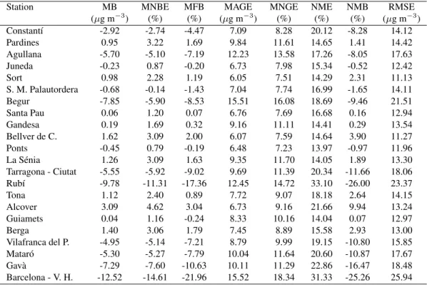
MNBE is 1.12%, NMB is -1.0%, MFB is -0.48% and MNGE is 13.31%. Small positive values for MNBE, correspond-ing to 1-h and 8-h maximum ozone concentrations, indicate that in some stations the ratio between modelled and ob-served ozone concentrations is slightly higher than the unity therefore, in these locations, the modelling system overesti-mates ozone concentrations. The UPA value calculated as the difference between the highest observed value and highest predicted value over all hours and monitoring stations over the entire period is 11.5%, which meets the EPA’s ±20% goal. In addition, if daily UPA values are calculated, re-sults indicate that almost all values of this statistic (81%) are well within the EPA criteria for an acceptable model per-formance. As a summary of Table 2 we conclude that the model shows a slight tendency to underestimate ozone con-centrations, as when we applied a reference threshold in or-der to avoid nocturnal values, some statistics become neg-ative. The information provided in Table 2 is extended to each monitoring station used in this study (Table 3). In ad-dition, some examples of time evolution of averaged hourly
ozone concentrations provided by the air-quality model and selected air-quality stations are presented in Figure 7. This additional information confirms the results and conclusion derived from Table 2. The performance of the photochemi-cal model agrees with several previous results on air quality modelling in the studied area, (Jim´enez et al., 2008; Jim´enez et al., 2006a), where statistical values also are within the EPA criteria.
As well as the statistical validation, unsystematic and systematic root mean square error, RMSEu(1) and RMSEs (2), are computed in order to evaluate the intrinsic error in the model and the random error (Appel et al., 2007).
RM SEu= v u u t 1 N N X i=1 (C − Cm)2 (1) RM SEs= v u u t 1 N N X i=1 (C − C0)2 (2)
Table 3. Statistics corresponding to selected air quality stations associated with air-quality simulations of hourly averaged for ozone
concentrations ≥ 60 µg m−3.
Station MB MNBE MFB MAGE MNGE NME NMB RMSE
(µg m−3) (%) (%) (µg m−3) (%) (%) (%) (µg m−3) Constant´ı -2.92 -2.74 -4.47 7.09 8.28 20.12 -8.28 14.12 Pardines 0.95 3.22 1.69 9.84 11.61 14.65 1.41 14.42 Agullana -5.70 -5.10 -7.19 12.23 13.58 17.26 -8.05 17.63 Juneda -0.23 0.87 -0.20 6.73 7.98 15.34 -0.52 12.42 Sort 0.98 2.28 1.19 6.05 7.51 14.29 2.31 11.13 S. M. Palautordera -0.68 -0.14 -1.43 7.04 7.74 16.99 -1.65 14.11 Begur -7.85 -5.90 -8.53 15.51 16.08 18.69 -9.46 21.51 Santa Pau 0.06 1.20 0.07 6.76 7.69 16.68 0.16 12.94 Gandesa 0.19 1.69 0.32 9.16 11.11 14.41 0.29 13.54 Bellver de C. 1.62 3.09 2.00 6.07 7.59 14.64 3.90 11.27 Ponts -0.45 0.79 -0.19 6.48 7.23 13.97 -0.97 11.96 La S´enia 1.26 3.09 1.63 9.35 11.70 14.05 1.89 13.30 Tarragona - Ciutat -5.55 -5.92 -9.02 9.69 11.39 20.34 -11.66 18.06 Rub´ı -9.78 -11.31 -17.36 12.45 14.72 33.10 -26.00 23.37 Tona 1.12 2.40 0.89 7.72 9.07 18.18 2.64 14.15 Alcover 3.09 4.62 3.04 6.73 9.16 21.66 9.94 13.24 Guiamets 0.04 1.16 -0.24 8.33 10.16 14.04 0.07 12.97 Berga 1.40 3.06 1.79 7.45 8.89 15.58 2.93 13.00 Vilafranca del P. -4.95 -5.14 -7.21 8.79 9.99 19.15 -10.80 15.85 Matar´o -5.30 -5.27 -7.79 10.04 11.64 20.60 -10.87 17.67 Gav`a -7.29 -7.60 -10.63 10.11 11.29 22.86 -16.47 18.48 Barcelona - V. H. -12.52 -14.61 -21.96 15.52 18.34 31.33 -25.26 25.94 C = a + bC0 (3) RM SEs= p (RM SEu)2+ (RM SEs)2 (4) Cmand C0values are modelled and observed concen-trations, respectively; a and b are the least-squares regres-sion coefficients derived from the linear regresregres-sion between Cmand C0; and N is the total number of model/observation pairs.
These new measurements help to identify the sources or types of error, which can be of considerable help in refining a model. The RMSEsrepresents the portion of the error that is attributable to systematic model errors; and the RMSEu rep-resents random errors in the model or model inputs that are less easily addressed. For a good model, the unsystematic portion of the RMSE must be much larger than the system-atic portion, whereas a high systemsystem-atic RMSEs value indi-cates a poor model.
Results are given in Tables 4 and 5 for each month an-alyzed (June-September 2008). May and October are not in-cluded, as the evaluation began on May 19 and twelve days are not representative, while during October there were sev-eral gaps.
For the case studied, results for 1-h and 8-h peak ozone concentrations show that systematic error values are lower than unsystematic ones, except for September and June, re-spectively. However, errors are similar, which implies that the air-quality system still has to be improved and refined. To analyze these results better, we should plan to carry out an
expanded detailed analysis identifying the key factors that in-fluence these prediction biases, such as sensitivity to synoptic conditions, to the boundary layer scheme used in the MM5 meteorological model, to the boundary conditions prescribed and to the chemical mechanisms used in CMAQ model. 3.3 Modelling quality objectives for ozone
“Uncer-tainty” defined by directive EC/2008/50
In 2008 a new European air quality directive was rati-fied by the European parliament (EC 2008). This directive replaced earlier directives with the intention of simplifying and streamlining reporting, as well as the introduction of new limit values concerning PM2.5. Whilst previous directives had based assessments and reporting largely on measurement data, this new directive places more emphasis on the use of models to assess air quality within zones and agglomerations. The increased focus on modelling allows the Member States more flexibility in reporting assessments and the potential to reduce the cost of air quality monitoring. However, mod-elling, like monitoring, requires expert implementation and interpretation. Models must also be verified and validated before they can be confidently used for air quality assess-ment or manageassess-ment (Denby et al., 2008).
The quality objectives for a model are given as a per-centage uncertainty. Uncertainty is then further defined in the directive as follows: ‘The uncertainty for modelling is defined as the maximum deviation of the measured and
cal-Table 4. Systematic and random errors for averaged 1-h peak ozone concentration. Month RMSEs(µg m−3) `RM SEs RM SE ´2 · 100 (%) RMSEu(µg m−3) RMSE (µg m−3) June 11.32 (28.32) 18.01 21.27 July 14.35 (45.30) 15.77 21.32 August 9.15 (24.67) 15.99 18.42 September 15.40 (54.86) 13.97 20.79
Table 5. Systematic and random errors for averaged 8-h peak ozone concentration.
Month RMSEs(µg m−3) `RM SEs RM SE ´2 · 100 (%) RMSEu(µg m−3) RMSE (µg m−3) June 16.54 (61.09) 13.20 21.16 July 11.99 (45.70) 13.07 17.74 August 10.48 (39.35) 13.01 16.71 September 12.64 (43.83) 14.31 19.09
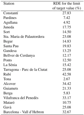
Table 6. RDE values calculated for the 22 representative stations
taken into account all studied period.
Station RDE for the limit of target value (%) Constant´ı 27.83 Pardines 7.42 Agullana 4.92 Juneda 17.75 Sort 14.50
Sta. Maria de Palautordera 23.08
Begur 14.83 Santa Pau 19.83 Gandesa 13.25 Bellver de Cerdanya 12.17 Ponts 12.50 La S´enia 15.42
Tarragona - Parc de la Ciutat 25.08
Rub´ı 42.58
Tona 2.67
Alcover 34.42
Guiamets 21.33
Berga 5.83
Vilafranca del Pened`es 33.17
Matar´o 10.75
Gav`a 25.08
Barcelona - Vall d’Hebron 32.67
culated concentration levels for 90% of individual monitor-ing points, over the period considered, by the limit value (or target value in the case of ozone), without taking into account the timing of the events. The uncertainty for modelling shall be interpreted as being applicable in the region of the ap-propriate limit value (or target value in the case of ozone). The fixed measurements that have to be selected for com-parison with modelling results shall be representative of the scale covered by the model.’
3.3.1 The mathematical formulation of the Directive’s quality objectives
As in the previous directives, the wording of this text remains ambiguous. Since values are to be calculated, a mathematical formula would have made the meaning much clearer. As such, the term ‘model uncertainty’ remains open to interpretation. Despite this, Denby et al. (2008) sug-gest that it should be called the Relative Directive Error (RDE) and define it mathematically at a single station as follows:
RDE = |OLV − MLV|
LV (5)
where OLV is the closest observed concentration to the limit value concentration or the target value for ozone and MLV is the correspondingly ranked modelled concentra-tion. The maximum of this value found at 90% of the avail-able stations is then the Maximum Relative Directive Error (MRDE).
For ozone, average RDE values calculated as a percent-age for the 22 representative stations are presented in Ta-ble 6. Results show a broad spread, ranging from low values (2.67%) in small towns to high values in cities and industri-alized areas where it is difficult to take all the emissions into account.
MRDE values, calculated as percentages for each month as well as for the whole period considered are presented in Table 7. As in the previous section, May and October are not included, as the evaluation began on May 19, and twelve days is considered not representative. During October there were several gaps.
MRDE values presented in Table 6 show percentages within the regulatory framework recommended in the Euro-pean Directive EC/2008/50, which is 50%.
Table 7. MRDE values for each month period as well as for all
period.
Month MRDE for the limit of target value (%)
June 34.42 July 31.33 August 27.83 September 33.50 All period 33.17 4 Conclusions
This paper describes the evaluation of a coupled regional modelling system used to simulate ozone air quality over the North-Western Mediterranean area (Catalonia) during late spring, summer and early autumn, 2008. The modelling system consists of the MM5 mesoscale model, the MNEQA emission model and the CMAQ photo-chemical model. Although the same meteorological and photochemical models have been applied in Catalonia in recent years, they have been evaluated during short periods and using a different emission model. This study has demonstrated the ability of the air quality modelling system MM5/MNEQA/CMAQ to forecast ozone concentrations with sufficient accuracy, as the statistics fell within the EPA and European recommended performance goals. Day-time results for average, 1-h and 8-h predictions indicate satisfactory behaviour of the model. However, modelled ozone concentrations at night are beyond measure and some statistics lie outside the regulatory framework. This behaviour of the model could be attributed to several factors, such as poor calculation of emissions at night, the failure to represent nocturnal physicochemical processes with sufficient accuracy, and finally, the inability of the model to reproduce certain meteorological parameters, such as wind velocity and wind direction at night. Results from systematic and unsystematic errors show similar values, although unsystematic errors tend to be slightly larger. In addition, although the model statistics are within the performance goals, some of these statistics, when calculated locally, do not meet regulatory targets. This evaluation also evinces a set of problems that need to be solved in future validations. The domain resolution over Catalonia must be improved, as air pollution dispersion studies in complex terrain require high resolution modelling of air quality in order to resolve complex circulation patterns like sea breezes, drainage flows or channelling flows, which are not always seen by the meteorological model using coarse horizontal resolution. In addition, by increasing resolution, a greater number of stations could be included in the validation. A new 3 km resolution is currently being introduced.
Acknowledgements. This research was supported by the Catalan Government under contracts FBG-304.471 and FBG-304.980. The authors gratefully acknowledge the technicians of this department for providing information about the emissions inventory and air-quality measurements. Thanks are extended to the Catalan Mete-orological Service for providing the initial and boundary meteoro-logical fields for executing MM5.
References
Abdul-Wahab, S. A., Bakheit, C. S., and Al-Alawi, S. M., 2005: Principal component and multiple regression analysis in mod-elling of ground-level ozone and factors affecting its concentra-tion, Environ Modell Softw, 20, 1263–1271.
Aguirre-Basurko, E., Ibarra-Berastegui, I., and Madariaga, I., 2006: Regression and multilayer perceptron-based models to forecast hourly O3 and NO2 levels in the Bilbao area, Environ Modell Softw, 21, 430–446.
Appel, K. W., Gilliland, A. B., Sarwar, G., and Gilliam, R. C., 2007: Evaluation of the Community Multiscale Air Quality (CMAQ) model version 4.5: Sensitivities impacting model performance. Part I-Ozone, Atmos Environ, 41, 9603–9615.
Brankov, E., Henry, R. F., Civerolo, K. L., Hao, W., Rao, S. T., Misra, P. K., Bloxam, R., and Reid, N., 2003: Assessing the ef-fects of transboundary ozone pollution between Ontario, Canada and New York, USA, Environ Pollut, 123, 403–411.
Bravo, M., Mira, T., Soler, M. R., and Cuxart, J., 2008: Intercom-parison and evaluation of MM5 and Meso-NH mesoscale models in the stable boundary layer, Bound-Layer Meteor, 128, 77–101. Byung, D. W. and Ching, J. K. S., 1999: Science algorithms of the EPA Models-3 Community Multiscale Air Quality (CMAQ) Modelling System, U.S. EPA/600/R-99/030.
Denby, B., Larssen, S., Guerreiro, C., Douros, J., Moussiopoulos, N., Fragkou, L., Gauss, M., Olesen, H., and Miranda, A. I., 2008: Guidance on the use of models for the European air quality di-rective, ETC/ACC Report.
Dudhia, J., 1996: A multi-layer soil temperature model for MM5. Preprints, Sixth PSU/NCAR Mesoscale Model Users’ Work-shop, NCAR, Boulder, CO, 49-50.
Dudhia, J., Gill, D., Manning, K., Wang, W., and Bruyere, C., 2004: PSU/ NCAR mesoscale modeling system tutorial class notes and user’s guide: MM5 modeling system version 3, NCAR, http:// www.mmm.ucar.edu/mm5/documents/tutorial-v3-notes.html. EMEP, 2007: EMEP/MMSC-W Technical Report 1/2006 ISSN
1504-6179, http://www.emep.int.
Gangoiti, G., Millan, M., Salvador, R., and Mantilla, E., 2001: Long-range transport and re-circulation of pollutants in the western Mediterranean during the project Regional Cycles of Air Pollution in the West-central Mediterranean Area, Atmos Envi-ron, 35, 6267–6276.
Grell, G., 1993: Prognostic evaluation of assumptions used by cu-mulus parameterizations, Mon Weather Rev, 121, 764–787. Grell, G., Dodhia, J., and Stauffer, D., 1994: A Description of the
Fifth Generation Penn State/ NCAR Mesoscale Model (MM5), NCAR. Tech. Note TN-398+STR, NCAR, Boulder, CO, 117 pp. Grossi, P., Thunis, P., Martilli, A., and Clappier, A., 2000: Effect of sea breeze on air pollution in the greater Athens area: Part II: Analysis of different Emissions Scenarios, J Appl Meteorol, 39, 563–575.
Guderian, R., Tingey, D. T., and Rabe, R., 1985: Effects of pho-tochemical oxidants on plants. Air Pollution by Phopho-tochemical Oxidants, Guderian R., Springer, Berlin, pp. 129-333.
Hewit, C., Lucas, P., Wellburn, A., and Fall, R., 1990: Chemistry of ozone damage to plants, Chem Ind, 15, 478–481.
Hogrefe, C., Rao, S. T., Kasibhatla, P., Kallos, G., Tremback, C. T., Hao, W., Sistla, G., Mathur, R., and McHenry, J., 2001: Evaluat-ing the performance of regional-scale photochemical modellEvaluat-ing systems: Part II- ozone predictions, Atmos Environ, 35, 4175– 4188.
Hurley, P. J., Physick, W. L., and Luhar, A. K., 2005: TAPM: a practical approach to prognostic meteorological and air pollu-tion modelling, Environ Modell Softw, 20, 737–752.
Jimenez, J., Baldasano, J. M., and Dabdub, D., 2003: Comparison of photochemical mechanisms for air quality modeling, Atmos Environ, 37, 4179–4194.
Jim´enez, P., Jorba, O., Parra, R., and Baldasano, J. M., 2006a: Eval-uation of MM5-EMICAT2000-CMAQ performance and sensitiv-ity in complex terrain: High-resolution application to the North-eastern Iberian Peninsula, Atmos Environ, 40, 5056–5072. Jim´enez, P., Lelieveld, J., and Baldasano, J. M., 2006b:
Multi-scale Modelling of air pollutants Dynamics in the North-Western Mediterranean Basin during a typical summertime episode, J Geophys Res, 111, D18 306.
Jim´enez, P., Jorba, O., Baldasano, J. M., and Gass´o, S., 2008: The Use of a Modelling System as a Tool for Air Quality Manage-ment: Annual High-Resolution Simulations and Evaluation, Sci Total Environ, 390, 323–340.
Lee, S. and Fernando, H. J. S., 2004: Evaluation of Meteorolog-ical Models MM5 and HOTMAC Using PAFEX-I Data, J Appl Meteorol, 43, 1133–1148.
Mauzerall, D. L., Sultan, B., Kim, J., and Bradford, D., 2005: NOx emissions: variability in ozone production, resulting health dam-ages and economic costs, Atmos Environ, 39, 2851–2866. Millan, M., Mantilla, E., Salvador, R., Carratala, A., Sainz, J. M.,
Alonso, L., Gangoiti, G., and Navazo, M., 2000: Ozone cycles in the western Mediterranean basin: Interpretation of monitoring data in complex coastal terrain, J Appl Meteorol, 39, 487–508. Ortega, S., Soler, M. R., Alarc´on, M., and Arasa, R., 2009:
MNEQA: An emissions model for photochemical simulations, Atmos Environ, 43, 3670–3681.
Parra, R., 2004: Desarrollo del modelo EMICAT2000 para la es-timaci´on de emisiones de contaminantes del aire en Catalu˜na y su uso en modelos de dispersi´on fotoqu´ımica, PhD Dissertation, Universitat Polit`ecnica de Catalunya, Spain, PhD Dissertation, http://www.tdx.cat/TDX-0803104-102139.
San Jos´e, R., Stohl, A., Karatzas, K., Bohler, T., James, P., and P´erez, J. L., 2005: A modelling study of an extraordinary night time ozone episode over Madrid domain, Environ Modell Softw, 20, 587–593.
Schlink, U., Herbarth, O., Richter, M., Dorling, S., Nunnari, G., Gawley, G., and Pelikan, E., 2006: Statistical models to assess the health effects and to forecast ground level ozone, Environ Modell Softw, 21, 547–558.
Schultz, P., 1995: An explicit cloud physics parameterization for op-erational numerical weather prediction, Mon Weather Rev, 123, 3331–3343.
Sch¨urmann, G. J., Algieri, A., Hedgecock, I. M., Manna, G., Pir-rone, N., and Sprovieri, F., 2009: Modelling local and syn-optic scale influences on ozone concentrations in a topograph-ically complex region of Southern Italy, Atmos Environ, 43,
4424–4434.
Seigneur, C., Pun, B., Pai, P., Louis, J. F., Solomon, P., Emery, C., Morris, R., Zahniser, M., Worsnop, D., Koutrakis, P., White, W., and Tombach, I., 2000: Guidance for the performance evaluation of three-dimensional air quality modeling systems for particulate matter and visibility, J Air Waste Manage Assoc, 50, 588–599. Serrano, E., Macias, A., and Castro, M., 1993: An improved direct
method of rubber craking analysis for estimating 24-hour ozone levels, Atmos Environ, 27, 431–442.
Silibello, C., Calori, G., Brusasca, G., Catenacci, G., and Finzi, G., 1998: Application of a photochemical grid model to Milan metropolitan area, Atmos Environ, 32, 2025–2038.
Sistla, G., Zhou, N., Hao, W., Ku, J. Y., and Rao, S. T., 1996: Ef-fects of uncertainties in meteorological inputs of Urban Airshed Model predictions and ozone control strategies, Atmos Environ, 30, 2011–2025.
Sitch, S., Cox, P. M., Collins, W. J., and Huntingford, C., 2007: Indirect Radiative Forcing of Climate Change through Ozone Ef-fects on the Land-Carbon Sink, Nature, 448, 791–794.
Sokhi, R. S., San Jos´e, R., Kitwiroon, N., Fragkou, E., P´erez, J. L., and Middleton, D. R., 2006: Prediction of ozone levels in London using the MM5-CMAQ modelling system, Environ Modell Softw, 21, 566–576.
Soler, M. R., Hinojosa, J., Bravo, M., Pino, D., and Vil`a Guerau de Arellano, J., 2004: Analyzing the basic features of different com-plex terrain flows by means of a Doppler Sodar and a numerical model: Some implications to air pollution problems, Meteorol Atmos Phys, 85, 141–154.
Troen, I. S. and Mahrt, L., 1986: A simple model of the atmospheric boundary layer; sensitivity to surface evaporation, Bound-Layer Meteor, 37, 129–148.
US EPA, 1991: Guideline for Regulatory Application of the Ur-ban Airshed Model, Office of Air and Radiation, Office of Air Quality Planning and Standards, Technical Support Division, Re-search Triangle Park, North Carolina, US, US EPA Report No. EPA-450/4-91-013.
US EPA, 2005: Guidance on the use of models and other analy-ses in attainment demonstrations for the 8-hour ozone NAAQS, Office of Air Quality Planning and Standards, Research Triangle Park, North Carolina, US, US EPA Report No. EPA-454/R-05-002. October 2005, 128 pp.
US EPA, 2007: Guidance of the use of models and other analysis for demonstrating attainment of air quality goals for ozone, PM2.5 and Regional haze, US Environmental protection Agency, Re-search Triangle Park, North Carolina, US, EPA-454/B-07-002. Vestreng, V., Rigler, E., Adams, M., Kindbom, K., Pacyna, J. M.,
Denier van der Gon, H., Reis, S., and Travnikov, O., 2006: In-ventory review. Emission data reported to LRTAP and NEC Di-rective; Stage 1, 2, and 3 review; Evaluation of inventories of HMs and POPs.
Yarwood, G., Roa, S., Yocke, M., and Whitten, G., 2005: Updates to the carbon bond chemical mechanism: CB05, Final report to the US EPA, RT-0400675, http://www.camx.com.
Zhang, Y., Liu, P., Pun, B., and Seigneur, C., 2006a: A Compre-hensive Performance Evaluation of MM5-CMAQ for the Summer 1999 Southern Oxidants Study Episode, Part-I. Evaluation Pro-tocols, Databases and Meteorological Predictions, Atmos Envi-ron, 40, 4825–4838.
Zhang, Y., Liu, P., Queen, A., Misenis, C., Pun, B., Seigneur, C., and Wu, S. Y., 2006b: A Comprehensive Performance Evaluation of MM5-CMAQ for the Summer 1999 Southern Oxidants Study
Episode, Part-II.Gas and Aerosol Predictions, Atmos Environ, 40, 4839–4855.
Zunckel, M., Koosailee, A., Yarwood, G., Maure, G., Venjonoka, K., van Tienhoven, A. M., and Otter, L., 2006: Modelled surface ozone over southern Africa during the Cross Border Air Pollution Impact Assessment Project, Environ Modell Softw, 21, 911–924.