Università degli Studi di Napoli Federico II
DOTTORATO DI RICERCA IN
FISICA
Ciclo XXXI
Coordinatore: prof. Salvatore Capozziello
Investigating the three-dimensional architecture
of genomes by polymer physics
Settore Scientifico Disciplinare FIS/02
Dottorando
Tutore
Carlo Annunziatella
Prof.
Mario Nicodemi
I
Contents
Introduction
1. Three-Dimensional organization of the genome
1.1. The genome in the cell nucleus
1.2. Epigenetics and gene regulation
1.3. Chromosome Conformation Capture and further technologies
1.3.1. 3C-based techniques: 3C, 4C and 5C
1.3.2. Hi-C technique
1.3.3. Ligation independent methods: GAM and SPRITE
1.3.4. FISH technique
1.4. Nuclear organization of chromatin
1.4.1. Chromatin loops
1.4.2. A/B compartments
1.4.3. Topologically Associated Domains
1.4.4. Besides TADs: the meta-TADs structures
1.4.5. Interpretation of the structural data and further information
2. 3D chromatin investigation by polymer physics models
2.1. String&Binders Switch (SBS) Model and its implementation by MD
simulation
2.1.1. The SBS model
2.1.2. The MD potentials
2.1.3. Langevin equation
2.1.4. Lennard-Jones dimensionless units
2.1.5. Preparation of the initial configurations
2.2. Phase diagram and structural characterization
2.2.1. Phase diagram and order parameter
2.2.2. Pairwise and multi-way contacts
II
2.2.4. Folding dynamics
2.3. Fitting experimental data
2.4. Self-interacting domains and hierarchical organization
3. Modeling real loci by polymer physics
3.1. Generalization of the SBS model: PRISMR method
3.2. Modeling real loci
3.2.1. Methods for Molecular Dynamics simulations
3.2.2. HoxB locus
3.2.3. Sox9 locus and molecular nature of the binding domains
3.3. Impact of 3-dimensional changes in cell regulation
3.3.1. Structural changes of the HoxD locus at different stages of differentiation
3.3.2. SBS model of the HoxD locus
3.3.3. Investigating HoxD genes locus at single-cell level
3.3.4. High-multiplicity regulatory contacts
3.4. Investigating tissue-specific interactions by 3D modeling
3.4.1. Emerging scenario from cHi-C data
3.4.2. Three-dimensional investigation of Pitx1 landscape by 3D modeling
4.
Predicting Structural Variants effects on chromatin architecture
4.1.
Epha4 locus: studied datasets
4.2. PRISMR models of the murine Epha4 locus
4.2.1. Statistical significance and robustness of identified binding domains
4.2.2. Epigenomic barcoding of PRISMR binding domains in the EPHA4 locus
4.2.3. The ‘PRISMR + CTCF’ method
4.2.4. Computational details
4.3. PRISMR Model predictions on mouse cells
4.3.1. 3D conformations of the polymer models of the Epha4 locus and its
mutations
4.3.2. Statistical analysis details
4.4. PRISMR Model predictions on human cells
Conclusions
III
Acknowledgments
Appendices
A. Comparing different chromatin polymer models
A. 1.
The Loop Extrusion Model
A. 2.
The Diffusive Loop Extrusion Model
A. 3.
The String&Binders Switch
pag. 1
Introduction
In mammalian cell nuclei, chromosomes have a spatial organization that is strictly related to cellular biological functions, such as regulation of gene transcription and expression (Bickmore and Van Steensel, 2013; Dekker et al., 2013; Lieberman-Aiden et al., 2009; Misteli, 2007; Tanay and Cavalli, 2013). However, still today, the three-dimensional organization of genome and the mechanisms driving its folding are not completely known and represent an open question in modern biology. In recent years, new technologies have been developed to help to investigate, for the first time, the genome architecture in a quantitative way. These methods, such as Chromosome Conformation Capture (3C) techniques, measure the interaction frequencies between pairs of genomic regions across a cell population (Dekker et al., 2013). In particular, they have revealed that the genome is characterized by a complex non-random structure, that occurs at different genomic length scales through the formation of many local and long-range interactions (Beagrie et al., 2017; Lieberman-Aiden et al., 2009; Quinodoz et al., 2018). In the nucleus, chromosomes occupy distinct territories, whose preferred positions depend on cell type and transcription activity (Bickmore and Van Steensel, 2013; Misteli, 2007; Tanay and Cavalli, 2013). Within each chromosome, the genome is organized in self-interacting domains, called “topologically associated domains” (briefly, TADs) (Dixon et al., 2012; Nora et al., 2012), in which chromatin regions frequently interact with each other. Such domains are approximately 0.5-1 Mb long and result to be highly conserved across species, cell lines and tissue types (Dixon et al., 2012; Fraser et al., 2015; Nora et al., 2012; Phillips-Cremins et al., 2013; Sexton et al., 2012). At a higher order level TADs, in turn, interact with each other giving rise to a hierarchy of domains-within-domains, called meta-TADs, extending up to chromosomal scales (Fraser et al., 2015). This 3D architecture of chromatin has key functional roles, as for instance to control gene activity through the formation of physical loops between regulatory regions and target remote genes. The disruption of such an intricate network of interactions can alter the regular gene activity and produce effects directly on the phenotype (Lupiáñez et al., 2015; Spielmann and Mundlos, 2013).
To make sense of genome-wide contact data, and to explain the principles shaping chromosome 3D structure, models from polymer physics have been recently introduced (Barbieri et al., 2012; Brackley et al., 2016; Chiariello et al., 2016; Fudenberg et al., 2016; Giorgetti et al., 2014; Jost et al., 2014; Marenduzzo et al., 2006; Nicodemi and Prisco, 2009; R. K. Sachs, G. Van Den Engh, B. Trask, H.
pag. 2
Yokota, 1995; Rosa and Everaers, 2008; Sanborn et al., 2015; Tiana et al., 2016). This is an innovative and fascinating research field at the confluence of physics and biology.
In this framework, the research presented in my Ph.D. thesis has been developed. It has been conducted under the supervision of Professor Mario Nicodemi, in the group of Complex Systems at the Physics Department of the University of Naples “Federico II”. Many results have been published or are currently under development in collaboration with the Epigenetic Regulation and Chromatin Architecture group directed by Prof. Ana Pombo, at Max Delbruck Centre For Molecular Medicine (Berlin), and the Development and Disease Group directed by Professor Stefan Mundlos, at the Max Planck Institute for Molecular Genetics (Berlin).
The thesis is organized in four principal chapters and one Chapter of Appendices. In Chapter 1, we highlight the importance of genome spatial organization and we briefly recall some basic concepts from biology, needed for the comprehension of this research activity, as the Chromosome Conformation Capture (3C) techniques, the interpretation of genome interaction data and the relationship between spatial organization and cell functionality. In Chapter 2, we describe a polymer physics model developed in our group to make sense of the complex pattern of genomic interactions and to explain, in a quantitative way the interaction network emerging from Hi-C contact data. In particular, we show that scaling concepts of classical polymer physics explain the large-scale behavior of contact data over three orders of magnitudes in genomic separation, across different cell types and chromosomes; we present a theoretical study of the multiple co-localization contact landscape and, finally, we schematically model the mechanisms underlying the self-assembly of topological domains. In Chapter 3, we introduce a more complex polymer physics model, by which we can reconstruct, with good accuracy, the 3D organization of real genomic regions. Finally, in Chapter 4, we test if such polymer model predicts the effect on chromatin architecture of structural variants (SVs), such as deletions, duplication or inversion. We show how polymer modeling emerges, in this scenario, as a valid approach for predicting pathogenic effects, facilitating the interpretation and diagnosis of this type of genomic rearrangements. In Appendix A, we show a direct comparison of different polymer physics models, which have shown to have an important role in explaining chromatin spatial organization.
pag. 3
References
Barbieri, M., Chotalia, M., Fraser, J., Lavitas, L.-M., Dostie, J., Pombo, A., and Nicodemi, M. (2012). Complexity of chromatin folding is captured by the strings and binders switch model. Proc. Natl. Acad. Sci. 109, 16173–16178.
Beagrie, R.A., Scialdone, A., Schueler, M., Kraemer, D.C.A., Chotalia, M., Xie, S.Q., Barbieri, M., De Santiago, I., Lavitas, L.M., Branco, M.R., et al. (2017). Complex multi-enhancer contacts captured by genome architecture mapping. Nature 543, 519–524.
Bickmore, W.A., and Van Steensel, B. (2013). Genome architecture: Domain organization of interphase chromosomes. Cell 152, 1270–1284.
Brackley, C.A., Johnson, J., Kelly, S., Cook, P.R., and Marenduzzo, D. (2016). Simulated binding of transcription factors to active and inactive regions folds human chromosomes into loops, rosettes and topological domains. Nucleic Acids Res. 44, 3503–3512.
Chiariello, A.M., Annunziatella, C., Bianco, S., Esposito, A., and Nicodemi, M. (2016). Polymer physics of chromosome large-scale 3D organisation. Sci. Rep. 6.
Dekker, J., Marti-Renom, M.A., and Mirny, L.A. (2013). Exploring the three-dimensional organization of genomes: Interpreting chromatin interaction data. Nat. Rev. Genet. 14, 390–403. Dixon, J.R., Selvaraj, S., Yue, F., Kim, A., Li, Y., Shen, Y., Hu, M., Liu, J.S., and Ren, B. (2012). Topological domains in mammalian genomes identified by analysis of chromatin interactions. Nature
485, 376–380.
Fraser, J., Ferrai, C., Chiariello, A.M., Schueler, M., Rito, T., Laudanno, G., Barbieri, M., Moore, B.L., Kraemer, D.C., Aitken, S., et al. (2015). Hierarchical folding and reorganization of chromosomes are linked to transcriptional changes in cellular differentiation. Mol. Syst. Biol. 11, 852–852.
Fudenberg, G., Imakaev, M., Lu, C., Goloborodko, A., Abdennur, N., and Mirny, L.A. (2016). Formation of Chromosomal Domains by Loop Extrusion. Cell Rep. 15, 2038–2049.
Giorgetti, L., Galupa, R., Nora, E.P., Piolot, T., Lam, F., Dekker, J., Tiana, G., and Heard, E. (2014). Predictive polymer modeling reveals coupled fluctuations in chromosome conformation and transcription. Cell 157, 950–963.
Jost, D., Carrivain, P., Cavalli, G., and Vaillant, C. (2014). Modeling epigenome folding: Formation and dynamics of topologically associated chromatin domains. Nucleic Acids Res. 42, 9553–9561. Lieberman-Aiden, E., Van Berkum, N.L., Williams, L., Imakaev, M., Ragoczy, T., Telling, A., Amit, I., Lajoie, B.R., Sabo, P.J., Dorschner, M.O., et al. (2009). Comprehensive mapping of long-range interactions reveals folding principles of the human genome. Science (80-. ). 326, 289–293.
Lupiáñez, D.G., Kraft, K., Heinrich, V., Krawitz, P., Brancati, F., Klopocki, E., Horn, D., Kayserili, H., Opitz, J.M., Laxova, R., et al. (2015). Disruptions of topological chromatin domains cause pathogenic rewiring of gene-enhancer interactions. Cell 161, 1012–1025.
pag. 4
Biophys. J. 90, 3712–3721.
Misteli, T. (2007). Beyond the Sequence: Cellular Organization of Genome Function. Cell 128, 787– 800.
Nicodemi, M., and Prisco, A. (2009). Thermodynamic pathways to genome spatial organization in the cell nucleus. Biophys. J. 96, 2168–2177.
Nora, E.P., Lajoie, B.R., Schulz, E.G., Giorgetti, L., Okamoto, I., Servant, N., Piolot, T., Van Berkum, N.L., Meisig, J., Sedat, J., et al. (2012). Spatial partitioning of the regulatory landscape of the X-inactivation centre. Nature 485, 381–385.
Phillips-Cremins, J.E., Sauria, M.E.G., Sanyal, A., Gerasimova, T.I., Lajoie, B.R., Bell, J.S.K., Ong, C.T., Hookway, T.A., Guo, C., Sun, Y., et al. (2013). Architectural protein subclasses shape 3D organization of genomes during lineage commitment. Cell 153, 1281–1295.
Quinodoz, S.A., Ollikainen, N., Tabak, B., Palla, A., Schmidt, J.M., Detmar, E., Lai, M.M., Shishkin, A.A., Bhat, P., Takei, Y., et al. (2018). Higher-Order Inter-chromosomal Hubs Shape 3D Genome Organization in the Nucleus. Cell 219683.
R. K. Sachs, G. Van Den Engh, B. Trask, H. Yokota, and J.E.H. (1995). A random-walk / giant-loop model for interphase chromosomes. Proc. Natl. Acad. Sci. USA 92, 2710–2714.
Rosa, A., and Everaers, R. (2008). Structure and dynamics of interphase chromosomes. PLoS Comput. Biol. 4.
Sanborn, A.L., Rao, S.S.P., Huang, S.-C., Durand, N.C., Huntley, M.H., Jewett, A.I., Bochkov, I.D., Chinnappan, D., Cutkosky, A., Li, J., et al. (2015). Chromatin extrusion explains key features of loop and domain formation in wild-type and engineered genomes. Proc. Natl. Acad. Sci. 112, E6456– E6465.
Sexton, T., Yaffe, E., Kenigsberg, E., Bantignies, F., Leblanc, B., Hoichman, M., Parrinello, H., Tanay, A., and Cavalli, G. (2012). Three-dimensional folding and functional organization principles of the Drosophila genome. Cell 148, 458–472.
Spielmann, M., and Mundlos, S. (2013). Structural variations, the regulatory landscape of the genome and their alteration in human disease. BioEssays 35, 533–543.
Tanay, A., and Cavalli, G. (2013). Chromosomal domains: Epigenetic contexts and functional implications of genomic compartmentalization. Curr. Opin. Genet. Dev. 23, 197–203.
Tiana, G., Amitai, A., Pollex, T., Piolot, T., Holcman, D., Heard, E., and Giorgetti, L. (2016). Structural Fluctuations of the Chromatin Fiber within Topologically Associating Domains. Biophys. J. 110, 1234–1245.
pag. 5
Chapter 1: Three-Dimensional organization of the
genome
The spatial architecture of the genome in the nucleus of eukaryotic cells is the principal way by which cells regulate their biological functions, such as transcription and regulation of gene expression. Although the link between 3D genome architecture and regulation of cellular functions is still not completely known, novel experimental protocols have been developed in the last years, and are still now, to investigate deeply and in a more quantitative way this open question.
In this first chapter, we briefly give an overall overview of the genome architecture problem, introducing the most important results achieved during the last decade in this research field, and the experimental methods that made possible to obtain them. This will help the comprehension of our research activity, described in more detail in the following chapters. In Section 1.1 and Section 1.2, we summarize some fundamental concepts of molecular biology and recent advances about gene regulation and epigenetics. In Section 1.3, we introduce the fundamental technologies which have allowed to investigate the spatial organization of genomes. Finally, in Section 1.4, we summarize important findings obtained from the analysis of interactions data, provided by the described experimental technologies, and we briefly discuss the scenario that is now emerging, also thanks to the help of polymer physics models.
The results described in this chapter have been introduced and discussed in the papers from (Dekker et al., 2013; Dixon et al., 2012; Fraser et al., 2015; Lieberman-Aiden et al., 2009; Lupiáñez et al., 2015; Nora et al., 2012; Rao et al., 2014).
1.1 The genome in the cell nucleus
DNA (deoxyribonucleic acid) is a molecule carrying all genetic instructions needed for the cell development. DNA is a double helix of two chains, each made of monomer units, called nucleotides, bound to one another in the chain filament by covalent bonds. A nucleotide is composed of a sugar called deoxyribose, a phosphate group and one of four nitrogen-containing nucleobases, that are cytosine (C), guanine (G), adenine (A) or thymine (T). For making the double-stranded DNA, the nitrogenous bases of the two chains are bound together by hydrogen bonds, according to base pairing rules: A with T and C with G. The sequence of these four nucleobases encodes the genetic information. The DNA strand has a directionality that is defined by the orientation of the 3′ and 5′
pag. 6
carbons along the sugar-phosphate backbone. The two strands of double-helix structure run in opposite directions to each other and are thus antiparallel.
In the nucleus of the eukaryotic cells, the DNA is always associated with a variety of proteins, called histones, whose principal function is to package the DNA filament in a more compact way. Histones have also further functions, such as to control the gene expression, to prevent DNA damages and drive the DNA replication. The complexity of the chromatin packing allows, for instance, to include the entire mammalian genome, which would have a linear length of about 2 meters, into a nucleus of roughly 5÷15 μm diameter. The complex made of DNA and proteins is called chromatin. The basic units of the chromatin packing are the nucleosomes. Each nucleosome consists of a structure of eight histone proteins (consisting of two copies of each histone H2A, H2B, H3 and H4) and of 1.7 times wrapped DNA of approximately 146 base pairs (bps).
At a higher level, the chromatin is organized in chromosomes, each one restricted in a specific region, called chromosomal territory (CT), clearly visible using microscopy techniques, as shown in Figure 1.1 (Cremer and Cremer, 2001). The total length of genome, which depends on the number of chromosomes and on the number of copies for each chromosome (named ploidy), varies across the different species. For instance, the human cells, as well as the most part of the eukaryotic cells, have two different copies per chromosome (diploid cells) and 23 different chromosomes, amounting to 6.4x10⁹ base pairs. Each chromosome contains several hundreds of thousands of nucleosomes, and
each nucleosome is separated from the next one by a filament of linker DNA, long up to about 80 bps. When viewed by microscopy, chromosomes assume the appearance of a string of beads where the beads are nucleosomes and string is the linker DNA.
Figure 1.1: Chromosomes territory organization.
Microscopy image of the nucleus of chicken cell showing the organization of chromosomes in distinct regions, called chromosomal territories (CTs), each colored in a different way. Within the chromosomes, the chromatin at lower scale has a very complex three-dimensional organization, strictly related on gene expression of cells. However, this structure is still unknown and represent an open problem in modern biology. Figure adapted from (Cremer and Cremer, 2001).
pag. 7
Within the nucleus, the chromatin is found in two different structural forms, which play an important role in gene expression: heterochromatin and euchromatin. These forms were distinguished from the the different degree of compaction of “beads on a string” structure. Heterochromatin is a condensed form of chromatin, where nucleosomes are tightly packed, by making the DNA hardly accessible to the polymerase and therefore lowly transcribed. It is usually localized to the periphery, near the nuclear lamina. On the other hand, the euchromatin, that is the most part of the genome (up to 90%), is lightly packed DNA and is characterized by a high level of transcription.
1.2 Epigenetics and gene regulation
In a multicellular organism, all the cells share the same genome. Each specific cell line in the organism expresses a subset of all genes making up the genome of the species. During cellular differentiation, i.e., the process where a cell passes from one cell type to another, a change from one pattern of gene expression to another occurs. The transcriptional activity of a gene is regulated by a genomic region (long about 100/1000 bases), located near the transcription start site (TSS) of the gene, named promoter. Promoters provide an initial binding site for the transcriptional machine, including RNA polymerase and transcription factors. The gene activity can also be controlled by additional regulatory regions of DNA, named enhancers, which increase the probability of gene transcription. Enhancers have a key role in driving cell type-specific gene expression, and they can activate transcription of their target genes at great genomic distances, ranging from several hundreds, until to even thousands of bases (Bulger and Groudine, 2011; Calo and Wysocka, 2013; Ong and Corces, 2011; Phillips-Cremins et al., 2013).
By the term “epigenetics”, we indicate all the features that affect the gene activity and its expression, without involving changes in genome sequence. Examples of mechanisms that produce such changes are DNA methylation and histone modification, each of which alters how genes are expressed without altering the underlying DNA sequence. Additionally, the gene expression can be controlled through the action of repressor proteins that attach to silencer regions of the DNA. In last years, new technologies have been developed to analyze genome-wide epigenetic modifications at base-pair resolution. Among these, chromatin immunoprecipitation followed by next-generation sequencing (ChIP-seq), a method that allows to identify the binding site along the DNA associated with a specific protein, by using specific antibodies that target the protein of interest. Such techniques allow to identify some consistent patterns of histone marks, used for example to better define DNA regulatory regions (Allis and Jenuwein, 2016).
pag. 8
1.3 Chromosomes Conformation Capture and further technologies
As discussed in the previous Sections, the three-dimensional organization of the chromatin has a key role in regulation of gene expression. It consists, indeed, of a complex network of contacts between genes and its corresponding regulatory elements, which allows the genes to be expressed or silenced. In the following Sections, we briefly describe two different molecular approaches that have been developed in last years to study the three-dimensional folding of chromosomes with increasing accuracy. On one side, the new genome-wide methods that allow to estimate the mean frequency of contact for any pairs of genomic regions. In particular, we focus on the methods based on the chromosome conformation capture (3C) technique. In this approach, two loci are considered in contact if their physical distance is close enough to become crosslinked (typically, around 100nm). On the other side, the FISH technique, an independent and conceptually different method, which enables to estimate the physical distances between a limited number of genomic regions at single cell level. Since that such information are not accessible with 3C-based methods, and a direct comparison is not trivial, they can be powerfully combined to bring comprehensive insights into genome folding.1.3.1 3C-based techniques: 3C, 4C and 5C
In last decade, several experimental techniques have been developed to deeply investigate the three-dimensional organization of chromatin in mammalian cell nucleus. These approaches are based on chromosome conformation capture (3C) technique and allow to estimate the frequency of interaction, across a population of cells, between different genomic regions, which could be physically close even if separated by several nucleotides along the linear genome. Such interactions have a key role in gene expression during cellular differentiation, as, for instance, to drive the interaction between enhancer and promoter (see, Section 1.2).
Figure 1.2: Chromosome conformation capture techniques.
Schematic representation of experimental steps that characterize the 3C methods. First (Step I), the chromatin is crosslinked with formaldehyde to create covalent bond between pairs of loci spatially close. Next, they are fragmented (Step II), ligated (Step III) and finally purified (Step IV). Figure adapted from (Dekker et al., 2013).
pag. 9
All 3C-based methods are characterized by following steps (schematically shown in Figure 1.2): I) Chromatin in nucleus is cross-linked by formaldehyde, generating covalent bonds
between different genomic regions which are physically close in the space;
II) By using restriction enzymes (e.g., HindIII, NcoI) during a digestion process, cross-linked chromatin is fragmented;
III) Cross-linked fragments are ligated to form a unique DNA molecule; IV) DNA is purified and pairwise interactions are quantified,
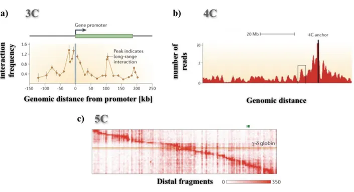
The 3C (Dekker et al., 2002) and 4C (Simonis et al., 2006) techniques detect the interactions involving a specific genomic region. The 3C method identifies the interactions for a single pair of loci and can be used to test a candidate of interacting pair, e.g. enhancer-promoter (Figure 1.3, Panel a).
Figure 1.3: Comparison of output for different 3C-based techniques.
a) Example of Chromosome Conformation Capture (3C) data. The horizontal axis indicates the genomic distance from the anchor point, or point of view, here indicated by a grey line. b) Example of 4C data, where the anchor point is indicated, by a black line. c) Example of 5C interaction data for the ENCODE ENm009 region in K562 cells. Here, each row represents the interaction profile of a transcription start site (TSS) across the 1 Mb region on human chromosome 11 that contains the beta-globin locus. Figures adapted from (Dekker et al., 2013).
pag. 10
On the other hand, the 4C technique allows to quantify the interaction profile of a given locus with all the surrounding genomic regions (Figure 1.3, Panel b). This not requires the a-priori knowledge of both interacting loci. Finally, by 5C method (Dostie et al., 2006) instead, we can detect the interactions between all the pairs of loci within a given genomic region, which typically is no longer than a single mega-base (Figure 1.3, Panel c)
1.3.2 Hi-C technique
The Hi-C method was the first genome-wide extension of 3C techniques, which made possible to detect long-range interactions (Lieberman-Aiden et al., 2009). In this approach, once the cells are fixed by formaldehyde (binding the interacting regions by covalent cross-link), fragmented and ligated (as discussed in Section 1.2.1), the staggered DNA ends are filled in with biotinylated nucleotides. In this way, it results a genome-wide collection of ligation products, corresponding to pairs of chromatin fragments that were spatially close in the nucleus. Each of these ligation products is marked with biotin at ligation junction. The library is then sheared, and the junctions are pulled down from biotin. The purified junctions are then directly sequenced along the genome, generating a list of interacting fragments. Finally, the genome is divided into windows of fixed length, which defines the Hi-C data resolution (Figure 1.4). The resolution depends on depth of sequencing and on data quality: in the first experiments the resolution was 1 Mb but recent Hi-C or Hi-C-derived, e.g. in situ Hi-C (Rao et al., 2014) or cHi-C (Jäger et al., 2015), experiments can reach 1 kb of resolution.
Figure 1.4: Hi-C method description.
Schematic representation of the Hi-C method protocol. The biotinylated junctions allow to efficiently detect the ligated fragments genome-wide. Figure adapted from (Lieberman-Aiden et al., 2009).
The Hi-C data are organized in contact matrices, where each bin xij represents the frequency of contact
pag. 11
xij is equal to xji, and the contact matrix is symmetrical. Since Hi-C is able to detect loci belonging to
the same chromosome or to different chromosomes, in the first case we say cis- data and the associated matrix is squared by definition, while in the second one we say trans- data. In our work, we focus on cis- data (as for example in Figure 1.5, Panel a). Fixed a given genomic window (for instance, the entire chromosome), the size of contact matrix depends on data resolution: higher is the resolution, bigger is the size of contact matrix.
Importantly, in Hi-C contact matrix, a bin xij represents the interaction frequency averaged over a
large population of cells. However, chromatin conformations, which are determined by several different factors, can have three-dimensional structures highly variable. Recently, single-cell Hi-C (scHi-C) technologies have been developed to investigate at single-cell level the 3D architecture of chromatin (Nagano et al., 2013; Stevens et al., 2017), revealing a high cell-to-cell variability. Such new methods provide a new approach to investigate these biological processes.
1.3.3 Ligation independent methods: GAM and SPRITE
As discussed in Section 1.2.1, the 3C methods developed to investigate genome-wide contacts are based on proximity ligation, which creates covalent bonds between regions spatially close. However, these technologies often fail to detect chromatin regions too far apart to directly ligate, although it has been proved that they have an important role in genome organization, as for example the nuclear bodies (Quinodoz et al., 2018). For this reason, two alternative ligation-free methods have been recently developed for more comprehensively understanding genome organization: Genome Mapping Architecture (GAM) and Split-Pool Recognition of Interactions by Tag Extension (SPRITE). Besides, these new approaches have made possible to investigate, besides pairwise interactions, also multi-way contacts, such as triplets, quadruplets, etc., which can help to shed light on the complexity of genome organization.
GAM (Beagrie et al., 2017) was the first genome-wide technology which allows to detect interactions between pairs of loci, without ligation process. Starting from a collection of slices obtained cryo-sectioning a population of nuclei in random directions, it is possible to estimate the frequencies of interaction between pairs of loci. The new idea is that two loci, which are frequently co-segregated in the same slice, will be also physically close in three-dimensional space (what would be not expected if the loci were independent and associated randomly). GAM technique summarizes the same results for interacting pairs found by Hi-C and, additionally, allows to investigate also multi-way contacts, helping to investigate the complex pattern of interactions characterizing genome organization. Furthermore, GAM enables the investigation of 3-d genome conformations at
single-pag. 12
cell level. To facilitate the comparison among these different techniques, an example of GAM contact matrix is shown in Figure 1.5, Panel b, for the same genomic region considered for Hi-C case.
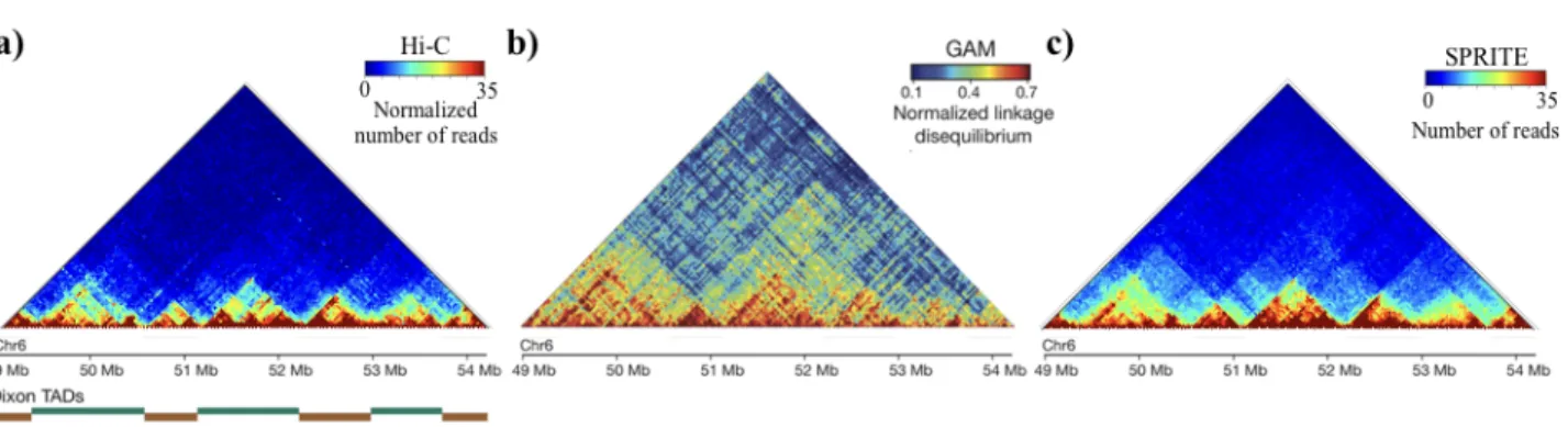
Figure 1.5: Comparison of average contact matrix from three different technologies.
Contact matrices from Hi-C, GAM and SPRITE technologies, for a genomic region on chromosome 6 (49 - 54.2 Mb) in mouse embryonic stem cells: a) Hi-C contact matrix from (Dixon et al., 2012). On bottom, we reported the TADs positions. b) Example of GAM matrix, where instead of co-segregation matrix, is reported the normalized linkage disequilibrium. The matrix shows a similar interaction pattern and an enrichment of long-range contact. Figure adapted (Beagrie et al., 2017). c) SPRITE matrix shows a pattern similar to those shown in Hi-C and GAM. (Quinodoz et al., 2018)
On the other hand, SPRITE (Quinodoz et al., 2018) is more similar approach to 3C-based methods, but it does not use the ligation process as well. After that chromatin is crosslinked and fragmented, the interacting molecules in a cluster are barcoded by using a split-pool strategy. Interactions are identified by sequencing and matching all the reads having the same barcode. The cluster obtained in this way are then converted in contact frequencies by counting all the contacts observed in a single cluster and weighting each contact by the total number of the molecules contained within the cluster. An example of contact matrix from SPRITE is shown in Figure 1.5, Panel c.
1.3.4 FISH technique
Fluorescent in situ hybridization (FISH) is a molecular technique that enables the measurement of physical distance between two target loci at single cell level, as it also allows to quantify the distribution of these distances across a cell population (Jefferson and Volpi, 2010). In FISH method, fluorescent probes bind target that can then be directly visualized using fluorescence microscopy, enabling its localization to be assessed in the context of the overall nuclear architecture and/or with respect to other genomic loci. Then, by indicating two targeted loci a and b, it is possible to estimate the associated probability distribution P(rab) measuring the variation of distance rab across the cell
pag. 13
population. Notably, this type of measure allows us to quantify the degree of variability of physical distances between pairs of genomic loci (Figure 1.6).
Figure 1.6: FISH experiments.
Starting from a population of cells, FISH method enables the measurement of cell-to-cell variability in distance rab between two genomic loci a and b. Indeed, the knowledge of probability distribution
of distances P(rab) allows, for instance, to compute the mean (and median) distance, or the fraction
of cells for which the distance rab is smaller than a certain threshold R. Figure adapted from (Giorgetti
and Heard, 2016).
1.4 Nuclear organization of chromatin
By analyzing 5C and Hi-C data, some fundamental features of chromatin structure were discovered. In the following Sections we summary the most important findings achieved in this field during the last years.
1.4.1 Chromatin loops
A chromatin loop event occurs when two genomic regions on the same chromosome (in cis-), are brought close in physical space. This mechanism allows to bring together in 3-d space two regions that could be event apart along the chromosome. It is biologically driven by a number of architectural proteins, such as cohesin, transcription factor, etc. and represents the fundamental mechanism driving gene activation, since chromatin loops can be formed between gene promoter with one (or more than one) enhancer region, even if located up to 1Mb away from the gene (downstream or upstream from TSS position). As discussed in Section 1.2, the physical proximity between the gene and its enhancers increases the probability that transcription of the gene could occur. In human genome, about one-half of genes are involved in long-range chromatin loops.
Physical interactions have been also detected between regions falling on different chromosomes. Although they are not loops in a narrow sense of the term, these interactions show similar features. However, the exact mechanism of loops formation in not still understood.
pag. 14
1.4.2 A/B compartments
Through the principal component analysis (PCA) of Hi-C contact matrices (Lieberman-Aiden et al., 2009), and consequently confirmed by independent FISH experiments, it was discovered that the entire genome could be divided into two different classes of regions, named “A” and “B” compartments. Genomic regions in the same compartment tend to interact preferentially with regions belonging to the same compartment, rather than to regions associated with the other compartment (Figure 1.7, Panel a).
Figure 1.7: Compartments A/B and TADs organization of the genome.
a) On left, an example of genome-wide Hi-C contact matrix for chromosome 14 from a karyotypically normal human lymphoblastoid cell line. On right, the Pearson correlation matrix of the same chromosome, and the principal component associated analysis. This last panel shows that PC correlates the checked pattern in matrix, which respectively defines A (positive values) and B compartment (negative values). b) Schematic cartoon showing TAD organization of chromosomes in the cell nucleus. Genomic regions within the same TAD interact each other much more frequently than regions belonging to a different TAD. TADs are separated by genomic region, called “boundary”. c) Comparison of Hi-C matrix over a systemic region for mouse (top) and human (bottom) stem cell, and corresponding TADs positions. The TADs are highly conserved across the different species. Figures adapted from (Dixon et al., 2012; Lieberman-Aiden et al., 2009).
A/B compartment-associated regions have typical size of some Mb (5÷10) and correlate with eu- and hetero-chromatin respectively (Section 1.1). While the A compartment tends to be less compact and
pag. 15
enriched of genes, correlating with higher expression and accessible chromatin, the B compartment, instead, tends to be more compact and gene-poor, with higher interaction values. The presence of A/B compartments is in full agreement with the known presence of open and closed chromatin in the cell nucleus.
1.4.3 Topologically Associated Domains
Besides the A/B compartments, chromatin shows a lower level of structural organization. Recent findings have shown that genome is organized in self-interacting domains (Dixon et al., 2012), called in literature Topologically Associating Domains (TADs) (Nora et al., 2012). The principal feature of TADs is that regions within a domain interact most frequently with regions within the same domain, rather than regions outside it (schematic cartoon in Figure 1.7, Panel b). Typically, TADs have size of about 0.5÷1 Mb (then smaller than the A/B compartments) and they are formed through the interaction of architectural proteins with DNA, which gives rise to several chromatin loops within it. TADs strictly correlate with regulation of gene expression, since they can be associated with active or inactive transcription and are almost conserved between different species (Figure 1.7, Panel c). As both mouse and human are composed by more than 2000 domains, covering almost all the genome, TADs are found to be universal building blocks of chromosomes. In Hi-C contact matrix, a TAD appears as a square along the principal diagonal, characterized by high interaction level of interaction (Figure 1.6, Panel a bottom). By using this observation, different computational algorithms have been developed to identify TADs from experimental data (Dixon et al., 2012; Fraser et al., 2015; Oluwadare and Cheng, 2017; Rao et al., 2014).
TADs represent physically isolated units along the genome, characterized by two distinct functional features: the regulation of genes within them, that allows chromatin interaction among loci within the same domain, and the separation of gene activity of two neighbouring TADs. Recent studies have shown that deletion of TAD boundary can lead to ectopic expression of several developmental regulator genes during limb formation, and to several congenital diseases. However, the mechanism that regulates the formation of TADs is still not clear, and several polymer models have been developed to help to quantitatively describe them (Barbieri et al., 2012; Bianco et al., 2018; Brackley et al., 2017; Chiariello et al., 2016; Fudenberg et al., 2016; Sanborn et al., 2015). Some of them (Brackley et al., 2017; Fudenberg et al., 2016; Sanborn et al., 2015) are based on observed enrichment of CTCF binding proteins at TAD boundaries (Rao et al., 2014), proving that CTCF is an important insulating factor in mammalian cell. However, such models do not take into account other possible factors, that have an important role in the formation of these domains (Barbieri et al., 2017; Dixon et al., 2016; Kundu et al., 2018; Yan et al., 2017).
pag. 16
1.4.4 Besides TADs: the meta-TADs structures
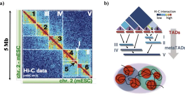
In the previous sections, we showed that chromosomes are organized in megabase-sized self-interacting domains, named TADs, which are arranged at a higher order level in A/B compartments, i.e., in nuclear domains enriched of active or repressed chromatin states. However, this scenario is too simplistic to efficiently explain the complex pattern of interactions found in the Hi-C data. As visible from data (Figure 1.8, Panel a), TADs (indicated by Arabic numbers) in turn, interact with each other at higher-order level of interaction, giving rise to a hierarchical structure of domains-within-domains, called meta-TADs (Latin number), extending across genomic scale up to the entire chromosome length (Fraser et al., 2015). This structure can be well investigated, whatever the cell type (human or mouse), by a tree-like structure (Figure 1.8, Panel b). The meta-TADs organization has been proved to correlate with several epigenomic features, and its changes during cell differentiation correlate with transcriptional state of the cell. Therefore, these hierarchical structures seem to have an important role in chromatin compaction and help the chromatin to re-organize itself and to activate or silence a specific genomic region, according to transcriptional state of the cell.
Figure 1.8: Meta-TAD structure.
a) Contact matrix Hi-C of chromosome 2 (53-58 Mb) from mouse embryonic stem cell, where we indicate the TADs by Arabic number. How appears clearly in the matrix, TADs, in turn, can interact with each other giving rise to higher order structures, the meta-TADs, that are here indicated by Latin numbers. b) Starting from matrix Hi-C, meta-TAD can be identified by single‐linkage clustering. Figures adapted from (Fraser et al., 2015).
pag. 17
Within TADs, in turn, there are smaller interacting domains, generally called “sub-TADs” (Phillips-Cremins et al., 2013; Rao et al., 2014). They seem to have similar features of TADs, but, on the contrary, they consistently differ across different cell lines. Even in this case, cell-type specific organization of sub-TADs appears to be related to cell-type specific regulatory events, as for instance, driving the activation of a gene (Figure 1.9).
Figure 1.9: TADs and sub-TADs organization.
Boundary regions (in brief, “boundary”) separating two TADs, are generally enriched in architectural proteins, such as transcriptional repressor CTCF. Hi-C data at high resolution have revealed the existence of lower level of chromatin organization, such as sub-TADs, which are smaller spatial domains (around 100 kb) that display a more dynamic nature and tissue specificity. Both TADs and sub-TADs can be schematized as loops, sometimes associated with enhancer-promoter interaction; they are bound by mediators and the cohesin complexes, displaying a dynamic and tissue-specific nature. The CTCF–cohesin complex proteins play a key part in the looping process, which explains some of the features observed in Hi-C interaction map. Figures adapted from (Spielmann et al., 2018).
1.4.5 Interpretation of the structural data and further information
Spatial proximity between different genomic regions can be the result of specific contacts mediated by protein complexes bridging them, or co-proximity near the same nuclear structure (i.e., nucleolus, nuclear lamina, etc.). All the experimental methods we described in previous Section 1.3, give information about the relative frequency of contact across a population of cells between pairs of loci. However, these do not give information about specificity of contacts; indeed, they do not distinguish the functional associations from non-functional ones, that could be caused by random collisions between different genomic regions, and made possible by chromatin flexibility. Similarly, they cannot even individuate what are the mechanisms driving the chromatin folding, that are still completely unknown.
pag. 18
Figure 1.10: Boundary deletion causes a TAD disruption in Epha4.
a) In the schematic representation of the wild-type genomic locus, gene A is expressed in the developing brain and gene B in the developing limbs. Both genes are regulated by their own tissue-specific cis-regulatory elements (red and blue, respectively) located in different TADs separated by boundary elements. b) An inter-TAD deletion of a boundary element can cause TAD fusion and enhancer adoption; the relocation of enhancer elements into a neighbouring TAD causes mis-expression and disease. Through the deletion of the boundary, the enhancer of gene B (blue) is free to act on gene A, driving ectopic expression in the developing limbs. Figures adapted from (Spielmann et al., 2018).
In order to shed light on these mechanisms of chromatin organization and to investigate the impact on health of its structural alteration, more and more experiments have been recently performing (Franke et al., 2016; Lupiáñez et al., 2015; Spielmann et al., 2018). These research activities have found that structural variations, such as duplications or deletions, involving even little genomic regions can be pathogenic and they often cause of congenital diseases (as shown, for instance, in Figure 1.10). Additionally, they have proved that high levels of structural variations are linked to human cancer genome. These results prove how chromatin organization in space and phenotype are very closely related, and the knowledge of mechanisms by which that structure is regulated is fundamental to prevent and recover congenital diseases. In the following chapter, we show how, by polymer physics approach, is possible to predict the effect of 3D spatial organization, due to structural variations, using as input information the data available for healthy subjects.
pag. 19
References
Allis, C.D., and Jenuwein, T. (2016). The molecular hallmarks of epigenetic control. Nat. Rev. Genet.
17, 487–500.
Barbieri, M., Chotalia, M., Fraser, J., Lavitas, L.-M., Dostie, J., Pombo, A., and Nicodemi, M. (2012). Complexity of chromatin folding is captured by the strings and binders switch model. Proc. Natl. Acad. Sci. 109, 16173–16178.
Barbieri, M., Xie, S.Q., Torlai Triglia, E., Chiariello, A.M., Bianco, S., De Santiago, I., Branco, M.R., Rueda, D., Nicodemi, M., and Pombo, A. (2017). Active and poised promoter states drive folding of the extended HoxB locus in mouse embryonic stem cells. Nat. Struct. Mol. Biol. 24, 515–524. Beagrie, R.A., Scialdone, A., Schueler, M., Kraemer, D.C.A., Chotalia, M., Xie, S.Q., Barbieri, M., De Santiago, I., Lavitas, L.M., Branco, M.R., et al. (2017). Complex multi-enhancer contacts captured by genome architecture mapping. Nature 543, 519–524.
Bianco, S., Lupiáñez, D.G., Chiariello, A.M., Annunziatella, C., Kraft, K., Schöpflin, R., Wittler, L., Andrey, G., Vingron, M., Pombo, A., et al. (2018). Polymer physics predicts the effects of structural variants on chromatin architecture. Nat. Genet. 50, 662–667.
Brackley, C.A., Johnson, J., Michieletto, D., Morozov, A.N., Nicodemi, M., Cook, P.R., and Marenduzzo, D. (2017). Nonequilibrium Chromosome Looping via Molecular Slip Links. Phys. Rev. Lett. 119.
Bulger, M., and Groudine, M. (2011). Functional and mechanistic diversity of distal transcription enhancers. Cell 144, 327–339.
Calo, E., and Wysocka, J. (2013). Modification of Enhancer Chromatin: What, How, and Why? Mol. Cell 49, 825–837.
Chiariello, A.M., Annunziatella, C., Bianco, S., Esposito, A., and Nicodemi, M. (2016). Polymer physics of chromosome large-scale 3D organisation. Sci. Rep. 6.
Cremer, T., and Cremer, C. (2001). Chromosome territories, nuclear architecture and gene regulation in mammalian cells. Nat. Rev. Genet. 2, 292–301.
Dekker, J., Rippe, K., Dekker, M., and Kleckner, N. (2002). Capturing chromosome conformation. Science (80-. ). 295, 1306–1311.
Dekker, J., Marti-Renom, M.A., and Mirny, L.A. (2013). Exploring the three-dimensional organization of genomes: Interpreting chromatin interaction data. Nat. Rev. Genet. 14, 390–403. Dixon, J.R., Selvaraj, S., Yue, F., Kim, A., Li, Y., Shen, Y., Hu, M., Liu, J.S., and Ren, B. (2012). Topological domains in mammalian genomes identified by analysis of chromatin interactions. Nature
485, 376–380.
Dixon, J.R., Gorkin, D.U., and Ren, B. (2016). Chromatin Domains: The Unit of Chromosome Organization. Mol. Cell 62, 668–680.
pag. 20
Krumm, A., Lamb, J., Nusbaum, C., et al. (2006). Chromosome Conformation Capture Carbon Copy (5C): A massively parallel solution for mapping interactions between genomic elements. Genome Res. 16, 1299–1309.
Franke, M., Ibrahim, D.M., Andrey, G., Schwarzer, W., Heinrich, V., Sch�pflin, R., Kraft, K., Kempfer, R., Jerković, I., Chan, W.L., et al. (2016). Formation of new chromatin domains determines pathogenicity of genomic duplications. Nature 538, 265–269.
Fraser, J., Ferrai, C., Chiariello, A.M., Schueler, M., Rito, T., Laudanno, G., Barbieri, M., Moore, B.L., Kraemer, D.C., Aitken, S., et al. (2015). Hierarchical folding and reorganization of chromosomes are linked to transcriptional changes in cellular differentiation. Mol. Syst. Biol. 11, 852–852.
Fudenberg, G., Imakaev, M., Lu, C., Goloborodko, A., Abdennur, N., and Mirny, L.A. (2016). Formation of Chromosomal Domains by Loop Extrusion. Cell Rep. 15, 2038–2049.
Giorgetti, L., and Heard, E. (2016). Closing the loop: 3C versus DNA FISH. Genome Biol. 17. Jäger, R., Migliorini, G., Henrion, M., Kandaswamy, R., Speedy, H.E., Heindl, A., Whiffin, N., Carnicer, M.J., Broome, L., Dryden, N., et al. (2015). Capture Hi-C identifies the chromatin interactome of colorectal cancer risk loci. Nat. Commun. 6.
Jefferson, A., and Volpi, E. V. (2010). Fluorescence in situ Hybridization (FISH) for Genomic Investigations in Rat (Humana Press, Totowa, NJ).
Kundu, S., Ji, F., Sunwoo, H., Jain, G., Lee, J.T., Sadreyev, R.I., Dekker, J., and Kingston, R.E. (2018). Erratum: Polycomb Repressive Complex 1 Generates Discrete Compacted Domains that Change during Differentiation (Molecular Cell (2017) 65(3) (432–446.e5) (S1097276517300357) (10.1016/j.molcel.2017.01.009)). Mol. Cell 71, 191.
Lieberman-Aiden, E., Van Berkum, N.L., Williams, L., Imakaev, M., Ragoczy, T., Telling, A., Amit, I., Lajoie, B.R., Sabo, P.J., Dorschner, M.O., et al. (2009). Comprehensive mapping of long-range interactions reveals folding principles of the human genome. Science (80-. ). 326, 289–293.
Lupiáñez, D.G., Kraft, K., Heinrich, V., Krawitz, P., Brancati, F., Klopocki, E., Horn, D., Kayserili, H., Opitz, J.M., Laxova, R., et al. (2015). Disruptions of topological chromatin domains cause pathogenic rewiring of gene-enhancer interactions. Cell 161, 1012–1025.
Nagano, T., Lubling, Y., Stevens, T.J., Schoenfelder, S., Yaffe, E., Dean, W., Laue, E.D., Tanay, A., and Fraser, P. (2013). Single-cell Hi-C reveals cell-to-cell variability in chromosome structure. Nature 502, 59–64.
Nora, E.P., Lajoie, B.R., Schulz, E.G., Giorgetti, L., Okamoto, I., Servant, N., Piolot, T., Van Berkum, N.L., Meisig, J., Sedat, J., et al. (2012). Spatial partitioning of the regulatory landscape of the X-inactivation centre. Nature 485, 381–385.
Oluwadare, O., and Cheng, J. (2017). ClusterTAD: An unsupervised machine learning approach to detecting topologically associated domains of chromosomes from Hi-C data. BMC Bioinformatics
18.
Ong, C.-T., and Corces, V.G. (2011). Enhancer function: new insights into the regulation of tissue-specific gene expression. Nat. Rev. Genet. 12, 283–293.
pag. 21
Phillips-Cremins, J.E., Sauria, M.E.G., Sanyal, A., Gerasimova, T.I., Lajoie, B.R., Bell, J.S.K., Ong, C.T., Hookway, T.A., Guo, C., Sun, Y., et al. (2013). Architectural protein subclasses shape 3D organization of genomes during lineage commitment. Cell 153, 1281–1295.
Quinodoz, S.A., Ollikainen, N., Tabak, B., Palla, A., Schmidt, J.M., Detmar, E., Lai, M.M., Shishkin, A.A., Bhat, P., Takei, Y., et al. (2018). Higher-Order Inter-chromosomal Hubs Shape 3D Genome Organization in the Nucleus. Cell 219683.
Rao, S.S.P., Huntley, M.H., Durand, N.C., Stamenova, E.K., Bochkov, I.D., Robinson, J.T., Sanborn, A.L., Machol, I., Omer, A.D., Lander, E.S., et al. (2014). A 3D map of the human genome at kilobase resolution reveals principles of chromatin looping. Cell 159, 1665–1680.
Sanborn, A.L., Rao, S.S.P., Huang, S.-C., Durand, N.C., Huntley, M.H., Jewett, A.I., Bochkov, I.D., Chinnappan, D., Cutkosky, A., Li, J., et al. (2015). Chromatin extrusion explains key features of loop and domain formation in wild-type and engineered genomes. Proc. Natl. Acad. Sci. 112, E6456– E6465.
Simonis, M., Klous, P., Splinter, E., Moshkin, Y., Willemsen, R., De Wit, E., Van Steensel, B., and De Laat, W. (2006). Nuclear organization of active and inactive chromatin domains uncovered by chromosome conformation capture-on-chip (4C). Nat. Genet. 38, 1348–1354.
Spielmann, M., Lupiáñez, D.G., and Mundlos, S. (2018). Structural variation in the 3D genome. Nat. Rev. Genet. 19, 453–467.
Stevens, T.J., Lando, D., Basu, S., Atkinson, L.P., Cao, Y., Lee, S.F., Leeb, M., Wohlfahrt, K.J., Boucher, W., O’Shaughnessy-Kirwan, A., et al. (2017). 3D structures of individual mammalian genomes studied by single-cell Hi-C. Nature 544, 59–64.
Yan, J., Chen, S.-A.A., Local, A., Liu, T., Qiu, Y., Lee, A.-Y., Jung, I., Preissl, S., Rivera, C.M., Wang, C., et al. (2017). Histone H3 Lysine 4 methyltransferases MLL3 and MLL4 Modulate Long-range Chromatin Interactions at Enhancers. BioRxiv 110239.
pag. 22
Chapter 2: 3D chromatin investigation by polymer
physics models
In the previous Chapter, we described the complex architecture of the chromatin in the nucleus of cells. To make sense of genome-wide contact data and to expose the principles shaping three-dimensional structure of chromosomes, several theoretical models have been developed from polymer physics. For the sake of completeness, we briefly describe some of these models, recently proposed, which have had a key role in quantitatively explaining the spatial organization of chromosomes.
Initially, as a possible structure of chromatin in the nucleus, the Fractal Globule model was proposed (van Berkum et al., 2010; Lieberman-Aiden et al., 2009; Mirny, 2011). Here, a compact polymer not-equilibrium state emerges during polymer condensation due to topological constrains and prevents one genomic region to pass across another one. This model was independently introduced in (Grosberg et al., 1988), but experimental evidences in biology were not found until the Hi-C paper (Lieberman-Aiden et al., 2009). Shorty later, another model was introduced, named Dynamic Loop model (Bohn and Heermann, 2010), where chromatin moves under diffusional motion and functional loops can be formed when two specific sites co-localize, thanks to the presence of mediating proteins, such as CTCF or transcription factors (TFs). These loops can be formed with a certain probability, and dissolve after a certain lifetime. Another important model, introduced in (Jost et al., 2014), tries to link structural and epigenetic information: starting from 1D epigenetic data, it is possible to associate to each chromatin region a specific epigenetic state. This model can explain TADs formation by introducing a specific interaction between regions characterized by the same epigenetic state. A similar approach has been later used to explain chromatin folding at chromosomal scales (Di Pierro et al., 2016). At the moment, however, two chromatin models are mainly considered: the String&Binders Switch (SBS) model (Nicodemi and Prisco 2009; Barbieri et al. 2012), that was also used in other independent studies (Brackley et al., 2013), and the Loop Extrusion (Fudenberg et al., 2016; Sanborn et al., 2015), together with the Slip-Link model (Brackley et al., 2017).
In this Chapter, we will focus on the SBS model, which is having an important role in genome 3-dimensional reconstruction and that we will use in more detail in this and the following Chapters for our considerations about chromatin architecture. In Section 2.1, we describe the SBS model, as introduced in (Barbieri et al., 2012; Nicodemi and Prisco, 2009), and how we implemented it for the
pag. 23
first time by using a Molecular Dynamics (MD) approach. In Section 2.2, we will discuss the resulting phase diagram for the polymer model, which shows novel thermodynamic stable states. In Section 2.3 and Section 2.4, we show how, just using few parameters, besides recapitulating the average behaviour of chromatin folding at chromosomal scales, we are able to explain by the SBS model the formation of interacting domains and the hierarchical organization of higher-order structures of chromatin.
Most of the results shown in this chapter, including figures, paragraphs and sentences, is adapted or lifted verbatim from the following papers, which I co-authored: (Annunziatella et al., 2016, 2018, Chiariello et al., 2016, 2017).
2.1 String & Binders Switch (SBS) Model and its implementation by
MD simulations
In the following Section, we describe in detail the SBS model (Barbieri et al., 2012; Nicodemi and Prisco, 2009) and how we implement it by a Molecular Dynamics (MD) approach, which is widely used in the computational community to investigate such models of chromatin. In the MD approach, the trajectory of each particle in the system is determined by numerically solving its equations of motion (e.g., by Verlet algorithm); the interaction with the other particles are taken into account by introducing appropriate potentials. Unlike the Monte-Carlo method, used, e.g., in (Barbieri et al., 2012), the MD approach allows to investigate not only the equilibrium properties of the system but also its dynamics. Our simulations are run via LAMMPS (Large-scale Atomic/Molecular Massively Parallel Simulator) (Plimpton, 1995), a MD program that is optimized for parallel computing, allowing to drop significantly the time of simulations.
2.1.1 The SBS model
In the String&Binders Switch (SBS) model, a chromatin filament (we call the “string”) is represented as a self-avoiding walk (SAW) polymer chain made of consecutive beads. The beads interact with diffusing molecules (the “binders”), in solution at a given concentration c, which can bring two beads in physical proximity and loop the polymer. The scale of such interaction is indicated by Eint. The
interaction between binders and polymer beads drives the folding of the chain. Different equilibrium thermodynamics phases exist according to the value of the control parameters, Eint and c, giving rise
to specific, corresponding conformational classes. A schematic cartoon of the SBS model is represented in Figure 2.1, Panel a, in the simplest case with only one type of binders and binding sites (red); yet, to describe more complex situations, different types of beads (and cognate binders)
pag. 24
can be introduced, schematically represented by different “colours”. (Annunziatella et al., 2016; Barbieri et al., 2012, 2017; Bianco et al., 2018; Chiariello et al., 2016)
Figure 2.1: String&Binders Switch (SBS) polymer model describing chromatin folding. a) In the String&Binders Switch (SBS) model chromatin folding is driven by the interactions between the polymer chain of beads (the ‘string’) and the binding molecules (called ‘binders'). b) Interaction potential between consecutive beads making up the polymer chain. This is a combination of repulsive Lennard-Jones potential (VIJ, blue dashed line) and FENE potential (VFENE, yellow dashed line). Here,
we set ε=1, σ=1, R0=1.6σ and kFENE = 30kBT/σ2. c) Attractive potential between chain bead and cognate
binders Vint(r), modeled by a truncated-shifted LJ potential. The absolute value of the minimum of
Vint(r) defines the scale of interaction energy, Eint (horizontal dashed line in figure), Here, we set
εint=12kBT, σbb= 1σ, and rint= 1.5σ. Figures adapted from (Annunziatella et al., 2018; Chiariello et al.,
2016).
2.1.2 The MD potentials
In our MD simulations, the SAW polymer chain is composed by N consecutive beads, having each a diameter σ. To model hard-core repulsion and prevent physical overlap among particles, between any two beads i and j we introduce a truncated Lennard-Jones (LJ) potential VLJ, described by the
following expression: VLJ=! 4ε "# σ rij$ 12 -#rσ ij$ 6 % +ε r&'<2σ1/6 0 otherwise (2.1)
pag. 25
where σ is the diameter of a bead, rij = |ri-rj| is the center-to-center distance and ε = kBT the strength
of the potential (T temperature of the system and kB Boltzmann constant). This is a continuous
decreasing positive function of rij that becomes zero for rij =21/6σ, as shown in Figure 2.1, Panel b
(blue curve). Excluded volume effects between beads are taken into account by such term, which drastically hampers physical overlaps between beads.
To model the bond between two consecutive beads in the chain, an established approach (Kremer and Grest, 1990) considers that between any pair of consecutive beads there is the finitely extensible
nonlinear elastic (FENE) potential VFENE:
VFENE=-kFENER0 2 2 ln(1- ) |ri+1-ri| R0 * 2 + (2.2)
where ri and ri+1 are the position of neighboring bead on polymer, kFENE is the strength of the FENE
spring and R0 is its maximal extension. The FENE potential is close to a harmonic potential for values
of the distance r=|ri+1-ri| near to zero (r ⟶0) and diverges for r ⟶R0, which represent the maximal
length of the bond (Figure 2.1, Panel b, yellow curve).
The resulting total potential, V(r) = VLJ +VFENE (shown in Figure 2.1, Panel b, green curve), is a
function whose minimum corresponds to the mean distance between consecutive beads on the chain. The value of the minimum depends on the potential parameters and is in general taken to be approximately equal to σ. Typical values for parameters used in the FENE potential are kFENE =
30kBT/σ2 and R0 = 1.5σ, which have been also typically employed in other chromatin models
(Brackley et al., 2013; Kremer and Grest, 1990; Rosa and Everaers, 2008).
The binding molecules (binders) are also modeled as hard-core particles, so they interact with any other bead or binder through the above LJ potential of equation (Eq. 2.1). Moreover, to model the attractive interaction between a binder and its cognate beads on the polymer, we use using the truncated LJ potential described above, where a higher cut-off value is used in order to include an attractive part in the potential. Hence, the attractive potential Vint between a diffusing binder and its
cognate binding site on the polymer chain is:
Vint=- 4εint() σbb r * 12 -)σbb r * 6 -)σbb rint* 12 +)σbb rint* 6 + r<rint 0 otherwise (2.3)
pag. 26
where σbb is the sum of bead and binder radii (for example, to model binders and beads having the
same radius, σbb = 1σ), εint sets the attractive interaction intensity scale, r is the center-to-center
distance between the binder and the polymer bead and rint is the cut-off distance that sets the
interaction range. As Vint goes to zero when r = rint, in this framework beads and binders do interact
only if their distance is shorter than the range rint. The interaction energy scale Eint is set to be the
minimum (absolute value) of the interaction potential Vint:
Eint = |min(Vint)| = /4εint"#σbb rint$ 6 -#σbb rint$ 12 -1 4%/
In Figure 2.1, Panel c, Vint is shown for rint = 1.3σ, εint = 12kBT and σbb = 1σ.
2.1.3 Langevin equation
The above described system, composed by the polymer chain and its binders, is embedded in a surrounding viscous fluid, describing the cell nuclear environment, and undergoes a Brownian motion. Hence, the dynamics of each of the system particles obeys the Langevin equation (Allen and Tildesley, 1989; De Gennes, 1979; Kremer and Grest, 1990):
md2x(t)
dt2 = - ζ dx(t)
dt - ∇V + ξ(t) (2.4)
where m and x(t) are respectively the mass and the position (in vectorial notation) of the particle, 𝜁 is the friction coefficient, V the total potential on the particle, and ξ(t) is the random noise term representing the collisions with the molecules in the fluid. The components of the noise term have a Gaussian probability distribution with zero mean and a time correlation given by:
〈ξi(t) ξj(t')〉 =2kBTζ δijδ(t-t') (2.5) where, again, T is the temperature of the system and ξi (t) is the i-th component of the noise vector.
In MD simulations the dimensionless friction coefficient needs to be set; as discussed in a classical study of polymer simulations, a typical value is 𝜁=0.5 (Kremer and Grest, 1990), which has been also used in a number of investigations on chromatin modelling (Annunziatella et al., 2016; Barbieri et al., 2017; Bianco et al., 2018; Brackley et al., 2013; Chiariello et al., 2016; Rosa and Everaers, 2008).
pag. 27
Typically, in MD simulations the energy scale is set by ε= kBT =1, the length scale by σ=1, and the
mass is set to m=1. Change in the ratio of the binder and bead masses leads to a shift in the time constant, but importantly does not change the equilibrium state of system (Kremer and Grest, 1990). In our simulations, the system is confined within a cubic simulation box with edge size D. Usually, periodic boundary conditions are employed: one particle can cross a box boundary and re-enter from the opposite side. A rule of thumb is to take the size, D, of the box edge at least as large as the gyration radius of the polymer in its open SAW conformation (see below), in order to minimize finite size effects. Once all the parameters are set, the system can be simulated. In general, the optimum integration time-step dt, necessary to the numerical integration of the Langevin equation, depends on the simulation parameters. For instance, for the Verlet algorithm an integration timestep dt = 0.012 τ has been used in (Annunziatella et al., 2016; Bianco et al., 2018; Chiariello et al., 2016), where τ is the time scale (see following Sections).
2.1.4 Lennard-Jones dimensionless units
Usually, MD simulations use dimensionless units, called Lennard-Jones or reduced units. This means that σ, ε = kBT and m are taken as units of length, energy and mass respectively. The physical results
can be easily obtained by a simple multiplication by a factor representing the specific physical unit, linked to the molecular details of the system or to experimental data (Allen and Tildesley, 1989). To estimate physical unit of length σ for simulation of chromatin organization within the cell nucleus, typically two different approaches are used: the first approach consists in comparing distances between particles derived by simulations against experimental data (FISH data, Section 1.4) (Brackley et al., 2016; Giorgetti et al., 2014); the second one, that is a less accurate but more straightforward strategy, consists in imposing that the local density of chromatin equals the expected average density of DNA in the whole nucleus; this assumption gives the expression for the physical length of the bead diameter:
σ = (s0/G) 1/3 D0 (2.6)
where G is the total genomic content of DNA in the cell, D0 the average nuclear diameter of the
considered cell type and s0 the genomic content of each chain bead of the chromatin model (Barbieri
et al., 2012; Chiariello et al., 2016). Once estimated σ, the molar concentration of binders can be obtained by the relation c = P/NAV, where NA is the Avogadro’s number, P the number of binders in
the simulation box, and V its volume (in physical units). Analogously, the energy scale is set by choosing the temperature value T (e.g., T = 300K at usual lab room conditions). Finally, the