UNIVERSITY
OF TRENTO
DIPARTIMENTO DI INGEGNERIA E SCIENZA DELL’INFORMAZIONE
38123 Povo – Trento (Italy), Via Sommarive 14
http://www.disi.unitn.it
METAMATERIAL LENSES FOR ANTENNA ARRAYS
CONFORMA TO CIRCULAR ARRAY TRANSFORMATION
E. T. Bekele, F. Viani, L. Manica, L. Poli, A. Massa and Douglas H.
Werner
March 2013
Contents
1 Introduction 3
2 Mathematical Formulation 4
2.1 +qTo Library . . . 6
2.2 Grid Orthogonality Assessment . . . 7
3 Numerical Results 8
3.1 Edge to Circular Transformation . . . 8
1
Introduction
2
Mathematical Formulation
Each one step transformation involves two domains. In this report, the first domain is called “virtual domain” or “virtual space” while the other one is referred to as “physical domain” or “physical space”. In addition, the terms “virtual” and “physical” are used to describe entities in virtual and physical spaces respectively. The rectangular
coordinate system in virtual space is labeled as (x!, y!, z!) whereas in the physical space the labels (x, y, z) are
used.
If the transformation from (x!, y!, z!) to (x, y, z) is defined as:
(x, y, z) = Γ (x!, y!, z!) (1)
x= x (x!, y!, z!) (2)
y= y (x!, y!, z!) (3)
z= z (x!, y!, z!) (4)
the Jacobian matrix of the transformation Λ will be:
Λ = ∂x ∂x! ∂x ∂y! ∂x ∂z! ∂y ∂x! ∂y ∂y! ∂y ∂z! ∂z ∂x! ∂z ∂y! ∂z ∂z! . (5)
For the inverse transformation i.e. (x, y, z) to (x!, y!, z!),
(x!, y!, z!) = Γ!(x, y, z) (6)
x! = x!(x, y, z) (7)
y!= y!(x, y, z) (8)
z!= z!(x, y, z) (9)
the corresponding Jacobian matrix will be
Λ!= ∂x! ∂x ∂x! ∂y ∂x! ∂z ∂y! ∂x ∂y! ∂y ∂y! ∂z ∂z! ∂x ∂z! ∂y ∂z! ∂z . (10)
and the following relations can be established.
det!Λ!" = 1
det(Λ) (12)
If !! and µ! represent permittivity and permeability tensors in virtual medium respectively,
!!= !! xx !!xy !!xz !! yx !!yy !!yz !! zx !!zy !!zz (13) µ!= µ! xx µ!xy µ!xz µ! yx µ!yy µ!yz µ! zx µ!zy µ!zz (14)
corresponding permittivity and permeability tensors in physical space can be computed as follows:
!= Λ ! !ΛT det(Λ) (15) µ= Λ µ !ΛT det(Λ). (16)
If there is a source with current I! and current density J!in virtual space its corresponding image in the physical
space can be computed as [2]
J= Λ J!
det(Λ). (17)
I= I!. (18)
For a cascade of transformations: ˆΓ {(x!!, y!!, z!!) → (x!, y!, z!)} followed by ˜Γ {(x!, y!, z!) → (x, y, z)}, the overall
transformation Γ {(x!!, y!!, z!!) → (x, y, z)} can be formulated as follows. In the following discussion, and in the
remaining of this report, when dealing with cascade of transformations, the space defined by the coordinates
(x!, y!, z!) will be termed as the Intermediate space and objects defined in this space will be called intermediate
objects. Let ˆΛ and ˜Λ represent the Jacobian matrices of the transformations ˆΓ and ˜Γ respectively defined as:
ˆ Λ = ∂x! ∂x!! ∂x! ∂y!! ∂x! ∂z!! ∂y! ∂x!! ∂y! ∂y!! ∂y! ∂z!! ∂z! ∂x!! ∂z! ∂y!! ∂z! ∂z!! (19) ˜ Λ = ∂x ∂x! ∂x ∂y! ∂x ∂z! ∂y ∂x! ∂y ∂y! ∂y ∂z! ∂z ∂x! ∂z ∂y! ∂z ∂z! . (20)
Further more, let )!!!, µ!!*, )!!, µ!*
and {!, µ} represent sets of permittivity and permeability tensors in
J!and J. Considering the transformation: ˜Γ {(x!, y!, z!) → (x, y, z)}, the following relations can be established: != Λ !˜ !Λ˜ T det! ˜Λ" (21) µ= ˜ Λ µ!Λ˜T det! ˜Λ" (22)
and for the other transformation, ˆΓ {(x!!, y!!, z!!) → (x!, y!, z!)},
!!= Λ !ˆ !!Λˆ T det! ˆΛ" (23) µ!= Λ µˆ !!ΛˆT det! ˆΛ" . (24)
Substituting (23) and (24) in (21) and (22) respectively and rearranging terms gives the relationship between material properties for the overall transformation
!= ! ˜ΛˆΛ" !!! ! ˜ΛˆΛ"T det! ˜ΛˆΛ" (25) µ= ! ˜Λ ˆΛ" µ!!! ˜Λ ˆΛ"T det! ˜Λ ˆΛ" . (26)
Following similar analysis, the current sources for the complete transformation can be related as:
J = ! ˜Λ ˆΛ" J!! det! ˜Λ ˆΛ" . (27) I= I! = I!!. (28)
2.1
+qTo Library
The +qTo software library is a numerical implementation of 2D Transformation. It takes boundary contour of virtual space as input and generates grid of transformation to a rectangular region. It first selects points on the input contour in virtual space corresponding to uniformly distributed points on the contour of rectangle in physical space. The internal grid is generated by taking these points as boundary conditions and solving the 2D Laplacian equation. The detail of the solution is presented in [4].
Equations (15) and (16) are used to compute material permittivity and permeability tensors for generic trans-formation. Under the following assumptions, the expression for these quantities can be simplified[5].
• Grid lines are orthogonal.
• Size of mesh elements is equal (square mesh). • Isotropic medium in virtual space.
Under such assumptions, permittivity and permeability in physical space will be simplified as: • For T E mode of propagation:
– Constant permeability: µr(x, y) = µr.
– Isotropic permittivity computed as ratio of the area of the cells of the transformation grid.
• For T M mode of propagation:
– Constant permittivity: !r(x, y) = !r.
– Isotropic permeability computed as ratio of the area of the cells of the transformation grid.
2.2
Grid Orthogonality Assessment
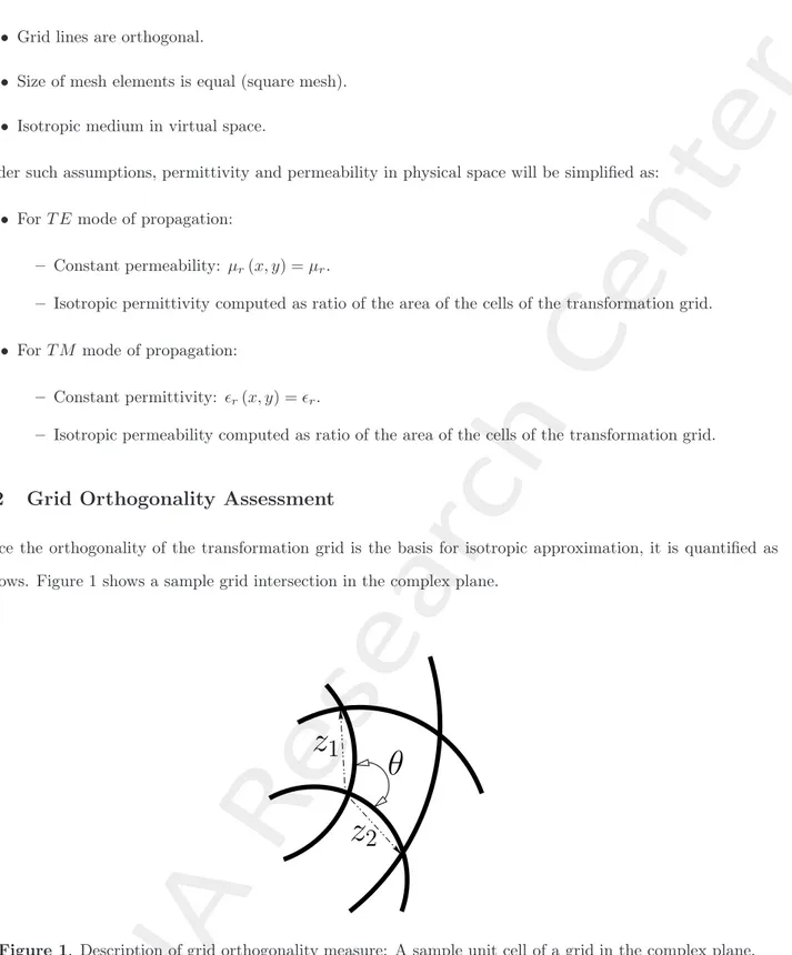
Since the orthogonality of the transformation grid is the basis for isotropic approximation, it is quantified as follows. Figure 1 shows a sample grid intersection in the complex plane.
θ
z
1
z
2
Figure 1. Description of grid orthogonality measure: A sample unit cell of a grid in the complex plane.
Referring to Figure 1, and using Euler’s notation, z1 = |z1| ej[arg(z1)], z2 = |z2| ej[arg(z2)], the internal angle θ
can be computed as
θ= arg (z1) − arg (z2) = arg
! z1
z2
" . The offset from orthogonality χ can then be evaluated as
3
Numerical Results
3.1
Edge to Circular Transformation
Goal: Reshaping of conformal array
Test Case Description
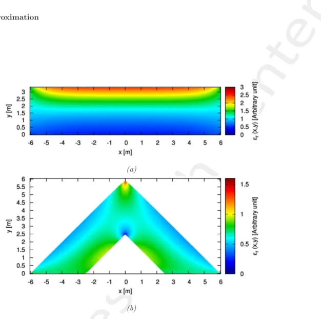
A 2D problem is considered and the transformation is described pictorially in Figure 2. Figure 2(a) shows the virtual array, Figure 2(b) the rectangular intermediate medium while Figure 2(c) shows the setup of the actual physical array. The main purpose of this test case is to investigate the ability to synthesize metamaterial lenses capable of transforming a conformal arrays(specifically in the form of a wedge in 2D) into a standard circular array. The synthesized array is expected to have uniform beam shape when being steered.
In Figure 2, the dimensions a, w, γ and the inter element spacing in the virtual space (d!!) are parameters taken
from design specification (free parameters) and all other dimensions depend on these parameters (a, w, γ and
d
!!
x
!!
a
!!
y
!!
h
!!l
!!
w
!!
( a)t
!
l
!
h
!x
!
w
!
y
!
(b)γ
w
a
l
h
y
x
(c)Simulation Parameters
• Array of Isotropic radiators.
• Number of Array Elements: N = 20. • Frequency of operation: ν = 600M Hz • Wavelength in free space: λ = 0.5m Physical Object Parameters:
• Width of transformation region: w = 5λ. • Length of the edge: a = 5λ.
• Angle of the edge: γ = 900.
Virtual Object Parameters:
• Array of point sources uniformly distributed along a circular contour, symmetric with respect to y!!axis.
• Radius of the contour of the array: a!!= a = 5λ.
• Width of transformation region: w!!= w
sinγ
2 = 5.876λ.
• Element Spacing along the circular contour: d!!= λ
2.
• Uniform Amplitude Excitation: I!
n= 1.
• Pattern steered to φ!!
s = 600with phase excitation defined as[6]:
ϕ! n= −2π λ a !× cos (φ!! s− φ!!n) . (30)
where φn is the angular position of the nth radiating element.
Transformation Parameters:
• Number of grid lines along x!− axis: xgrid = 251.
Full wave simulation Parameters:
• Two dimensional problem. • T E waves.
RESULTS
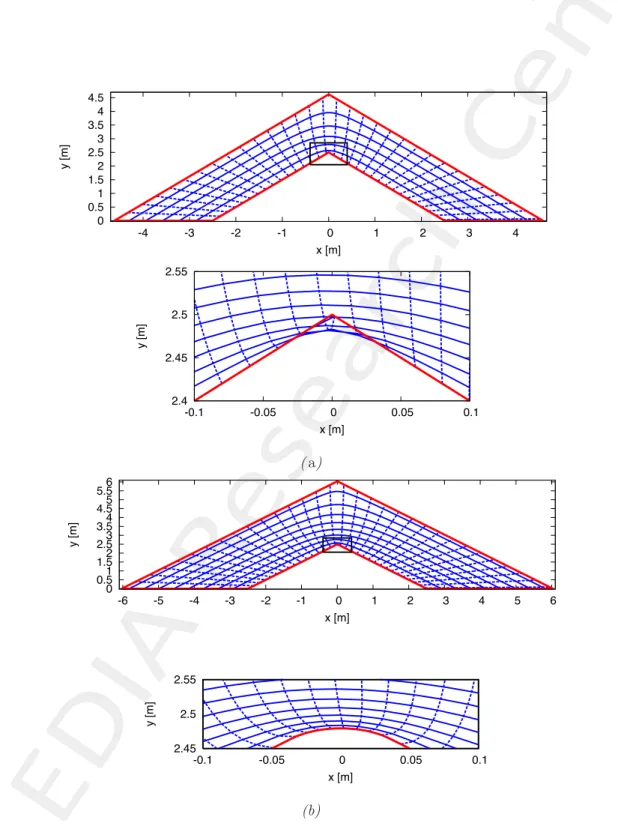
There was problem in the transformation. Due to the sharp corner going into the transformation region, part of the grid was distorted (Figure 3(a)). It is difficult (perhaps impossible) to interprete the distorted grid in terms of 2D material property distribution. To solve this problem, a fillet was applied at the internal corner and the distortion was avoided. The radius of the fillet applied is 2% of the edge length (0.02 × a = 0.1λ).
0 0.5 1 1.5 2 2.5 3 3.5 4 4.5 -4 -3 -2 -1 0 1 2 3 4 y [m] x [m] 2.4 2.45 2.5 2.55 -0.1 -0.05 0 0.05 0.1 y [m] x [m] ( a) 0 0.5 1 1.5 2 2.5 3 3.5 4 4.5 5 5.5 6 -6 -5 -4 -3 -2 -1 0 1 2 3 4 5 6 y [m] x [m] 2.45 2.5 2.55 -0.1 -0.05 0 0.05 0.1 y [m] x [m] (b)
Figure 3. Detail of the internal corner of the physical medium: a) sharp corner and (b) with fillet applied to the corner.
RESULTS
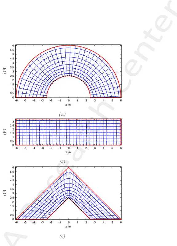
Transformation Grid 0 0.5 1 1.5 2 2.5 3 3.5 4 4.5 5 5.5 6 -6 -5 -4 -3 -2 -1 0 1 2 3 4 5 6 y [m] x [m] ( a) 0 0.5 1 1.5 2 2.5 3 -6 -5 -4 -3 -2 -1 0 1 2 3 4 5 6 y [m] x [m] (b) 0 0.5 1 1.5 2 2.5 3 3.5 4 4.5 5 5.5 6 -6 -5 -4 -3 -2 -1 0 1 2 3 4 5 6 y [m] x [m] (c)Figure 4. Transformation Grids: (a) Virtual space, (b) Intermediate space and (c) Physical space. The radiating elements are shown by the black dots.
Observations:
• The medium is discretized into: 250 × 68.
RESULTS
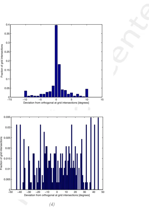
Grid orthogonality assessment.
(a)
−150 −10 −5 0 5 10 15 0.05 0.1 0.15 0.2 0.25 0.3 0.35 0.4
Fraction of grid intersections
Deviation from orthogonal at grid intersections [degrees]
(c) −500 −40 −30 −20 −10 0 10 20 30 40 50 0.005 0.01 0.015 0.02 0.025 0.03 0.035
Fraction of grid intersections
Deviation from orthogonal at grid intersections [degrees]
(d)
Figure 5. Transformation grid orthogonality test: (a),(c) primary transformation, (b),(d) secondary
transformation.
Observations:
• The first transformation is nearly orthogonal, Figure 5(a) and Figure 5(c).
• Large offset from orthogonality is observed for the secondary transformation because of the straight line edges and sharp corners, Figure 5(b) and Figure 5(d).
RESULTS
Exact values of permittivity.
!!!
vz = !!vz = !vz= !!!zv= !!zv= !zv = µ!!vz = µ!vz= µvz= µ!!zv= µ!zv = µzv = 0 where v ∈ {x, y}).
(a) (b)
(c) (d)
(f ) (g)
(h) (i)
(j)
Figure 6. Components of the permittivity tensor in the (a)-(e) intermediate medium, (f )-(j) physical medium.
Observations:
• Since the virtual medium is free space (!!!
r = µ!!r = 1), the permeability tensor in the intermediate and
physical medium, is the same as that of permittivity, i.e µ!= !!, µ = !.
• In the intermediate medium, the quantities µ!
xy = !!xy and µ!yx = !!yx are near zero whereas µ!xx= !!xxand
µ!
yy= !!yyare near unity except at the edges. As a result, pure Isotropic approximation can be made for
T E waves.
RESULTS
Isotropic approximation
(a)
(b)
Figure 7. Isotropic permittivity of the (a) intermediate (b) physical medium.
Observations:
• This approximation is valid under the assumption that the grids in virtual space are “nearly” orthogonal. Looking at Figure 5, this assumption is much better satisfied for the primary transformation.
• Permittivity value bounds:
– 0.4494 ≤ !!
r≤ 2.4728 in the intermediate space (Figure 7(a)).
RESULTS
Simulation Results
(a)
(b) (c)
(d) (e)
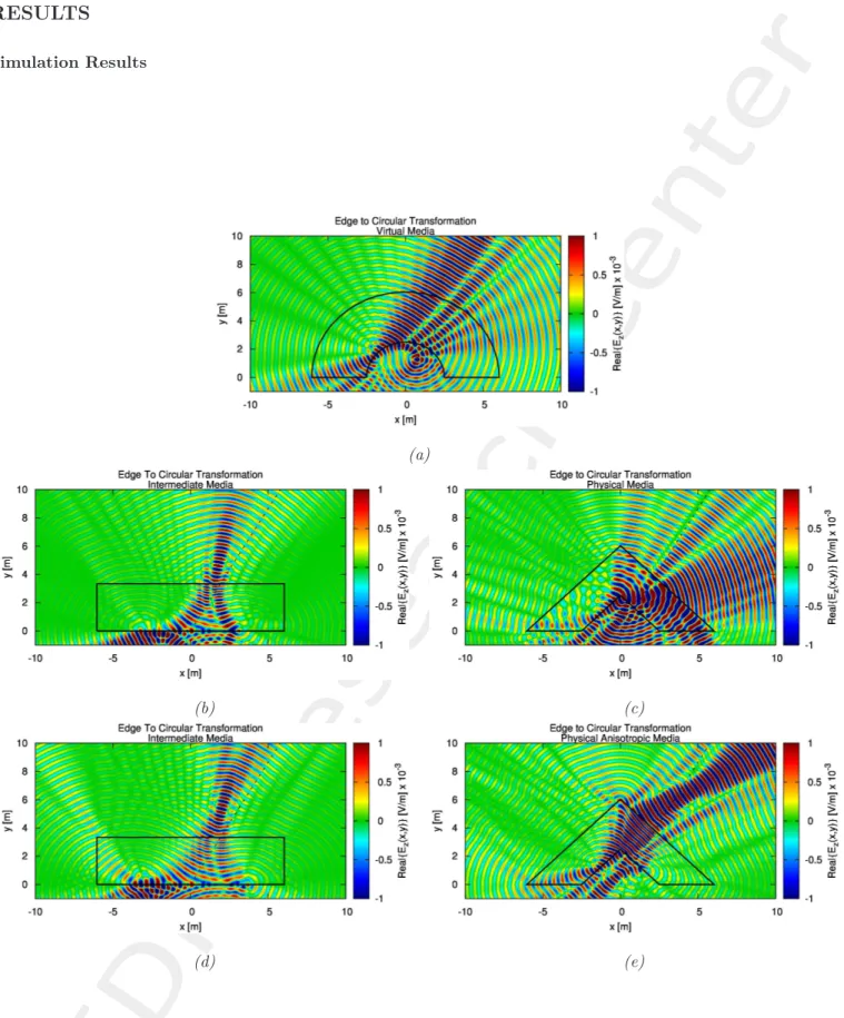
Figure 8. Normal component of the electric field: (a) Virtual space, (b) Intermediate space with Isotropic
approximation, (c) Physical space with Isotropic approximation, (d) Intermediate space with full Anisotropic
parameters and (e) Physical space with full Anisotropic parameters. The steering angle (φs= 600) is shown
Observations:
• There is no significant difference between the isotropic approximation and anisotropic implementations in the intermediate space (Figures 8(b) and (c). See also Figure 9). This validates the isotropic approxima-tion.
• The field distribution in intermediate and physical space is not steered to the desired angle. In addition the field does not resemble a directed/steered radiation.
RESULTS
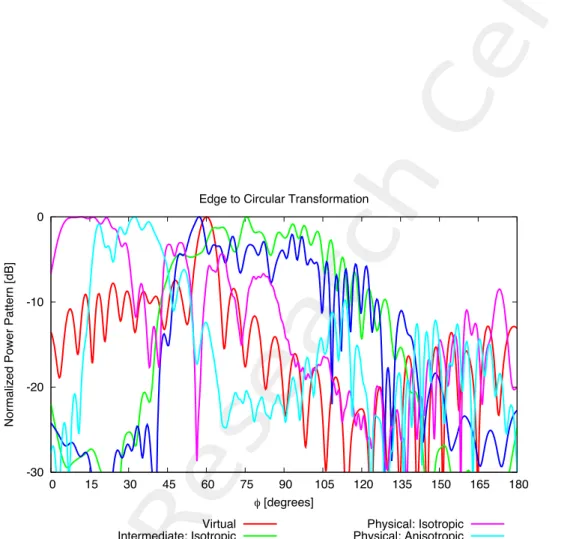
Comparison of power patterns
-30 -20 -10 0
0 15 30 45 60 75 90 105 120 135 150 165 180
Normalized Power Pattern [dB]
φ [degrees]
Edge to Circular Transformation
Virtual Intermediate: Isotropic Intermediate: Anisotropic
Physical: Isotropic Physical: Anisotropic
RESULTS
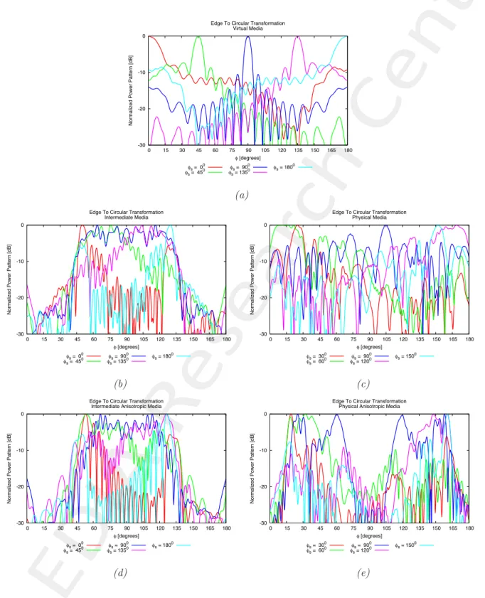
Comparison of power patterns
Several snapshots of the pattern at different steering angles is presented here.
-30 -20 -10 0
0 15 30 45 60 75 90 105 120 135 150 165 180
Normalized Power Pattern [dB]
φ [degrees] Edge To Circular Transformation
Virtual Media φs = 00 φs = 450 φs = 900 φs = 1350 φs = 1800 (a) -30 -20 -10 0 0 15 30 45 60 75 90 105 120 135 150 165 180
Normalized Power Pattern [dB]
φ [degrees] Edge To Circular Transformation
Intermediate Media φs = 00 φs = 450 φs = 900 φs = 1350 φs = 1800 -30 -20 -10 0 0 15 30 45 60 75 90 105 120 135 150 165 180
Normalized Power Pattern [dB]
φ [degrees] Edge To Circular Transformation
Physical Media φs = 300 φs = 600 φs = 900 φs = 1200 φs = 1500 (b) (c) -30 -20 -10 0 0 15 30 45 60 75 90 105 120 135 150 165 180
Normalized Power Pattern [dB]
φ [degrees] Edge To Circular Transformation
Intermediate Anisotropic Media
φs = 00 φs = 450 φs = 900 φs = 1350 φs = 1800 -30 -20 -10 0 0 15 30 45 60 75 90 105 120 135 150 165 180
Normalized Power Pattern [dB]
φ [degrees] Edge To Circular Transformation
Physical Anisotropic Media
φs = 300 φs = 600 φs = 900 φs = 1200 φs = 1500 (d) (e)
Figure 10. Plots of normalized power patterns at different steering angles: (a) Virtual array, (b) Intermediate Medium with Isotropic approximation, (c) Physical Medium with Isotropic approximation, (d) Intermediate
Comparison of power patterns: 3dB Beam Width
The 3dB beam width of the the patterns of Figure 9 and Figure 10 for a range of steering angles are reported here. 0 5 10 15 20 25 30 0 15 30 45 60 75 90 105 120 135 150 165 180
3dB Beam Width [degrees]
φs [degrees]
Circular to Linear Array Transformation
Virtual Intermediate: Isotropic Intermediate: Anisotropic
Physical: Isotropic Physical: Anisotropic
Figure 11. Comparison between normalized power patterns: Plot of beam width at different steering angles.
Observations:
• The beam width of the virtual circular array is uniform around the middle and varies at the ends. This is because the aperture of the array does not cover the circumference of a complete circle. The array
3.2
Edge to Circular Transformation: Matched Boundary
Goal: Reshaping of conformal array: solve the problem caused by refraction at metamate-rial boundary
Test Case Description
To investigate the refraction problem observed in the previous results (Figure 8), a modified transformation is presented here. Refraction will be avoided, if the metamaterial property (permittivity and permeability) is matched to the exterior region (air) at the interface. To realize such transformation, the transformation grids have to have the same shape at the interface. Towards this end, the following transformations (Figure 12) are proposed. The dimensions used in these transformations is the same as the previous test case listed in page 10. The only exception being the reduction in number of samples along x-axis to 201 (xgrid = 201) because the size of the metamaterial region is smaller in this case. For the same reason stated in page 11, a fillet is applied to the internal corner in the physical object; the radius of the fillet in this case is 5% of a(0.05 × a = 0.25λ).
d
!!
x
!!
a
!!
y
!!
h
!!l
!!
w
!!
( a)t
!
l
!
h
!x
!
w
!
y
!
(b)a
l
h
y
x
γ
w
(c)RESULTS
Transformation Grid 0 0.5 1 1.5 2 2.5 3 3.5 4 -4 -3 -2 -1 0 1 2 3 4 y [m] x [m] ( a) 0 0.5 1 1.5 2 -4 -3 -2 -1 0 1 2 3 4 y [m] x [m] (b) 0 0.5 1 1.5 2 2.5 3 3.5 4 -4 -3 -2 -1 0 1 2 3 4 y [m] x [m] (c)Observations:
• The medium is discretized into: 200 × 58.
• Approximate dimension of each cell in intermediate space: λ
12.5 ×
λ 12.5.
RESULTS
Grid orthogonality assessment.
−300 −20 −10 0 10 20 30 0.01 0.02 0.03 0.04 0.05 0.06 0.07 0.08
Fraction of grid intersections
Deviation from orthogonal at grid intersections [degrees]
(c) −30 −20 −10 0 10 20 30 0 0.01 0.02 0.03 0.04 0.05 0.06 0.07
Fraction of grid intersections
Deviation from orthogonal at grid intersections [degrees]
(d)
Figure 14. Transformation grid orthogonality test: (a),(c) primary transformation, (b),(d) secondary transformation.
Observations:
RESULTS
Exact values of permittivity.
!!!
vz = !!vz = !vz= !!!zv= !!zv= !zv = µ!!vz = µ!vz= µvz= µ!!zv= µ!zv = µzv = 0 where v ∈ {x, y}
(a) (b)
(c) (d)
(f ) (g)
(h) (i)
(j)
Figure 15. Components of the permittivity tensor in the (a)-(e) intermediate medium, (f )-(j) physical
medium.
Observations:
• µ! = !!, µ = !.
• In the physical space, material property is matched at almost all parts of the the boundary. That is,
at the interface of metamaterial and air the following conditions are satisfied: !xx = !yy = !zz = 1,
RESULTS
Isotropic approximation
(a)
(b)
Figure 16. Isotropic permittivity of the (a) intermediate (b) physical medium.
Observations:
• Permittivity value bounds:
– 0.3144 ≤ !!
r≤ 36.45 in the intermediate space (Figure 31(a)).
RESULTS
Simulation Results
(a)
(b) (c)
(d) (e)
Figure 17. Normal component of the electric field: (a) Virtual space, (b) Intermediate space with Isotropic
approximation, (c) Physical space with Isotropic approximation, (d) Intermediate space with full Anisotropic
parameters and (e) Physical space with full Anisotropic parameters. The steering angle (φs= 600) is shown
Observations:
• The virtual object is the same as the previous test case without matching. (Figure 8(a) and Figure 17(a) ).
• The field is directed/scanned as desired in intermediate space both for isotropic and anisotropic configu-ration. (Figures 17(b) and (c)).
• The field distribution in physical space with isotropic approximation is not properly scanned (Figure 17(d)).
• The field distribution in physical space with anisotropic distribution is scanned as desired (Figure 17(e)). • No significant amount of refraction observed at the boundaries.
RESULTS
Comparison of power patterns
-30 -20 -10 0
0 15 30 45 60 75 90 105 120 135 150 165 180
Normalized Power Pattern [dB]
φ [degrees]
Edge to Circular Transformation Matched Boundary Virtual Intermediate: Isotropic Intermediate: Anisotropic Physical: Isotropic Physical: Anisotropic
RESULTS
Comparison of power patterns
Several snapshots of the pattern at different steering angles is presented here.
-30 -20 -10 0
0 15 30 45 60 75 90 105 120 135 150 165 180
Normalized Power Pattern [dB]
φ [degrees] Edge To Circular Transformation Matched Boundary Virtual Media
φs = 00 φs = 450 φs = 900 φs = 1350 φs = 1800 (a) -30 -20 -10 0 0 15 30 45 60 75 90 105 120 135 150 165 180
Normalized Power Pattern [dB]
φ [degrees] Edge To Circular Transformation Matched Boundary Intermediate Media
φs = 00 φs = 450 φs = 900 φs = 1350 φs = 1800 -30 -20 -10 0 0 15 30 45 60 75 90 105 120 135 150 165 180
Normalized Power Pattern [dB]
φ [degrees] Edge To Circular Transformation Matched Boundary Physical Media
φs = 00 φs = 450 φs = 900 φs = 1350 φs = 1800 (b) (c) -30 -20 -10 0 0 15 30 45 60 75 90 105 120 135 150 165 180
Normalized Power Pattern [dB]
φ [degrees] Edge To Circular Transformation Matched Boundary Intermediate Anisotropic Media
φs = 00 φs = 450 φs = 900 φs = 1350 φs = 1800 -30 -20 -10 0 0 15 30 45 60 75 90 105 120 135 150 165 180
Normalized Power Pattern [dB]
φ [degrees] Edge To Circular Transformation Matched Boundary Physical Anisotropic Media
φs = 00 φs = 450 φs = 900 φs = 1350 φs = 1800 (d) (e)
Figure 19. Plots of normalized power patterns at different steering angles: (a) Virtual array, (b) Intermediate Medium with Isotropic approximation, (c) Physical Medium with Isotropic approximation, (d) Intermediate
Comparison of power patterns: 3dB Beam Width
The 3dB beam width of the the patterns of Figure 18 and Figure 19 for a range of steering angles are reported here. 0 5 10 15 20 25 30 0 15 30 45 60 75 90 105 120 135 150 165 180
3dB Beam Width [degrees]
φs [degrees]
Edge To Circular Transformation Matched Boundary Virtual Intermediate: Isotropic Intermediate: Anisotropic Physical: Isotropic Physical: Anisotropic
Figure 20. Comparison between normalized power patterns: Plot of beam width at different steering angles.
Observations:
• The curve of beam width of physical array with isotropic configuration closely follows the virtual array as desired.
Acknowledgment
This work has been developed within the EMERALD Project funded by Autonomous Province of Trento - Calls for proposal “Team 2011”.
References
[1] D.-H. Kwon, “Quasi-conformal transformation optics lenses for conformal arrays,” IEEE Antennas Wireless Propag. Lett., vol. 11, pp. 1125-1128, Sept. 2012.
[2] S. A. Cummer, N. Kundtz, and B.-I. Popa, “Electromagnetic surface and line sources under coordinate transformations,” Physical Review Letters A, 80 033820, pp. 033820 1-7, Sept. 2009.
[3] Y. Luo, J. Zhang, L. Ran, H. Chen, and J. A. Kong, “New concept conformal antennas utilizing metama-terial and transformation optics,” IEEE Antennas Wireless Propag. Lett., vol. 7, pp. 509-512, Jul. 2008.
[4] D. C. Ives and R. M. Zacharias, “Conformal mapping and orthogonal grid generation,” In
AIAA/SAE/ASME/ASEE 23rd Joint Propulsion Conference, San Diego, California, Paper number 87-2057, June 1989.
[5] W. Tang, C. Argyropoulos, E. Kallos, W. Song and Y. Hao, “Discrete coordinate transformation for de-signing all-dielectric flat antennas,” IEEE Trans. Antennas Propag., vol. 58, no. 12, pp. 3795-3804, Dec. 2010.
[6] C. A. Balanis, Antenna Theory: Analysis and Design (3rd Ed.). Wiley, 2005.
[7] P. Rocca, M. Benedetti, M. Donelli, D. Franceschini, and A. Massa, "Evolutionary optimization as applied to inverse problems," Inverse Problems - 25th Year Special Issue of Inverse Problems, Invited Topical Review, vol. 25, pp. 1-41, Dec. 2009.
[8] P. Rocca, G. Oliveri, and A. Massa, "Differential Evolution as applied to electromagnetics," IEEE Antennas and Propagation Magazine, vol. 53, no. 1, pp. 38-49, Feb. 2011.
[9] G. Oliveri and A. Massa, "GA-Enhanced ADS-based approach for array thinning," IET Microwaves, An-tennas & Propagation , vol. 5, no. 3, pp. 305-315, 2011.
[10] G. Oliveri, F. Caramanica, and A. Massa, "Hybrid ADS-based techniques for radio astronomy array design," IEEE Transactions on Antennas and Propagation - Special Issue on "Antennas for Next Generation Radio Telescopes," vol. 59, no. 6, pp. 1817-1827, Jun. 2011.
[11] L. Poli, P. Rocca, G. Oliveri, and A. Massa, "Harmonic beamforming in time-modulated linear arrays," IEEE Transactions on Antennas and Propagation, vol. 59, no. 7, pp. 2538-2545, Jul. 2011.
[12] L. Poli, P. Rocca, L. Manica, and A. Massa, "Handling sideband radiations in time-modulated arrays through particle swarm optimization," IEEE Transactions on Antennas and Propagation, vol. 58, no. 4, pp. 1408-1411, Apr. 2010.
[13] L. Poli, P. Rocca, L. Manica, and A. Massa, "Time modulated planar arrays - Analysis and optimization of the sideband radiations," IET Microwaves, Antennas & Propagation, vol. 4, no. 9, pp. 1165-1171, 2010. [14] L. Lizzi, F. Viani, R. Azaro, and A. Massa, "Optimization of a spline-shaped UWB antenna by PSO,"
IEEE Antennas and Wireless Propagation Letters, vol. 6, pp. 182-185, 2007.
[15] L. Lizzi, F. Viani, R. Azaro, and A. Massa, "A PSO-driven spline-based shaping approach for ultra-wideband (UWB) antenna synthesis," IEEE Transactions on Antennas and Propagation, vol. 56, no. 8, pp. 2613-2621, Aug. 2008.
[16] P. Rocca, L. Manica, and A. Massa, "An improved excitation matching method based on an ant colony optimization for suboptimal-free clustering in sum-difference compromise synthesis," IEEE Transactions on Antennas and Propagation, vol. 57, no. 8, pp. 2297-2306, Aug. 2009.
[17] P. Rocca, L. Manica, and A. Massa, "Ant colony based hybrid approach for optimal compromise sum-difference patterns synthesis," Microwave and Optical Technology Letters, vol. 52, no. 1, pp. 128-132, Jan. 2010.
[18] P. Rocca, L. Manica, F. Stringari, and A. Massa, "Ant colony optimization for tree-searching based synthesis of monopulse array antenna," Electronics Letters, vol. 44, no. 13, pp. 783-785, Jun. 19, 2008.
[19] G. Oliveri and L. Poli, "Optimal sub-arraying of compromise planar arrays through an innovative ACO-weighted procedure," Progress in Electromagnetic Research, vol. 109, pp. 27-299, 2010.
[20] G. Oliveri, "Improving the reliability of frequency domain simulators in the presence of homogeneous metamaterials - A preliminary numerical assessment," Progress In Electromagnetics Research, vol. 122, pp. 497-518, 2012.
[21] I. Martinez, A. H. Panaretos, D. Werner, G. Oliveri, and A. Massa "Ultra-thin reconfigurable electro-magnetic metasurface absorbers," 2013 European Conference on Antennas and Propagation (EUCAP), (Gothenburg, Sweden), 8-12 April 2013.
[22] G. Oliveri, P. Rocca, D. H. Werner, E. Bekele, M. Salucci, and A. Massa, "Design and synthesis of innovative metamaterial-enhanced arrays" 2013 IEEE Antennas and Propagation Society International Symposium, (Orlando, USA), July 7-13, 2013.
[23] E. Martini, G. M. Sardi, P. Rocca, G. Oliveri, A. Massa, and S. Maci "Optimization of metamaterial WAIM for planar arrays", 2013 USNC-URSI National Radio Science Meeting, (Orlando, USA), July 7-13, 2013.