Technical Report CoSBi 09/2006
Beta-binders with Static Compartments
Maria Luisa Guerriero Universit´a di Trento [email protected]
Corrado Priami
CoSBi and Universit´a di Trento [email protected]
Alessandro Romanel CoSBi and Universit´a di Trento
This is the preliminary version of a paper that will appear in LNCS 4545:247-261, c 2007 Springer-Verlag available at www.springerlink.com
Abstract
We investigate the modeling of biological systems with static com-partments through Beta-binders, a recently developed process lus. Biological entities are represented as bio-processes and the calcu-lus is extended with the notion of compartment. Entities can either be internal to compartments or reside on compartment borders. Move-ment in and out of compartMove-ments is requested by internal objects and mediated by border objects. The extended calculus is equipped with the notion of locality, and various kinds of relations between actions are defined. Moreover, we compare our proposal with similar for-malisms and we show how to use the proposed calculus for modeling and analyzing the cAMP-signaling pathway in OSNs.
1
Introduction
Compartments are present in all biological systems: a cell is a compartment, which in turn contains other compartments (the most important of which is the nucleus). Compartments are fundamental for the evolution of biological systems, because they provide a means for isolating their content from the external environment, still allowing some exchange of information, mainly through membrane proteins.
Several languages have been proposed to model biological compartments (Brane calculi [1], BioAmbients [2], Beta-binders [3, 4]). All of them have some differences in the considered notion of compartment and in the kinds of operations allowed (see Sect. 6 for a discussion). We focus here on Beta-binders, a process calculus with a two level syntax. The main objects are called bio-processes that are boxes with typed interfaces and whose behavior is driven by simplified π-calculus [5] like processes that they enclose.
In Beta-binders the nesting of boxes is not allowed, but typed interfaces ensures that a virtual form of nesting can be represented. Modeling complex hierarchies, however, is quite a difficult task that is simplified by our current proposal. We rely on a general interpretation of bio-processes as structured communicating objects and we propose an extension with the notion of static compartments, that permits an intuitive representation of hierarchical struc-tures, still forbidding the explicit nesting of boxes.
The structure of compartments and boxes allows us to consider spatial relations between events, e.g. the location where a protein-protein interac-tion occurs. Therefore, we enrich the calculus with some locality relainterac-tions, both on compartments and on boxes. We adopt the transition system-based technique used in [6, 7] to define a locality relation for the π-calculus.
Ex-amples of use of locality relations in modeling bio-chemical systems are in [8].
In the next section we briefly describe a slightly variant of Beta-binders. In Sect. 3 we introduce the notion of compartments and in Sect. 4 we present the labeled semantics of Beta-binders; in Sect. 5 some locality relations are defined. In Sect. 6 we compare our proposal with some existing works, while the application of our proposal to a model of the cAMP-signaling pathway in OSNs is shown in Sect. 7. Finally some concluding remarks are presented.
2
Beta-binders
Beta-binders [3, 4] is a bio-inspired process calculus developed for better ad-here to the structure and dynamics of biological systems. By introducing the concept of affinity, the calculus relaxes the key-lock model of interac-tion, commonly assumed in classical process calculi, and hence it permits to model more correctly domains and interactions between enzymes and small molecules based on their types and affinities. In Beta-binders, pi-processes are encapsulated into boxes with interaction capabilities, called also bio-processes. Like the π-calculus, Beta-binders is based on the notion of naming. Thus, we assume the existence of a countably infinite set N of names (ranged over by lower-case letters).
The processes wrapped into boxes, also called pi-processes, are given by the following context free grammar:
P ::= nil
|
π. P|
P|P|
! π.Pπ ::= x(y)
|
xhyi|
expose(x, Γ)|
hide(x)|
unhide(x) .The π-calculus syntax is enriched by the last three prefixes for π to ma-nipulate the interaction sites of the boxes. The object y of the input prefix x(y) as well as the x of the expose(x, Γ) prefix act as binding occurrences. Hence we can define free fn and bound bn names as usual. Bio-processes are defined as pi-processes prefixed by specialized binders that represent inter-action capabilities. An elementary beta binder has the form β(x : Γ) (active) or βh(x : Γ) (hidden) where the name x is the subject of the beta binder
and Γ represents the type of x. With bβ we denote either β or βh. A
well-formed beta binder (ranged over by B, B1, B′, · · · ) is a non-empty string
of elementary beta binders whose subjects and types are all distinct. The function sub(B) returns the set of all the beta binder subjects in B. More-over, B∗ denotes either a well-formed beta binder or the empty string. The
any algebraic structure for which it exists a decidable equality procedure. Hereafter, we also assume that substitution is not defined over the elements in a type. Note also that we do not have restriction in pi-processes and ! is guarded. This choice is done to adhere to the implementation of the language developed so far [9], but the general case works perfectly with the following development in this paper.
Bio-processes (ranged over by B, B1, B′, · · · ) are generated by the
fol-lowing context free grammar:
B ::= Nil
|
B[
P] |
B k B .The system is a parallel composition of bio-processes that can be either the deadlock bio-process Nil or the elementary bio-process B
[
P]
. The se-mantics of bio-processes is given in [3] in terms of a reduction relation (−→), which uses a structural congruence relation (≡). We postpone the formal def-initions of these relations to the next sections. For their standard defdef-initions, see [3].3
Compartments
The way in which a biological system is modeled here with Beta-binders is a composition of boxes, where each box represents a biological entity. Although the nesting of boxes is forbidden, the typing for sites and the operational semantics ensures that a virtual form of nesting can be represented [4]. This model might be too abstract, but it has been chosen to keep the formalism as simple as possible.
Consider for example the system
S = B
k
B′k
B′′ where: • B = β(s : ∆2)[
s(v) . R]
• B′ = β(x : ∆ 0)[
xhzi . hide(x) . P]
• B′′ = β(y : ∆ 1)[
y(v) . Q]
and where α(∆0,∆1) > T h ∧ α(∆j,∆2) < T h with j ∈ {0, 1}.1 The affinity
between the types exposed by the boxes could give us an a idea of how the
1The value T h represents a context dependent threshold over which two types are
boxes are grouped in compartments. In fact, we could imagine that the first and the second boxes are in the same compartment and that the third box is in another one. However, this kind of virtual nesting is ambiguous and for each defined system several different hierarchical structures can be deduced. In fact all the following three compartmentalization would be valid:
Moreover, consider the movement of objects across compartments. Since types encode compartments, moving an object from a compartment to an-other one means changing the types of the sites properly, using sequences of hide, unhide and expose operations. As the complexity of the model grows, the number of necessary actions makes this approach not practical and difficult to manage.
For these reasons we decided to introduce a finer and more explicit notion of compartments. Since we do not want to diverge from the original language, we decided to maintain the representation of systems as parallel composition of bio-processes, enriching statically them with labels acting as unique names which specify their location.
3.1
The Abstraction
Our goal is to provide a simple framework for modeling systems with static compartments and movements of components across compartments. A com-ponent is a structured object that can interact with other comcom-ponents through an affinity interaction model. Moreover, the movement of components be-tween compartments is mediated by other components lying on compartment borders. From a biological point of view this can be seen as a system where molecules and complexes can change compartment through interaction with transmembrane proteins. However, since compartmentalization and move-ment of components across compartmove-ments play a critical role in computa-tional systems, our approach can be applied in different contexts and at different levels of abstraction.
3.2
Static Compartment Hierarchy
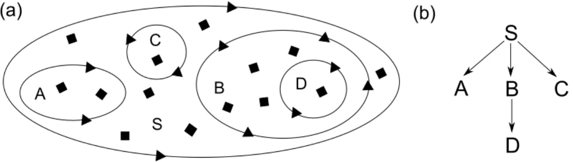
Consider the system represented in Fig. 1(a). There is an outside compart-ment (S) that represents the whole system. The system contains three sub-compartments (A, B, C). Moreover, the compartment B contains another compartment (D). The rectangles and the triangles are the components of
the system. In particular, rectangles represent components internal to com-partments, while triangles represent components that reside on compartment borders. We call i-components the internal components and b-components the border ones. We introduce the distinction between i- and b-components to be closer to real biological systems, in which objects residing on mem-branes and objects residing inside compartments have different and specific functions.
Figure 1: (a) System with static compartments; (b) The tree representation of the hierarchical structure of the compartments.
The static hierarchical structure of the system can be seen as a tree (Fig. 1(b)) where the nodes represent the compartments, and the numbers on the edges represent the numbering of the children.
Instead of using specific labels (e.g. S, A, ...) we can identify each compartment of the system with a sequences of natural numbers representing the position of the compartment inside the tree structure of the system, similarly to the Dewey’s indexes. Thus, the compartments of the system in Fig. 1 can be identified with the following sequences:
S → 0 A→ 0, 0 B → 0, 1 C → 0, 2 D→ 0, 1, 0 .
Since each component of the system is represented by a bio-process and resides in a particular compartment, we modify the syntax of Beta-binders by labeling bio-processes with the identifier of the compartment in which the bio-process resides. Moreover, to distinguish between components lying inside a compartment and components lying on compartment borders, we add to each bio-process a special marker representing the component type. Formally, the definition of bio-processes is modified as follows:
B ::= Nil
|
B[
P]
κs|
B k B κ ::= n|
κ, n .where n ∈ N specifies the position in the static structure and s ∈ {i, b} de-notes whether the component is an internal or a border one. As an example, a component lying on the border of the compartment D is represented with a bio-process B = B
[
P]
0,1,0b .3.3
Movements across Compartments
An i-component can move across a compartment border only through the interaction with a b-component residing on that border. This assumption mimics the role of transmembrane proteins in biological compartments. Since the calculus is based on a binary synchronous communication model, we still use affinity to mediate movement. Therefore, we modify the syntax of Beta-binders by adding the following new complementary actions prefixes:
π ::= · · ·
|
move(x)|
in(x)|
out(x)where x ∈ N . The move action synchronizes with in or out actions, thus giving to i-components the ability to move across compartment borders, and b-components the ability to control the flow direction. As an example, con-sider the system in Fig. 2(a), described in Beta-binders by the bio-process:
S = (B1 = B1
[
P1]
0i)
k
(B2 = B2[
P2]
0,0 b ) .Intuitively, B1 can move into the sub-compartment interacting through a
complementary move(x)/in(y) action with B2, where x and y are subjects of
binders with affine types. The new configuration of the system (Fig. 2(b)) after the movement of B1, is described in Beta-binders by the bio-process:
S′ = (B1′ = B1
[
P1′]
0,0 i )k
(B ′ 2 = B2[
P2′]
0,0 b ) .The detailed semantics is presented in the next section.
Figure 2: Example of movement across compartment.
4
Labeled Semantics
To introduce locality relations we first enrich the language and its semantics with labels that allow us to uniquely identify the location of bio-processes and compartments.
We define ϑ ∈ {k0,k1}∗and we use it to label bio-processes. We statically
replace each bio-process B
[
P]
κs with a labeled process ϑB[
P]
κs (where ϑ provides a linear encoding of the syntactical location of the sub-tree of B[
P]
κsin the syntax tree of the whole system). We chose this approach to take advantage of the syntax of the calculus and ease the implementation of the naming structure. We could have used any unique name generator just to distinguish the locations of bio-processes.
For instance, the bio-process βh(y : Σ)
[
P 0|
P1]
κ0 s0k
β(z : Σ)[
Q0|
Q1]
κ1 s1 is mapped to k0βh(y : Σ)[
P0|
P1]
κ0 s0k
k1β(z : Σ)[
Q0|
Q1]
κ1 s1.Each transition is labeled by a pair φ = hθ; κi, where κ is defined as in Sect. 3.2 and θ is defined by the following BNF-like grammar:
θ ::= ϑµ
|
ϑρ|
ϑhx(w), xhzii|
ϑhkjϑ0′x(w)8,k1−jϑ1′yhzi8i|
ϑhk0ϑ0joinP0,k1ϑ1joinP1i
|
ϑhkjϑ0ψ,k1−jϑ1move(x)iwhere µ ::= a
|
c|
d(with a ::= expose(x, Γ)|
hide(x)|
unhide(x), c ::= x(w)|
xhyi, and d ::=′x(w)8|
′xhyi8), ρ ::= splithP0, P1i
|
joinP and ψ ::= in(x)|
out(x).The first pair of labels is used to denote intra-communications (communica-tions within one bio-process), while the second one is used to denote inter-communications (inter-communications between different bio-processes); the third and the fourth ones are used to denote join and movement operations, re-spectively. Note that the definition of d allows us to distinguish between the input/output actions used in intra-communications (x(w) / xhyi) and the ones used in inter-communications (′x(w)8/ ′xhyi8). According to the
defini-tion of binders, y is a bound name in x(y), in ′x(y)8 and in expose(y, Γ).
We introduce two new sets of labels, with metavariable γ and δ respec-tively, that will be useful in the following:
γ ::= a
|
hc0, c1i δ ::= d|
ψ|
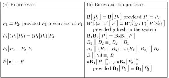
move(x) .Definition 1 The structural congruence over pi-processes, denoted by ≡, is the smallest relation which satisfies the laws in Table 1(a). The struc-tural congruence over bio-processes is identified by two relations, denoted respectively by ≡ and ≡c, that are the smallest ones which satisfy the laws in
Table 1(b).
Definition 2 The reduction relation −→ is the smallest relation over bio-processes defined by the axioms and rules in Table 2.
As in [3], fjoin and fsplit functions are user defined λ-calculus functions
which describe the aggregation and disaggregation of boxes and depend on the structure of bio-processes.
Table 1: Laws for structural congruence.
(a) Pi-processes (b) Boxes and bio-processes
B
[
P1]
≡ B[
P2]
provided P1 ≡ P2 P1≡ P2, provided P1 α-converse of P2 B∗β(x : Γ)ˆ[
P]
≡ B∗β(y : Γ)ˆ[
P {y/x}]
provided y fresh in the system P1
|
(P2|
P3) ≡ (P1|
P2)|
P3 B1B2[
P]
≡ B2B1[
P]
B1k
B2 ≡cB2k
B1 P1|
P2 ≡ P2|
P1 B1k
(B2k
B3) ≡c(B1k
B2)k
B3 Bk
Nil ≡cB P|
nil ≡ P ϑB1[
P1]
κ s ≡cϑB2[
P2]
κ s provided B1[
P1]
≡ B2[
P2]
5
Locality Relations
To define some locality relations on Beta-binders transitions we first need two auxiliary functions for each transition φ: act(φ) specifies the action executed, and comp(φ) specifies the compartment in which the action is executed.
act(hθ, κi) = θ comp(hθ, κi) = κ .
We first define some relations concerning compartments (i.e. the com-partments in which the actions triggering the transitions occur). Finally, we consider the level of bio-processes (i.e. the bio-processes involved in the transitions).
Based on the definition of localities described in [10], compartments are static localities: they do not change dynamically during execution, and hence they represent the sites in which events occur. Therefore, the relations in-troduced in the next section refer to the relative positions of the considered transitions. ϑ labels of bio-processes are, instead, dynamical localities: in fact they are built incrementally when actions are performed (actually, only split operations modify the labels by adding sublabels to the labels of the created bio-processes), and hence they represent, for each action, the ones that locally precede it.
Table 2: Axioms and rules for the reduction relation. (intra) P ≡ x(w) . P0
|
xhzi . P1|
P2 ϑB[
P]
κ s hϑhx(w),xhzii;κi −→ ϑB[
P0{z/w}|
P1|
P2]
κ s(inter) P ≡ x(w) . P1
|
P2 Q ≡ yhzi . Q1|
Q2 , where Xhϑhkjϑ0 ′x(w)8,k 1−jϑ1′yhzi8i;κli −→ Y X = ϑkjϑ0β(x : Γ) B∗0[
P]
κ0 s0k
ϑk1−jϑ1β(y : Σ) B ∗ 1[
Q]
κ1 s1, Y = ϑkjϑ0β(x : Γ) B∗0[
P1{z/w}|
P2]
κ0 s0k
ϑk1−jϑ1β(y : Σ) B ∗ 1[
Q1|
Q2]
κ1 s1provided α(Γ, Σ) ≥ T h and (κl= κ1−l∨ (κl= κ1−l, n ∧ sl= b ∧ s1−l= i))
(expose)
P ≡ expose(x, Γ) . P1
|
P2, y fresh in the system ϑB
[
P]
κ s hϑ expose(x, Γ);κi −→ ϑB β(y : Γ)[
P1{y/x}|
P2]
κ s (hide) P ≡ hide(x) . P1|
P2 ϑB∗β(x : Γ)[
P]
κ s hϑ hide(x);κi −→ ϑB∗βh(x : Γ)[
P 1|
P2]
κ s (unhide) P ≡ unhide(x) . P1|
P2 ϑB∗βh(x : Γ)[
P]
κ s hϑ unhide(x);κi −→ ϑB∗β(x : Γ)[
P1|
P2]
κ s (join) ϑϑ0B0[
P0]
κ sk
ϑϑ1B1[
P1]
κ s hθ;κi −→ ϑϑ0B[
P0σ0|
P1σ1]
κ sk
ϑϑ1Nilwhere θ = ϑ hϑ0join P0, ϑ1join P1i, ϑ0= k0ϑ′0, ϑ1= k1ϑ′1
provided fjoin(B0, B1, P0, P1) = (B, σ0, σ1) (split) ϑB
[
P0|
P1]
κ s hϑ splithP0,P1i;κi −→ ϑk0B0[
P0σ0]
κ sk
ϑk1B1[
P1σ1]
κ s provided fsplit(B, P0, P1) = (B0, B1, σ0, σ1)(in) P ≡ in(x) . P1
|
P2 Q ≡ move(x) . Q1|
Q2, provided α(Γ, Σ) ≥ T h and where Xhϑhkjϑ0in(x),k1−j−→ϑ1move(x)i;κ,niY X = ϑkjϑ0β(x : Γ) B∗0[
P]
κ,n bk
ϑk1−jϑ1β(y : Σ) B ∗ 1[
Q]
κ i, Y = ϑkjϑ0β(x : Γ) B∗0[
P1|
P2]
κ,n bk
ϑk1−jϑ1β(y : Σ) B ∗ 1[
Q1|
Q2]
κ,n i(out) P ≡ out(x) . P1
|
P2 Q ≡ move(x) . Q1|
Q2, provided α(Γ, Σ) ≥ T h and where Xhϑhkjϑ0out(x),k−→1−jϑ1move(x)i;κ,niY X = ϑkjϑ0β(x : Γ) B∗0[
P]
κ,n bk
ϑk1−jϑ1β(y : Σ) B ∗ 1[
Q]
κ,n i , Y = ϑkjϑ0β(x : Γ) B∗0[
P1|
P2]
κ,n bk
ϑk1−jϑ1β(y : Σ) B ∗ 1[
Q1|
Q2]
κ i (redex) B−→ Bφ ′ Bk
B′′−→ Bφ ′k
B′′ (struct) B1≡cB ′ 1 B1′ φ −→ B2 B1 φ −→ B25.1
Compartments Locality Relations
In this section a bunch of significant locality relations between transitions is defined, assuming a computation B0
φ0
−→ B1 φ1
−→ · · · φn
−→ Bn+1, according to
the relative position of the compartments in which the transitions occur. We end this section by discussing how our relations can be useful in biological systems.
Definition 3 (Same-compartment relation) We say that φnhas a
same-compartment dependency on φh (denoted with φh ≍ φn) if h < n and
comp(φh) = comp(φn).
With this relation we underline the fact that the two actions φh and φn
occur in the same compartment.
Definition 4 (Son-father relation) We say that φn has a son-father
de-pendency on φh (denoted with φh f φn) if h < n and (comp(φn), m) =
comp(φh) (m ∈ N).
This means that the compartment in which the action φh occurs is the
son of the compartment in which the action φn occurs.
Definition 5 (Father-son relation) We say that φn has a father-son
de-pendency on φh (denoted with φh g φn) if h < n and (comp(φh), m) =
comp(φn) (m ∈ N).
In this case, the compartment in which the action φh occurs is the father
of the compartment in which the action φn occurs.
Son-father and father-son relations can be easily generalized to sub-com-partment and super-comsub-com-partment relations respectively, by considering their transitive closures.
Definition 6 (Sub-compartment and super-compartment relations) Let ⊼ , (f)∗ be the transitive closure of f. We say that φn has a
sub-compartment dependency on φh if φh⊼ φn.
Let ⊻ , (g)∗ be the transitive closure of f. We say that φn has a
super-compartment dependency on φh if φh⊻ φn.
The relation ⊼ means that the compartment in which the action φh occurs
is a sub-compartment of the compartment in which the action φn occurs,
and ⊻ means that the compartment in which the action φn occurs is a
Note that φh ⊼ φn ⇒ h < n and (comp(φn), κ) = comp(φh), and that
φh⊻ φn ⇒ h < n and (comp(φh), κ) = comp(φn).
In the area of dynamical modeling of biological systems, locality relations can be useful for analyzing the spatial distribution of entities. For example, when observing transitions originated by an interesting event, we could be interested in investigating what happened in the same compartment before. The relation ≍ can be used for that. Similarly, we could use the other relations to study what happened in super- or sub-compartments.
5.2
Inter-boxes Locality Relation
In this section we define the inter-boxes locality relation between pairs of transitions in a computation: an inter-boxes locality relation exists between an activity A and an activity B if A and B are executed by pi-processes in the same bio-process. Our labels can be used as unique names for the transitions as they are linearizations encoding the position of the prefixes and processes originating the transitions in the syntax tree.
Definition 7 (Direct inter-boxes locality relation) Given a computa-tion B0
φ0
−→ B1 φ1
−→ · · · φn
−→ Bn+1, we say that φn has a direct inter-boxes
locality dependency on φh if h < n and act(φh) ⋖ act(φn) can be derived by
repeated applications of the following rules, where j ∈ {0, 1}. 1. kjθ ⋖kjθ′ if θ ⋖ θ′
2. γ ⋖ γ′
3. hkjϑ0δ0,k1−jϑ1δ1i ⋖ hklϑ′0δ′0,k1−lϑ′1δ1′i
if ((kjϑ0 = klϑ′0∧ k1−jϑ1 = k1−lϑ′1) ∨ (kjϑ0 = k1−lϑ′1∧ k1−jϑ1 = klϑ′0)) .
The rules listed above are applied recursively to a pair of actions θh, θn in
order to verify if there is an inter-boxes locality dependency between them. Since inter-boxes locality only concerns the bio-processes (and not their in-ternal structure), the recursive step is implemented by removing the common prefixes of θh and θn through rule 1, as long as they are relative to the
la-bels of bio-processes (k0 and k1). Then, at the end of the recursive steps
(i.e. if θh and θn refer to the same bio-process), either rule 2 or rule 3 could
be applied. Rule 2 states that actions on beta binders (i.e. expose, hide and unhide) and communications have an inter-boxes locality dependence on other actions on beta binders and other communications executed by pi-processes in the same bio-process. Rule 3 states that inter-communications
and transport operations have an inter-boxes locality dependence on other inter-communications and other transport operations if both operations are between the same bio-processes (i.e. each partner of one operation is executed by the same bio-process of one of the partners of the other operation).
Note that our mechanism is not affected by the associativity and com-mutativity of k, because the ϑ labels are attached statically to processes and updated in the operational semantics by the rules that affect the structure of the system.
The definition of the inter-boxes locality relation between two transitions of a computation is obtained by taking into account the transitive closure of the direct inter-boxes locality relation.
Definition 8 (Inter-boxes locality relation) Let < , (⋖)∗ be the tran-sitive closure of ⋖. Then, given a computation B0
φ0
−→ B1 φ1
−→ · · · φn
−→ Bn+1,
we say that φn has an inter-boxes locality dependency on φh if act(φh) <
act(φn).
From a biological point of view, when observing an interesting action performed by a bio-process, we could be interested in investigating other actions performed before by the same bio-process. The relation < can be used for that. Inter-boxes relation, together with compartments locality relations, can be useful for analyzing the spatial distribution of the actions executed by a bio-process.
6
Related Works
Several languages have been proposed to model biological compartments; the most common ones are Brane calculi [1] and BioAmbients calculus [2].
Differently from these calculi, the main aim of our work is to represent static compartments and movements of objects across them; hence, we just give an informal comparison on the usability of the languages with respect to different biological domains.
6.1
Brane Calculi
The main feature of Brane Calculi is that membranes are considered active elements and hence the whole computation happens on membranes: they can move, merge, split, enter in and exit from other membranes. A system is represented as a set of nested membranes, and a membrane as a set of actions; actions carry out the mentioned membrane transformations. The
main events that can be directly modeled are phagocytosis (the engulfment of a membrane by another one) and exocytosis (the expulsion of a membrane by another one). Moreover, operations such as mitosis (the splitting of one membrane in two membranes) and mating (the merging of two membranes) can also be described. On-membrane and cross-membrane communications can also be modeled.
Being Brane Calculi primarily concerned on membrane interaction, it per-mits to easily model membrane operations; on the other hand, it does not take the internal structure of membrane-bound compartments into account, therefore it is not easy to describe events such as protein activation, phos-phorylation, etc. Beta-binders, instead, is primarily focused on interaction between internal processes, hence compartments are used to describe the relative positions of the interacting bio-processes and to forbid interactions between processes which are in different compartments; hence, compartments (i.e. compartmental membranes) are static containers (it is not possible to create, destroy, or merge them) and bio-processes (i.e. proteins) can move across their borders. Therefore, operations involving membrane fusion, such as phagocytosis, exocytosis, mitosis and mating, cannot be modeled in Beta-binders by operations on compartments. For example, if compartments rep-resent cells, it is not possible to merge compartments to model cell mating; however, we point out that it is sufficient to change the level of abstraction, i.e. to represent cells with bio-processes and use fjoin and fsplit functions
to model such operations. Events that are not directly related to cellular membranes (e.g. phosphorylation) can easily be modeled by standard Beta-binders communications and operations on bio-processes interfaces.
Finally, in Brane Calculi everything is interpreted as a membrane, which means that membrane-bound cellular compartments (e.g. cells and organelles) and molecular compartments (e.g. proteins) are modeled in the same way: this seems a bit odd from a conceptual point of view. The proposed Beta-binders extension, instead, provides a double layer of compartmentalization (bio-processes and compartments), which permits a clear distinction between the two compartments types: when modeling cellular processes, cellular com-partments are represented by comcom-partments, while proteins are represented by bio-processes.
6.2
BioAmbients
BioAmbients calculus is an extension of the work described in [11], enriched with a concept of compartments similar to the one of Ambient calculus [12]. A system is represented as a set of nested ambients, and an ambient is a bounded compartment containing processes whose actions specify the
evo-lution of the system. Ambients can enter in and exit from other ambients (phagocytosis and exocytosis) and they can merge together (mating). π-calculus-style communications can occur within an ambient, between sibling ambients, and between father-child ambients.
Similarly to membranes in Brane calculi, ambients are used to represent both membrane-bound cellular compartments and molecular compartments (proteins and protein complexes). Moreover, BioAmbients does not provide an explicit way to model membrane proteins (they are implicitly considered by the primitives through which an ambient can allow another one to enter, exit or merge with). Hence, it is not easy to model complex interactions be-tween membrane proteins and internal proteins: the movement of an ambient in or out from another one is obtained by complementary actions executed by the two ambients. For example, there is no way to describe the expul-sion of a molecule (an ambient “m”) from a cell (an ambient “c” containing “m”), mediated by a membrane protein (an ambient “p” lying inside “c”). This, instead, can be easily done in Beta-binders. Finally, in BioAmbients it is not possible to move processes which are not lying in some ambient; hence, in order to describe the movement of small molecules across cellular membranes, they need to be enclosed within an ambient.
As previously stated, operations involving membrane fusion cannot be modeled in Beta-binders by operations on compartments (though they can be modeled by operations on bio-processes). In BioAmbients, instead, it is easy to model them (except mitosis, whose description in BioAmbients is not straightforward).
Entities in the same compartment can interact in BioAmbients though a local communication on a channel. In Beta-binders interaction is also done through inter-communications if the interfaces of the two entities are compatible.
Finally, it is not easy to model in BioAmbients events such as protein activations (in particular multi-step chains of proteins activations), which, instead, can be easily done in the proposed Beta-binders extension (as shown in the example described in the following section).
7
The cAMP-Signaling Pathway in OSNs
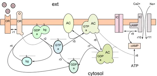
In this section we present how to use the extended Beta-binders formalism for modeling a biological system that includes membranes and membrane proteins. In particular, we model the cAMP-signaling pathway in olfactory sensory neurons (OSNs). The pathway describes how G protein-coupled receptors indirectly modulate the activity of ion channels via the action of
second messengers (Fig. 3).
Figure 3: The cAMP-signaling pathway in OSNs.
An odorant ligand O can bind with an odorant receptor OR through the reversible reaction r1, activating it. The active OR stimulates (r2) the G-protein GDPαβγ (denoted with GDPabg), causing the dissociation of the trimer in two active subunits GTPa and bg. At this point, GTPa can either hydrolyze (r3), returning GDPa, or activate the adenylyl cyclase (AC), his target protein (r5). If the reaction r3 takes place, the subunit GDPa reasso-ciates with the subunit bg (r4). If, instead, the reaction r5 takes place, the activation of AC produces, through the synthesis of ATP (r8), an increase in the concentration of the second messenger cAMP. A cAMP molecule can open, through a reversible binding (r9), the ion-channel IC, allowing Na+
and Ca2+molecules to enter. However, the hydrolysis of GTP to GDP causes
GTPa to dissociate from AC and reassociate with bg. For a more detailed description of the pathway we refer the reader to [13].
Table 3 shows the specification of the Beta-binders model of the presented pathway.2 Moreover, α(∆
k,∆j) > T h iff (k = j) ∨ (k = 4 ∧ j ∈ {5, 6}). The
parallel composition of all the defined bio-processes
S = BO
k
BORk
BGk
BACk
BATPk
BICk
BNa+k
BCa2+represents the initial configuration of the system, denoted with S. All the communications enabled by the bio-processes represent the reactions r1, · · · , r11 shown in Fig. 3, and all the intermediate configurations that the system S
2With kn
k we indicate the sequence kk· · · kk
| {z }
n
can reach through the execution of communications represent all the possible configurations of the biological system.
Table 3: Specification of the model.
O = xhzi . x(z) .O AC = y(z) .AC
OR = x(z) . unhide(y) . hide(y) . xhzi .OR cAMP = xhzi . x(z) .cAMP
A = yhzi .A IC = x(z) . unhide(y) . hide(y) . xhzi .IC GDP = x(z) .GTP M = in(y) .M
GTP = y(z) .GDP Na+= move(x) .Na+ Pα= yhzi .Pα Ca2+= move(x) .Ca2+
BO= k0β(x : ∆0)[O]0i BATP= k41k0β(x : ∆3) β(y : ∆2)[yhzi .cAMP]0,0i
BOR= k1k0β(x : ∆0) βh(y : ∆1)[OR|A]0,0b BIC= k51k0β(x : ∆3) βh(y : ∆4)[IC|M]0,0b
BG= k21k0β(x : ∆1)[GDP|Pα|Pβγ]b0,0 BNa+= k61k0β(x : ∆5)[Na+]0i
BAC= k31k0βh(y : ∆2)[AC]b0,0 BCa2+= k71β(x : ∆6)[Ca2+]0i
fsplitG(B, P0, P1) = fsplitAC(B, P0, P1) =
if(B[P0|P1] ≡ β(x : ∆1)[(GTP|Pα)|Pβγ]) if(B[P0|P1] ≡ βh(x : ∆1) β(y : ∆2)[(GDP|Pα)|AC]
then(βh(x : ∆
1), βh(x : ∆1), id, id) then(βh(x : ∆1), βh(y : ∆2), id, id)
else ⊥ else ⊥
fjoinG(B0, B1, P0, P1) = fjoinAC(B0, B1, P0, P1) =
if(B0[P0] ≡ βh(x : ∆1)[GDP|Pα]∧ if(B0[P0] ≡ βh(x : ∆1)[GTP|Pα]∧
B1[P1] ≡ βh(x : ∆1)[Pβγ]) B1[P1] ≡ βh(y : ∆2)[AC])
then(β(x : ∆1), id, id) then(βh(x : ∆1) β(y : ∆2), id, id)
else ⊥ else ⊥
Now consider one of the possible computations, in which, starting from the initial configuration S, the ion-channel IC is activated, causing the en-trance of a Ca2+ molecule:
φ1: hhk1k0′x(z)8, k0′xhzi8i; 0i φ6: hk21hk20′y(z)8, k1k0′yhzi8i; 0, 0i
φ2: hk1k0unhide(y); 0, 0i φ7: hk14hk0′xhzi8, k1k0′x(z)8i; 0, 0i
φ3: hk1hk0′yhzi8, k1k0′x(z)8i; 0, 0i φ8: hk51k0unhide(y); 0, 0i
φ4: hk21k0splithGTP | Pα, Pβγi; 0, 0i φ9: hk51hk0in(y), k21move(x)i; 0, 0i .
φ5: hk21hk20join GTP | Pα, k1k0join ACi; 0, 0i
By analyzing the computation with the locality relations previously de-fined, we can observe, for example, that φ4 has a father-son dependency on
φ1 (denoted with φ1g φ4), while φ6 has a same-compartment dependency on
φ9 (denoted with φ6 ≍ φ9).
From a biological point of view, these relations state that a spatial relation g and a spatial relation ≍ exist, respectively, between the dissociation of the G-protein GTPαβγ and the activation of the receptor OR, and between the entrance of a Ca2+ molecule and the activation of the target protein AC.
8
Conclusions and Further Work
We extend Beta-binders with compartments and localities. Since the nesting of boxes is forbidden, modeling hierarchies of compartments in the standard version of the calculus is not primitive. We overcome this limitation by intro-ducing the concept of static compartments. Compartments allow the repre-sentation of operations such as the movement of objects across compartment borders and the communication between internal and border objects.
Finally, some locality definitions have been introduced (both on compart-ments and on bio-processes/boxes) which can be useful when studying the spatial distributions of objects (and events) in complex systems.
Many further extensions are possible. One is to differentiate the var-ious types of border objects: transmembrane proteins and those lying on the internal/external side of the membrane. The definition of the calculus should be slightly modified in order to take those differences into account. In addition to this, most proteins cannot freely move on the membrane, hence interactions between proteins on the same membrane are not always possible: the position of the proteins is important. This could be considered by intro-ducing additional constraints, based on the position of bio-processes, which permits interactions solely between “near” (according to some definition of distance) bio-processes.
A simulator for the extended calculus is under implementation. This will allow us to test our framework on large scale biological problems.
References
[1] Cardelli, L.: Brane Calculi - Interactions of Biological Membranes. In: Proceedings of Workshop on Computational Methods in Systems Biology (CMSB’04). Volume 3082 of LNCS. (2005) 257–278
[2] Regev, A., Panina, E.M., Silverman, W., Cardelli, L., Shapiro, E.Y.: BioAmbients: an Abstraction for Biological Compartments. Theoretical Computer Science 325(1) (2004) 141–167
[3] Priami, C., Quaglia, P.: Beta binders for biological interactions. In: Proceedings of Workshop on Computational Methods in Systems Biology (CMSB’04). Volume 3082 of LNCS. (2005) 20–33
[4] Priami, C., Quaglia, P.: Operational patterns in Beta-binders. Transactions on Computational Systems Biology 1 (2005) 50–65
[5] Milner, R.: Communicating and Mobile Systems: the π-Calculus Cambridge University Press, 1999.
[6] Degano, P., Priami, C.: Non-interleaving semantics for mobile processes. Theoretical Computer Science 216(1–2) (1999) 237–270
[7] Degano, P., Gadducci, F., Priami, C.: Causality and Replication in Concurrent Processes. In: Proc. of Perspectives of System Informatics. Volume 2890 of LNCS. (2003) 307–318
[8] Curti, M., Degano, P., Priami, C., Baldari, C.T.: Modelling biochemical pathways through enhanced π-calculus. Theoretical Computer Science 325(1) (2004) 111–140
[9] Romanel, A., Dematt´e, L., Priami, C.: The BetaSIM System. Technical Report TR-03-2007, The Microsoft Research - University of Trento Centre for Computational and Systems Biology, 2007.
[11] Regev, A., Silverman, W., Shapiro, E.: Representation and simulation of biochemical processes using the π-calculus process algebra. In: Proceedings of Pacific Symposium on Biocomputing (PSB’01). Volume 6. (2001) 459–470 [12] Cardelli, L., Gordon, A.D.: Mobile Ambients. In: Proceedings of Conference on Foundations of Software Science
and Computation Structures (FoSSaCS’98). Volume 1378 of LNCS. (1998) 140–155
[13] Alberts, B., Johnson, A., Lewis, J., Raff, M., Roberts, K., Walter, P.: Molecular biology of the cell. Garland Science (2002)

![Table 2: Axioms and rules for the reduction relation. (intra) P ≡ x(w) . P 0 | xhzi . P 1 | P 2 ϑB [ P ] κ s hϑhx(w),xhzii;κi−→ ϑB [ P 0 {z/w} | P 1 | P 2 ] κs](https://thumb-eu.123doks.com/thumbv2/123dokorg/2954898.24667/10.892.161.728.237.1086/table-axioms-rules-reduction-relation-intra-hthhx-xhzii.webp)