A time deterministic communication stack for mesh networks

(1)

POLITECNICO DI MILANO

Master of Science in Computer Science and Engineering Dipartimento di Elettronica, Informazione e Bioingegneria

A time deterministic communication

stack for mesh networks

Relatore: William Fornaciari

Correlatore: Federico Terraneo

Tesi di Laurea di:

Federico Amedeo Izzo, 875328

(2)

(3)

List of Figures

5.1 Representation of TDMH superframe . . . 28

5.2 ISO/OSI model chart . . . 31

5.3 Comparison of two different stream periods . . . 32

9.1 Network topology from RTSS paper . . . 67

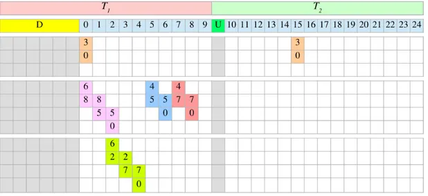
9.2 Schedule generated with the python simulator . . . 70

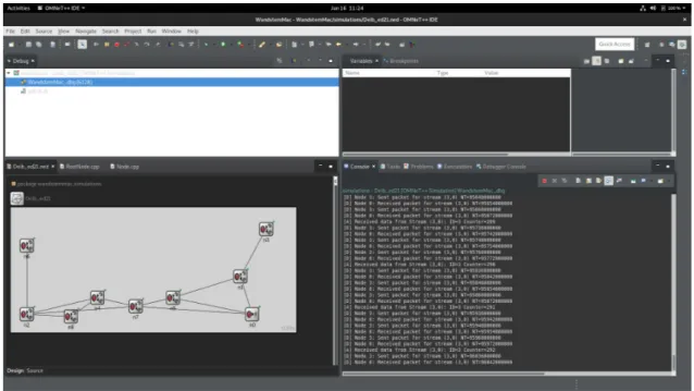
9.3 Debug view of the OMNeT++ simulator . . . 71

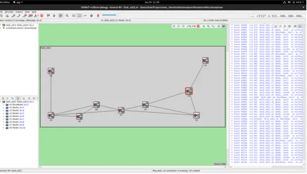
9.4 Simulation view of the OMNeT++ simulator . . . 72

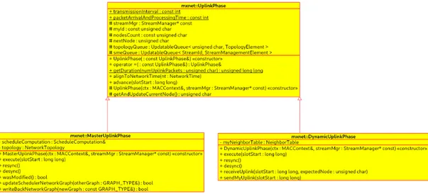
10.1 UML diagram showing polymorphism in the Uplink class . . . 74

10.2 Highlight of author’s contribution in TDMH codebase . . . 75

10.3 TDMH modules related to streams . . . 76

10.4 FSM model of master schedule distribution . . . 82

10.5 FSM model of master schedule application . . . 83

10.6 FSM model of dynamic schedule distribution . . . 84

10.7 FSM model of dynamic schedule application . . . 85

10.8 FSM model of streams in dynamic nodes . . . 89

10.9 FSM model of streams in master nodes . . . 90

10.10FSM model of servers in dynamic nodes . . . 91

10.11FSM model of servers in master nodes . . . 92

11.1 Diamond topology shown in OMNeT++ . . . 94

11.2 Diamond topology of the wired setup . . . 97

(8)

(9)

List of Tables

4.1 Comparison of TDMH with other IEEE 802.15.4 MACs . . . . 20

5.1 Possible choices for period with a tile duration of 100ms . 33 11.1 First experiment results with redundancy disabled . . . 96

11.2 First experiment results with triple redundancy . . . 97

11.3 Second experiment results with redundancy disabled . . . 101

11.4 Second experiment results with triple redundancy . . . 101

11.5 Third experiment results, reliability with single, double and triple spatial redundancy . . . 105

(10)

Chapter 1 Abstract

In these years communication between devices is becoming increasingly present in our lives. If we think about mobile phones or laptops, these de-vices couldn’t even fullfill their purpose without a working wireless connec-tion. Other fields where wireless networks are of paramount importance are for example the Internet of Things world and wireless data collection from sensors.

The most common wireless technologies can be divided roughly into high performance and low power technologies, two examples of high perfor-mance network technologies are WiFi and LTE while two low power network technologies are ZigBee or LoRa.

If we analyze the end-to-end latency of these technologies, we find that the latency of a WiFi network is around 1-5ms on a non congested network, but can quickly rise to 1s or more in presence of heavy traffic [1]. Meanwhile a ZigBee network have a normal latency of 50-350ms [2] which just like WiFi, can rise of several orders of magnitude in case of a congested network.

In this thesis we present TDMH, a wireless communication stack able to provide bounded latency, which means that the worst case network latency depends only on the network size and TDMH configuration and is independent from the network load.

(11)

The bounded latency makes TDMH suitable for real time applications like industrial control. TDMH is capable of managing multi-hop wireless mesh networks and its architecture allows to switch off the radio whenever a device doesn’t need to transmit or receive packets, this enables low power applications such as being employed on battery powered devices.

The author’s contribution to TDMH consists mainly in the scheduling and routing part of the network stack, which is the main focus of this thesis. The athor is responsible also for the design and implementation of several TDMH modules which are essential to the network stack operation.

You can find an overview of the main TDMH modules and the author’s contribution in sections 3.3 and 10.2.

(12)

Chapter 2 Sommario

In questi anni la comunicazione tra dispositivi è diventata sempre piú presente nelle nostre vite. Ad esempio i telefoni cellulari o i computer portatili perderebbero di funzionalitá se non ci fosse a disposizione una connessione wireless. Altri campi in cui le reti wireless sono fondamentali sono il mondo dell’Internet of Things e la raccolta dati da sensori wireless.

Le tecnologie wireless pi´u diffuse si possono categorizzare in reti ad alte prestazioni e reti low power, due esempi di tecnologie ad alte prestazioni sono il WiFi e LTE, mentre due tecnologie low power sono ZigBee e LoRa.

Se analizziamo la latenza di rete di queste tecnologie, troviamo dei valori intorno a 1-5ms per una rete WiFi non congestionata, ma questi valori pos-sono arrivare a 1s o pi´u in presenza di traffico elevato[1]. Mentre una rete ZigBee ha una latenza nominale di 50-350ms[2], che proprio come per il WiFi pu´o aumentare di diversi ordini di grandezza in una rete sotto carico.

In questa tesi viene presentato TDMH, uno stack di comunicazione wire-less in grado di fornire una latenza limitata, ovvero una latenza di rete nel caso peggiore che dipende solo dalla dimensione della rete e dalla configu-razione di TDMH e soprattutto `e indipendente dal carico di rete.

La latenza limitata rende TDMH adatto per applicazioni real time come il controllo industriale.

(13)

TDMH `e in grado di gestire reti wireless mesh con struttura multi-hop, inoltre TDMH permette di spegnere la radio quando un dispositivo non deve trasmettere o ricevere pacchetti, questo consente di risparmiare molta ener-gia, aprendo possibilit´a ad applicazioni low power, ad esempio su dispositivi alimentati a batteria.

Il contributo dell’autore a TDMH consiste principalmente nella parte di scheduling e routing dello stack di rete, questa tesi si concentrer´a princi-palmente su questi due aspetti. L’autore `e anche responsabile del design e dell’implementazione di alcuni moduli di TDMH che sono essenziali al fun-zionamento complessivo dello stack di rete.

Potete trovare una panoramica dei moduli principali di TDMH e del con-tributo dell’ autore a questi nelle sezioni 3.3 e 10.2.

(14)

Chapter 3 Introduction

3.1 An introduction to wireless networks

The importance of wireless networks in the world we live in is greatly increasing, since this technology can provide various advantages like mobility and flexibility.

Mobility is really important in many of the devices we use, for example mobile phones would be pretty useless without wireless technology, another advantage is that wireless technology doesn’t require a heavy infrastruc-ture and can be used in different environments, on the contrary in some of these environments running cables for a wired network may not be possible.

(15)

3.1.1 Case study: smart meters

An example of a low power wireless network that comes with a lightweight infrastructure is the wireless network used to remotely collect utility mea-surements from smart meters, like gas meters or water meters.[3]

In this kind of application as in many other wireless network applications, the low power consumption is fundamental.

For example if we decide to replace all the gas meters in a city with smart meters, we want these to have a battery life longer than two decades, to avoid facing too soon the great effort of replacing the batteries of all the meters in the city.

The technology used in smart utility meters is called LPWAN, which stands for Low Power Wide Area Network. The LPWAN technology is fairly recent, we will do an overview of other low power network technologies in chapter 4.

3.1.2 Case study: industrial control

Another successful application of wireless networks is industrial control. In this environment, a wireless network could be used to read sensor data coming from various parts of a plant, or even to send commands to actua-tors. Wireless technology in this application has significant advantages over a wired network counterpart, these advantages include lower costs, lower power consumption and higher flexibility. The flexibility could mean adding new sensor devices without changing the current infrastructure.

The network stack we present includes these advantages, and in addition introduces bounded latency, which reduces dramatically the uncertainty in data latency, enabling high precision readings and faster and more reliable actuations.

(16)

3.2 Goal of this work

Low power networks comes generally with one important disadvantage: the high latencies that derive from power saving techniques.

The goal of the work behind this thesis is to build a wireless network that while being low power, is capable also of achieving low latencies, in the order of nanoseconds. This low latency capability allows real-time applications.

The network stack presented is called TDMH, which stands for Time Deterministic Multi Hop, an acronym that recalls the deterministic nature of the stack given by the bounded latency, and its ability to handle

multi-hop networks.

3.3 Author’s contribution

The author’s contribution to the TDMH network stack consisted mainly in adding the missing scheduling and routing functionality to the stack, and additionally in designing, developing and testing several new modules of the network stack. The general goal of the work was to turn TDMH from being a Medium Access Control which included: time synchronization, network graph collection and packet sending, to a full fledged network stack, capable of opening and routing connections at runtime, and featuring several redundancy and data reliability options. This change is explained in detail in section 5.2.1.

(17)

Chapter 4 Literature review

4.1 Low power wireless protocols

As of note there is no wireless protocol that combines low latency with low power consumption, in fact high data rate protocols like WiFi

(IEEE 802.11) have a notoriously high power consumption [4], while low power protocols like ZigBee (IEEE 802.15.4) save power at the cost of in-creasing latency.

4.1.1 Low power listening

One of the techniques used to reduce the power consumption of wireless protocols is the one adopted in IEEE 802.15.4 networks called low power listening [5], this technique is able to reduce the radio reception power consumption at the expense of the transmission-side power consumption.

This technique consists in the sender transmitting a long preamble (100ms) before every packet (2ms) and the receiver checking periodically whether the channel is free or a carrier-wave is present (carrier sensing), in the latter case he can tell that a packet is incoming.

The check gives a statistical or deterministical certainty about receiving a packet, depending on the period at which the checks are performed.

(18)

This approach has its drawbacks, for example a collision problem when we have more than one node that wants to trasmit, these collisions have the effect of generating network delay. Another downside is the fact that transmitting a long preamble drains the battery of the transmitting nodes, also the receiving node may use more power than necessary if it senses the channel in the middle of the preable, because it has to receive the remaining half of the preamble (50ms) and the packet being sent (2ms). The biggest disadvantage of low power listening is the inefficient use of the radio channel, which is mostly occupied with preambles.

4.1.2 Channel access method

An important notion for understanding wireless protocols is the channel ac-cess method used. If we think of two wireless radios in range and operating on the same frequency, we know that only one of them can transmit at a given time and the other can only receive, because if two radios transmit at the same time on the same frequency, the information can get lost because of the interference between the two transmissions. This is the reason why we need a channel access method, to organize the transmissions of the different radios and reduce or eliminate the possibility of interference. The two most common channel access methods are CSMA/CA and TDMA [6].

CSMA/CA

CSMA/CA stands for Carrier Sense Multiple Access with Collision Avoid-ance and its principle is that a radio, before transmitting checks if the chan-nel is free, if that is the case the radio can transmit, if otherwise there is another transmission happening, the radio waits for a random time interval, called exponential backoff. This type of channel access is called a random channel access, its advantage is that it doesn’t require a centralized orches-tration of the transmissions, so it adapts easily to a changing environment, a

(19)

drawback of CSMA/CA is that with heavy traffic the latency can become very high, and in general is not predictable.

TDMA

TDMA stands for Time Division Multiple Access and is a channel access method that works by dividing the time in a given number of slots called timeslots, and making sure that for every timeslot at most one radio unit is transmitting. This technique allows to avoid collisions between transmis-sions of the same network, since the transmistransmis-sions are performed in different timeslots. The drawback of this technique is that it requires an orchestration of the transmissions, generally performed through a scheduling, we will see more of this technique because it is the one employed by TDMH. Among the advantages of TDMA, there is the bound latency, generally depending only on the propagation delay of the transmission and on the radio transmission and reception latency.

4.1.3 IEEE 802.15.4e

IEEE 802.15.4e [7] is an upgrade over existing standard IEEE 802.15.4, it introduces several new physical and MAC level standards, among which the most interesting ones are TSCH [8], DSME [9] and LLDN [10].

4.1.4 TSCH

It is the more developed standard, and the one most present in research. TSCH [8] is based on IEEE 802.15.4 peer-to-peer architecture, but em-ploys a TDMA-like architecture instead of CSMA/CA proposed by the IEEE 802.15.4 standard. A TSCH network uses beacons sent by the ”active” nodes of the network (IEEE 802.15.4 FFD, Fully Functioning Device) to synchronize the other nodes in the network. The ”active” nodes in the net-work build a schedule using a distributed algorithm, the schedule is used to

(20)

TDMA channel access mechanism.

Unfortunately, TSCH scheduling and schedule distribution are not de-fined in their RFC, in fact the design and development of these parts are left to the ones who implement the protocol. An example of TSCH implementa-tion is the 6TiSCH [11] protocol.

A possible limit of TSCH is that the protocol does not guarantee any boundaries on delays and real-time periods, the only guaranteed param-eter is the reliability of packet reception.

4.1.5 DSME

DSME [9] is a time-synchronized MAC protocol capable of multi-hop trans-missions, it provides some improvements over the IEEE 802.15.4 MAC speci-fication, like the multichannel capability. DSME employs a TDMA channel access mechanism like TSCH, and uses also channel diversity, which is the simultaneous use of different radio channels.

The DSME MAC transmits frames based on a time structure called multi-superframe, this structure contains 16 superframe slots, each of them is di-vided into a contention access period (CAP), and a contention free period (CFP), the CAP portion is contended between the nodes of the DSME net-work, while the CFP portion is scheduled and allocated to the single nodes.

The CAP section of the DSME frame is the more power hungry, since it requires a node to listen for the whole superframe to assess if the channel is free. For this reason DSME employs a scheme called CAP reduction, that gives priority to the scheduled and more power saving CFP mode.

TSCH frames are managed and scheduled like DSME’s CFP mode, and TSCH is able to get the power saving benefits of this mode.

(21)

4.1.6 LLDN

LLDN [10] is another MAC presented in the IEEE 802.15.4e standard. The LLDN MAC is limited to single hop topologies (star networks) and uses a single channel. It is aimed at data collection from sensors and is able to collect data every 10ms from 20 different sensors. The time structure of LLDN is composed by superframes and the nodes access the slots of the superframe by using CSMA/CA.

4.1.7 Comparison of TDMH with other protocols

See the table 4.1.

Protocol TDMH TSCH DSME LLDN

multi-hop yes yes yes no

guaranteed period yes no no yes topology type mesh cluster-tree cluster-tree star spatial redundancy yes no no no temporal redundancy yes feasible feasible feasible

channel spatial reuse yes yes (MODESA) no no management central. central./distr. central. central. Table 4.1: Comparison of TDMH with other IEEE 802.15.4 MACs

(22)

4.2 Scheduling

4.2.1 Introduction to scheduling

Scheduling is the operation of allocating of a set of resources to a number of agents requiring these resources. You can find a more in depth explaination of the problem in chapter 6. In the context of wireless sensor networks, and in particular of TDMA based networks, the resource available is a number of free timeslots, and the agents are the nodes of the network that want to send data through these timeslots.

Since the solution to this problem is not trivial, in TDMA based MACs we find a software module called scheduler that is able to solve this problem.

4.2.2 TSCH scheduling

The most similar scheduling algorithms found in literature are two algo-rithms proposed for the IEEE 802.15.4e TSCH MAC, called TASA [12] and MODESA [13].

4.2.3 TASA

TASA [12] stands for Traffic Aware Scheduling Algorithm, and is a proposed scheduling scheme for TSCH. It uses a centralized scheduling algorithm and requires that the master node has a complete topology information of the network.

The network topology information is composed of: • Logical network graph

• Physical connectivity graph

The TASA scheduling algorithm works as a combination of the matching and vertex coloring problems, which are solved by two algorithms. The two algorithms are applied in an iterative way, such that for every data slot the suitable links are selected step by step.

(23)

4.2.4 MODESA

MODESA [13] stands for Multichannel Optimized DElay time Slot Assign-ment, like TASA is a scheduling scheme proposed for TSCH. In MODESA, the nodes compete for a time slot if and only if they have something to trans-mit. Every node in a network scheduled with MODESA has a dynamic priority, which is calculated as remP ckt ∗ parentRcv, where remP ckt is equal to the number of packets present in the buffer, and parentRcv is the total number that the parent of the node has to receive.

The schedule is calculated by selecting for any timeslot the node that has the highest priority among all the nodes having data to transmit. A node can be scheduled in the current timeslot and channel only if it doesn’t interfere with nodes already scheduled on the same timeslot and channel, otherwise the node is scheduled on a different channel. This allows the spatial reuse of channels, since we can have multiple simultaneous transmissions on the same channel and timeslot, the check for interferences is performed on the connectivity graph, since the logical network graph does not use all the pos-sible physical links.

(24)

4.2.5 Compatibility with TDMH

The TASA and MODESA algorithms cannot be applied directly to the TDMH scheduling problem because of two core differences between TSCH and TDMH:

• TSCH employs channel hopping while TDMH uses a single channel

• TSCH uses a tree topology, while TDMH uses a mesh topology

The topology difference is the more important, since in a tree network all packets in the network are routed through the network coordinator, which is at the root of the network tree, this architecture simplifies a lot the scheduling problem, but reduces the overall network efficiency, since the distance between a node of the network and the network coordinator may be higher that the distance from the source node to the destination node in a mesh network.

Convergecast scheduling

There is another reason of incompatibility between TASA, MODESA and TDMH: TASA and MODESA are created for a convergecast network, while TDMH is not convergecast.

A convergecast network is a network where packets can only flow from a number of source nodes to a single sink node, that corresponds usually with the network coordinator [14].

This model is particularly suitable for to the usecase of collecting data from wireless sensors, without the need to send any data to the sensors itself.

TDMH is not a convergecast network, since it allows bidirectional com-munication between any pair of nodes of the network, so the scheduler should follow this requirement.

(25)

4.2.6 Considerations on spatial reuse of channel

The protocol we analyzed in this literature review have different approaches to spatial reuse of channel.

For example WirelessHART avoids on purpose the spatial reuse of channels when scheduling, this is done to avoid transmission failure due to interference between simultaneous transmissions [15].

On the contrary TSCH, in particular with the MODESA scheduler takes advantage of spatial reuse of channel by using a connectivity graph that is a superset of the network graph, containing all the link in radio range between nodes. Spatial reuse of channel is enabled for links without interference while links with interference are scheduled different channels [13].

(26)

Chapter 5 Project overview

5.1 Introduction to TDMH

TDMH is a real-time network stack capable of low power consumption. It is based on the IEEE 802.15.4 Radio standard and its network structure and algorithms are centralized. Regarding the network organization, TDMH is structured as a mesh network, and is capable of multi-hop transmissions.

TDMH relies heavily on time-synchronization, thanks to which all the nodes in the network have their internal clocks synchronized, this allows doing a TDMA (see section 4.1.2) access to the radio, without the need for carrier sensing, which we have seen in the literature review (chapter 4) having a great disadvantages in the form of latency and power consumption.

5.1.1 Time synchronization

The time synchronization part of TDMH is performed by employing the FLOPSYNC-2 [16] scheme, which is particularly effective in compensating the various sources of clock error and desynchronization, like jitter, temper-ature drift or clock errors caused by the PLL.

(27)

controller able to correct its non-idealities. This scheme is capable of high precision, below the µs, with a power consumption of less than 2.1µW . Other benefits of FLOPSYNC-2 include a monotonic and continuous clock, ex-cept for when the nodes resynchronize after losing connection to the network.

5.1.2 Master and Dynamic nodes

As hinted before, TDMH is a centralized protocol, which means that there is a special node in every network which orchestrates the entire network, this node is called the Master node and its tasks include keeping the main clock at which the other nodes of the network synchronize theirs to. The master node is also in charge of gathering the network topology and connection re-quests, and evaluate these two to grant or deny the opening of a Stream, this happens during the Scheduling phase, of which we will talk in the next chapters.

The other nodes of the TDMH network apart from the only Master node are called Dynamic nodes, this to indicate the fact that they might change their position in space, while the Master node is more likely to have a fixed position.

Dynamic nodes as opposed to the Master node, cooperate and forward each others’ transmission to perform three main tasks:

• Synchronizing their clock with the clock of the Master node

• Collecting the network topology graph

• Collecting information about connection requests or Streams

(28)

We have cited in this section the concept of Stream, which is specific to TDMH. A Stream is a connection between two arbitrary nodes of the network, and can be thought as the omologous of TCP/IP sockets.

TDMH Streams have some peculiarities with respect to Sockets, and we will talk in detail about these in the section 5.2.2 and following.

5.1.3 Protocol phases

As we said, TDMH is a TDMA protocol, and as such all the nodes have a notion of the network time, which is sychronized among the whole network. The network time is used to divide the time in different phases, which are used to carry out the various tasks of the network stack.

The phases are three, and can be distinguished based on the direction of information in of each of these.

The three network phases are:

• The Downlink phase in which the Master node distributes information to the rest of the network.

• The Uplink phase in which the Dynamic nodes gather information about the network and forward it to the Master node.

• The Data phase in which the Master and Dynamic nodes send appli-cation data to other nodes of the same network.

(29)

5.1.4 Tiled frame

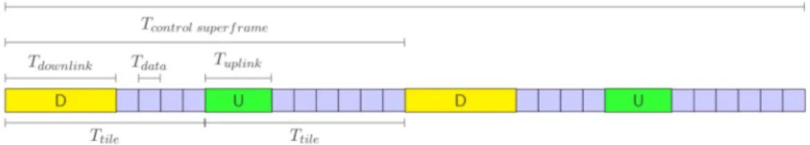
The network phases we listed are organized such that they can alternate and repeat in a sequence that is known to all the nodes of the network, as the exact number and sequence of the phases is part of the TDMH configuration.

In particular the time is divided into frames, which are time periods with a default lenght of 100ms, which are used to measure the time passed in the network stack.

The phases repetition is done by creating two types of frames called tiles, each of these tiles can be of two types, based on the TDMH phase is contains. The tiles alternate and repeat always in the same sequence, as we said before, this sequence if part of TDMH configuration. You can see an example of TDMH tiles in figure 5.1.

Figure 5.1: Representation of TDMH superframe

5.1.5 Downlink phase

The Downlink phase has two functions: its used to distribute information from the Master node to the other nodes in the network, but it is also used to keep the clocks of the Dynamic nodes synchronized with the one of the Master node. The part of the Downlink phase which is related to clock syn-chronization is called Timesync.

(30)

The information which is distributed consists in:

• Clock sychronization packets in the Timesync Downlink part

• Network schedule, in the Schedule Distribution part

• Signaling messages called Info Elements

Flooding

Packets in the Downlink phase are propagated in the network using a flooding technique, which takes advantage of the constructive interfer-ence. Constructive interference is the phenomenon that occurs when packets with the same content are transmitted at the same time by all the nodes of a certain hop distance, and the single resulting packet is received by all the nodes at the next hop. The technique used for flooding packets using con-structive interference is a modified version of Glossy [17].

5.1.6 Uplink phase

The Uplink phase is used to collect information from the Dynamic nodes towards the Master node, the information collected is the following:

• Network Topology which is used to synchronize the clocks

• Stream Management Elements which represent a request for open-ing a Stream.

5.1.7 Data phase

The Data phase is used by the Master and Dynamic nodes of the network to communicate and transfer application payloads over the network.

The Data phase works by performing the playback of a TDMA schedule that is computed by the Master node, and then distributed to the Dynamic nodes of the network in the Downlink phase.

(31)

5.2 Network stack design

The goal of the work behind this thesis was to expand and improve TDMH to make it able to be used to send data between two arbitrary nodes, without knowing a priori the details of the stream of data being sent in the network.

The main features of TDMH that were developed during this work are:

• Real-time streams to transmit data

with constant period and bounded latency

• Spatial and temporal redundancy of transmitted data for improved reliability and resilience

• An automatic scheduler for scheduling streams, taking count of the network topology and avoiding conflicts

• Spatial reuse of channels of the scheduled streams

• A schedule distribution system

The developement of these features needed a thorough design before the actual implementation, in this section we will present the design decisions behind the features of TDMH listed above.

(32)

5.2.1 From TDMH Mac to TDMH Stack

During the developement we realized that we were expanding the scope of TDMH from being a Medium Access Control to being a proper Network Stack.

This decision was not taken lightly, as we would have preferred to adhere to a layered network model like ISO/OSI [18]. However this was not possible for lack of support for crucial features of TDMH Streams in the layer 4 - Transport and upper. The unsupported features are periodic real-time streams and redundancy.

(33)

5.2.2 Streams and periods

The ability to send and receive data through real-time Streams is one of the core features of TDMH. The two main characteristics of TDMH Streams are constant period and bounded latency.

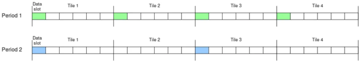
Period

The main feature of a real-time stream is its Period. The period determines what is the distance in time from one transmission of the stream and the following transmission of the same stream. You can see in figure 5.3 a comparison between a stream of Period 1 and another stream of Period 2.

Figure 5.3: Comparison of two different stream periods

Which period to choose depends largely on the needs of the application that will make use of the TDMH stream, in particular the choice must be based on the frequency at which the data needs to be sent or received. We know that the period can be calculated as the inverse of the frequency:

P = 1 f

For example a control loop running at a frequency of 1 Hz may specify a period of 1 s between one transmission and the next one, while an application reading data from a sensor at 10 Hz, needs to specify a period of 100 ms.

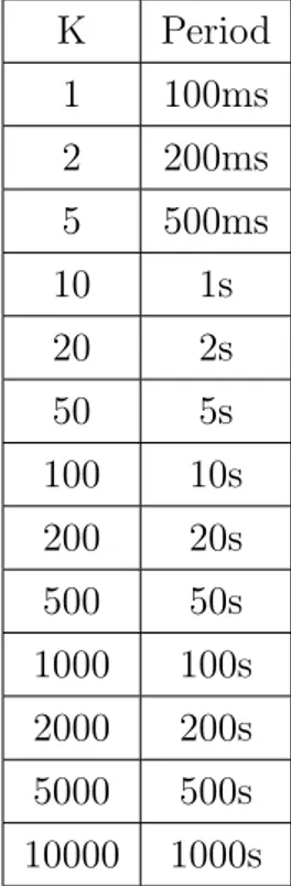
The period for a stream cannot be chosen in an arbitrary way, in fact there is a list of available periods, which are calculated in the following way:

(34)

K Period 1 100ms 2 200ms 5 500ms 10 1s 20 2s 50 5s 100 10s 200 20s 500 50s 1000 100s 2000 200s 5000 500s 10000 1000s

Table 5.1: Possible choices for period with a tile duration of 100ms

P (K) = K ∗ tile duration K ∈ N, K[1, N ]

Where tile duration is the time lenght of the TDMH tile (see chapter 5.1.4) and the K parameter indicates what multiple of tile duration we want to use as period.

With the tile duration default value of 100 ms, the possible periods are shown in table 5.1. Predefined period values will be denoted with P K, K ∈ [1, N ] for example P1 corresponds to 100ms, P50 to 5s and so on.

You may have noticed that only certain values of K are being shown on the table. In fact TDMH supports for K only integers with 1,2 or 5 as the leftmost figure, and a number of 0s for the other figures.

(35)

Length of a schedule

If we think of a schedule as a sequence of TDMA time slots, grouped in blocks of size equal to a TDMH tile. A schedule for a given stream must have some of the slots indicating the activity of the nodes of that stream, and is generally long a number of tiles equal to the K factor. If we denote the length of a schedule in number of tiles as schedule tiles we have that:

schedule tiles(P ) = K

When we have more than a stream, for example with two streams, the schedule length becomes the least common multiple of the periods of the two streams, this because the schedule needs to specify not only the slots used by a stream in its period, but all the possible combination of the slots used by the two streams, and the combinations of the slots are cyclic with a cycle long lcm(P 1, P 2). So for a number N of streams, the lenght of a schedule is:

schedule tiles(P 1, P 2, ..., P N ) = lcm(P 1, P 2, ..., P N )

The choice of numbers starting with either 1,2 or 5 comes from the Frobe-nius coin problem, in fact these three numbers can be used to obtain any higher number, and at the same time their lcm remains low [19].

Data rate

Choosing a period for a stream among the available ones means also deter-mining the data rate of the stream, since the corresponding data rate for a given period can be calculated in the following way

Data rate = payload size P eriod

(36)

5.2.3 Spatial and temporal redundancy

Reliability in receiving data over networks is fundamental, because

data loss can happen due to packet loss on wired network and interference or signal loss in wireless networks. Generally we want a way to mitigate the effect of data loss. In case of TCP/IP networks this is done by employing the TCP protocol itself, that makes sure that all data sent is also received, and if some data is lost along the way, it is retransmitted until it is received. TCP’s solution of error detection is not suitable to TDMH, because the packet loss effects are mitigated by resending data, and in a real-time network we don’t want to retransmit data based on the success of the previ-ous transmission, because doing that would create a non predictable increase of the latency. In fact in certain environments keeping the latency low is crucial, and a data that has been resent becomes old and possibly useless with respect to data delivered in time.

Our mitigation to the problem of data loss over radio interfaces comes in the form of transmission redundancy, in pratice data is sent two or three times within a period, to increase the probability of receiving at least one of the two or three copies of the data.

In particular TDMH supports two kind of redundancy:

• spatial redundancy: the two copies are sent over two different paths on the network (possibly without common intermediate nodes)

• temporal redundancy: the two copies are sent over the same path Clearly spatial redundancy is not always applicable in fact we may not have two paths without common intermediate nodes, in this case the scheduler will downgrade the redundancy type from spatial to temporal. Finally, it is important that the two paths do not have common interme-diate nodes, because these nodes would become the single point of failure

(37)

of the redundant stream.

5.2.4 Spatial reuse of channels

We wanted to apply another optimization to TDMH, since it is a TDMA network in which the master node knows and decides exactly in which instant every node of the network is going to send or receive messages on the radio. We decided to develop an interference model based on the network graph, to enable the spatial reuse of channels, that is the possibility for two or more nodes to send and receive packets simultaneously.

The simultaneous transmissions are allowed by the scheduler once it verifies that an interference cannot happen.

Summarizing, in a TDMA without spatial reuse, only one node in the network can transmit at a given time

Without spatial reuse of channels

1 2 3 4 5 6

T1 T2 T3 T2 T4 With spatial reuse of channels

1 2 3 4 5 6 T1 T3 T2

T2 T4

As previously said, the spatial reuse of channel is possible thanks to the interference check performed in the scheduler, which will be explained in the following section.

(38)

5.2.5 Interference check in scheduler

To model the radio interference between two nodes transmitting and re-ceiving at the same time, we start from the following assumptions:

• Two nodes in radio range are connected in the topology map

• Two nodes not connected in the topology map do not interfere with each other

The case in which two nodes are too distant to communicate properly but close enough to interfere each other is considered unlikely, because of the power capture and delay capture effects of the O-QPSK modulation employed [17].

Interference hypotesis

We have an interference if and only if we have one of these two situations: • A node is trasmitting and at least one of its neighbors is receiving

for a different transmission.

• A node is receiving and at least one of its neighbors is transmitting for a different transmission.

The four possible cases are summarized in this truth table: Node A Node B Interference

TX RX YES

TX TX NO

RX TX YES

(39)

Chapter 6 Scheduling: Theory

6.1 Problem statement

Scheduling in Computer Science generally means finding the best mapping between a set of jobs and the resources that can fullfill these jobs. This mapping is usually done by following a certain criterion, with the aim of maximizing a particular metric, for example fairness of use or quality of service. An example of scheduling is usually found in Operating Systems Architecture, in which the so called scheduler manages the allocation CPU time to Processes. In this case the metric can be from keeping the latency of a given process low to ensuring the fair use of the CPU among Tasks.

In the case of TDMH, being a TDMA network stack, the resources we are talking about are the slots of time, and the jobs to allocate are the trans-missions from the nodes of the network.

More in detail: When an application running on a TDMH enabled node wants to send data to another node in the same network, it requests the TDMH stack running on the node to open a Stream to that other node. We can think of a TDMH Stream as omologous to a TCP/IP socket.

(40)

This request gets forwarded by the network to the master node, the spe-cial node that coordinates the network, the master node can evaluate the stream request, and basing its decision on the current network topology, other opened streams and network configuration, decide if it is possible to open the requested stream and which TDMA time slots to allocate it to.

A Stream request is composed by the following information: • Source node ID

• Destination node ID

• Source Port

• Destination Port

• Period

• Size of the payload (in packets)

• Redundancy level

The Network Topology of TDMH is defined as a partial mesh, or a generic graph that is not fully connected, in which:

• Graph nodes represent the physical nodes forming the network

• Graph edges mean that the two nodes are in radio range

The Network Configuration of TDMH contains information about how the superframe is structured, which slots of the TDMA frame are available for data transmission and which other are needed for the other TDMH phases and cannot be used for data.

(41)

6.1.1 Routing and Scheduling

An important distinction to make is between the Routing and Scheduling problems, both of them are required to be solved in the scheduling of a generic Stream, but they are entirely different.

Scheduling

We previously said that the Scheduling problem consists in placing a re-quested stream in the suitable TDMA time slots.

This placement can be made by directly running the Scheduler algo-rithm only for Streams connecting two nodes in radio range, this situation can be seen in the topology as a graph edge connecting the two nodes in the Network graph.

The type of stream we just described is called single-hop, but they are not the only type of stream admitted by TDMH, in fact TDMH also supports multi-hop streams.

Routing

Multi-hop streams are data communication between two nodes that are not in direct radio range, but are still connected in the network graph, so the data can be sent by the source, forwarded by one or more intermediate nodes in the network and finally be received by its destination.

The Routing problem is the task of finding the best sequence of con-nected intermediate nodes between source of destination to route the multi-hop stream through the network.

The TDMH Router accepts as input a single multi-hop stream, and pro-duces as output a path on the graph, then converted to a list of two or more single-hop Transmissions. These transmissions, when properly sched-uled make the multi-hop stream work.

(42)

Summarizing, the Scheduler fills the TDMA slots with chosen Streams, but accepts as input only single-hop Streams, while multi-hop Streams needs to be processed first by the Router, that converts them into a list of single-hop transmissions that the Scheduler can handle, these transmissions are then scheduled in place of the original multi-hop Stream.

6.2 Formal definition of the problem

The inputs of the scheduling and routing problems are: • TDMH configuration

• Network topology graph

• List of Stream requests

While the output is:

• Schedule: list of Schedule Elements, each element containing an action for every node of the network, per every dataslot of the superframe

An action can be Sleep, Transmit or Receive.

The schedule is obtained by running the Router on the stream requests, to find a path for multi-hop requests and break them down to single-hop transmissions. The routed streams obtained by the Router are then fed into the Scheduler that tries to allocate them in the dataslots, obtaining the final schedule.

The TDMH configuration is:

• N = Maximum number of nodes of the network

• M = Maximum number of hops admitted in the network

(43)

The Network topology graph is defined as: • Node ni, i ∈ [0, N ]

• Edge ei = (ni, nj), i, j ∈ [0, N ]

• Graph G : ei ∈ G ⇐⇒ ni and nj are in radio range

(can receive each others’ packets)

A generic Stream request si, i ∈ [1, S] is defined as:

• si = (ni, nj, p, h), i ∈ [1, S]

• S = Number of stream requests • ni ∈ N Source node

• nj ∈ N Destination node

• per(si) = p Stream period

• red(si) = h Desired redundancy level

6.2.1 Scheduling problem

The Scheduler operates on routed streams ri, i ∈ [1, S], containing only

single-hop transmissions. The goal of the scheduler is to place the routed streams in the dataslots, satisfying the constraints and avoiding possible conflicts.

Constraints

• Period constraint: The period between one stream transmission and the following must be maintained

(44)

Conflicts

Two transmissions belonging to different streams can conflict if their nodes are scheduled to the same data slot and one of the following condition is true: • Unicity conflict: One node transmits AND receives on the same dataslot

• Interference conflict: One node transmits while a neighbor node that is not the recipient of the transmission is listening for a different trans-mission. For a more detailed explaination see chapter 5.2.4

Scheduler definition • k = (ni, di, r) Schedule Element • ni ∈ [0, N ] Sender/Receiver node • di ∈ [0, D] Data slot • r = {T X, RX} Radio activity • SK = {k0, k1, ..., kn} Schedule • ∀ri = (Ti, p, h), i ∈ [1, S], ∀t ∈ Ti : ∃ki(tx(t), di, T X), kj(rx(t), dj, RX), di = dj • ∀ki = (ni, di, ri) : 6 ∃kc = (nc, dc, rc), dc= di∧ nc = ni∧ 6 ∃kd = (nd, dd, rd), dd= di∧ r 6= rd, ek(nd, ni) ∈ G • ∀t ∈ Ti, :6 ∃ke= (ne, de, re), kf(nf, df, rf), ne= tx(t) ∧ nf = rx(t) ∧ de > df

(45)

6.2.2 Routing problem

The Routing problem accepts as input a set of generic streams si, i ∈ [1, S]

If a stream is single-hop, it doesn’t need routing, if it is multi-hop and a path on the graph exists, the router calculates the corresponding routed stream ri, i ∈ [1, S], composed of single-hop transmissions.

• sh = (ni, nj, p, h), h ∈ [1, S], i, j ∈ [0, N ] Stream • tk= (ni, nj), i, j ∈ [0, N ] Transmission • T = {t1, t2, ..., tn}, n ∈ [1, M ] List of transmissions • ∀tk∈ T, tk = (ni, nj) : tx(tk) = ni, rx(tk) = nj • ∀si ∈ S, ∃ri = (T (ni, nj), p, h), eh = (ni, nj) ∈ G ∨ ∃ri = (T, p, h), ∀tk = (ni, nj) ∈ T, ∃eh = (ni, nj) ∈ G ∧ tx(t1) = src(si) ∧ rx(tn) = dst(si) ∧ ∀th, tk, k = h + 1, rx(th) = tx(tk)

A routed Stream ri, i ∈ [1, S] is defined as a list of one or more

trans-missions. The number of hops of the stream corresponds to the transmission set cardinality.

• ri = (Ti, p, h), i ∈ [1, S]

• Ti = {t1, t2, t3, ..., tn}, i ∈ [1, S], n ∈ [1, M ]

• hop(ri) = |Ti|, hop(ri) ∈ [1, M ]

(46)

Chapter 7 Scheduling: Algorithms

7.1 Routing

The Router is the TDMH module responsible for finding a suitable path between the source and destination nodes on the network graph for every multi-hop stream request. The path found is used for breaking down the multi-hop stream in two or more single-hop transmissions, so that the scheduler can schedule them.

The network graph we are talking about is an undirected, unweighted and partially connected graph, and in such a graph there may be more than one path between two nodes. Our goal in case of multiple paths being available is choosing the shortest one (in number of hops), this to mini-mize the transmission time between source and destination.

The problem of finding the shortest path in a generic graph or shortest path problem is well known in literature, to solve this problem we employed the breadth-first search (Moore, 1959; Zuse, 1972), which is optimal [20] for unweighted and undirected graphs.

(47)

7.1.1 Breadth-first search

The breadth first search algorithm is a graph search that starts from the source node in the graph and visits all the neighbor nodes at distance 1, when all the nodes at distance 1 are visited, the algorithm visits the neigh-bors of neighneigh-bors (distance 2) and so on until the destination node is found.

This algorithm has temporal complexity O(E + V ) with E = number of edges and V = number of vertices, and it’s the best algorithm known for undirected unweighted graphs.

Also the breadth-first search is guaranteed to find the shortest solu-tion first because the paths are found with the distance from root strictly increasing. After the first solution is found, the algorithm could possibily explore further the graph and find every other solution. However we are not interested in other solutions longer than the first one found, so we are going to stop the algorithm once the first and shortest solution is found, this saves computation time.

(48)

Python code

Here is the Python code for breadth-first search, taken from the Python simulation of the scheduler (see chapter 9).

Note that these Python simulations are used only as a pseudocode, and TDMH runs a C++ implementation of the scheduler and router algorithm.

def b r e a d t h f i r s t s e a r c h ( t o p o l o g y , s t r e a m ) : # Breadth−F i r s t S e a r c h f o r t o p o l o g y g r a p h # Data s t r u c t u r e s o p e n s e t = queue . Queue ( ) v i s i t e d = s e t ( ) p a r e n t o f = d i c t ( ) # k e y : node v a l u e : p a r e n t node s r c , d s t = s t r e a m ; # Stream t u p l e u n p a c k i n g r o o t = s r c p a r e n t o f [ r o o t ] = None o p e n s e t . put ( r o o t )

while not o p e n s e t . empty ( ) :

s u b t r e e r o o t = o p e n s e t . g e t ( ) i f s u b t r e e r o o t == d s t : return c o n s t r u c t p a t h ( s u b t r e e r o o t , \ p a r e n t o f ) f o r c h i l d in a d j a c e n c e ( t o p o l o g y , s u b t r e e r o o t ) : i f c h i l d in v i s i t e d : continue ; i f c h i l d not in l i s t ( o p e n s e t . queue ) p a r e n t o f [ c h i l d ] = s u b t r e e r o o t o p e n s e t . put ( c h i l d ) v i s i t e d . add ( s u b t r e e r o o t )

(49)

def c o n s t r u c t p a t h ( node , p a r e n t o f ) : path = l i s t ( )

# C o n t i nu e u n t i l you r e a c h t h e r o o t ( p a r e n t=None ) # Append d e s t i n a t i o n node t o a v o i d l o s i n g i t

path . append ( node )

while p a r e n t o f [ node ] i s not None :

# S k i p t h e d e s t i n a t i o n node s a v e d a b o v e node = p a r e n t o f [ node ]

path . append ( node ) path . r e v e r s e ( )

return path

Sample output

Starting Breadth-First search bfs open set: [6] parent_of: {6: None} bfs open set: [8, 2, 4] parent_of: {6: None, 8: 6, 2: 6, 4: 6} bfs open set: [2, 4, 5, 7] parent_of: {6: None, 8: 6, 2: 6, 4: 6, 5: 8, 7: 8} bfs open set: [4, 5, 7] parent_of: {6: None, 8: 6, 2: 6, 4: 6, 5: 8, 7: 8} bfs open set: [5, 7] parent_of: {6: None, 8: 6, 2: 6, 4: 6, 5: 8, 7: 8} bfs open set: [7, 0, 1, 3] parent_of: {6: None, 8: 6, 2: 6, 4: 6, 5: 8, 7: 8, 0: 5, 1: 5, 3: 5} bfs open set: [0, 1, 3] parent_of: {6: None, 8: 6, 2: 6, 4: 6, 5: 8, 7: 8, 0: 5, 1: 5, 3: 5} Primary Path (BFS): [6, 8, 5, 0]

(50)

From the last line of the output we can see that the multi-hop stream (6, 0) has been routed to the three single-hop transmissions (6, 8), (8, 5) and (5, 0). this transmission block will be scheduled making sure that it remains atomic and sequential.

7.1.2 Spatial and temporal redundancy

Temporal redundancy

Enabling temporal redundancy for a stream means that the stream data will be sent twice or three times over the network. This is useful to improve the reliability of the said stream, in fact in case one of the transmissions is not received correctly (e.g. because of an interference), the recipient can still get the data during one of the redundant transmissions.

The temporal redundancy can be obtained easily in the router, to do so we duplicate or triplicate (depending on the redundancy level required) the transmission block we obtain from the breadth first search. Obviously the duplicated or triplicated data must be handled by at least another component of TDMH to avoid the recipient application getting unwanted copies of the same data. This task is performed by the Dataphase while the schedule is executed by the nodes, see chapter 10.6 for details.

Spatial redundancy

The spatial redundancy for a stream consists in sending two copies of the data over two distinct paths on the network, two distinct paths are paths in which the intermediate nodes of the primary path do not appear in the intermediate nodes of the secondary path.

To achieve the spatial redudancy we need to obtain a secondary path without common intermediate nodes with the primary path.

(51)

A complete search of the graph to find a secondary path could be expen-sive in terms of computation time, and may retrieve paths that are much longer than the primary path, these paths are not so useful because they could introduce an unwanted delay in the reception of the streams with spa-tial redundancy.

7.1.3 Limited depth-first search

With the goal of finding secondary paths with the same lenght or slightly longer than the primary path, we adopted the idea of doing a depth limited search, in particular the algorithm we chose to implement is the limited depth-first search, which we run to the completion with the length limit equal to the lenght of the primary path plus a configurable parameter, subsequently called more hops.

The limited depth-first search temporal complexity of O(l) with l being the limit equal to the primary solution lenght plus more hops. This algorithm is optimal like breadth-first search but uses less memory because it doesn’t need to store the parent of relations of all visited nodes.

The algorithm starts at the source node of the stream and explores the graph by following a path and avoiding visiting already visited nodes. This allows the algorithm to visit the longest paths from the start node, until the limit is reached, then it starts again from the source node and chooses a different path, still avoiding choosing already visited nodes.

When the destination node is found, the algorithm backtracks and recon-struct the path from the destination, up to the source node.

(52)

Python code

The Python code for depth-first search applied to path finding, taken from the Python simulation (see chapter 9)

def d f s p a t h s ( graph , s t a r t , t a r g e t , l i m i t , path=None ) : i f path i s None :

path = [ s t a r t ] i f s t a r t == t a r g e t :

y i e l d path

f o r next in s e t ( a d j a c e n c e ( graph , s t a r t )) − s e t ( path ) : i f l i m i t == 0 :

continue l i m i t −= 1

y i e l d from d f s p a t h s ( graph , next , t a r g e t , l i m i t , \ path +[next ] )

Sample output

Primary Path (BFS): [6, 8, 5, 0]

Routing (6, 0) as [(6, 8), (8, 5), (5, 0)] Primary path length: 4

Searching secondary path of max length: 4+2= 6

DFS solutions: [[6, 8, 2, 4, 5, 0], [6, 8, 2, 4, 7, 0], [6, 8, 2, 7, 0], [6, 8, 4, 2, 7, 0], [6, 8, 4, 5, 0], [6, 8, 5, 0], [6, 8, 7, 0], [6, 2, 8, 4, 5, 0],

[6, 2, 8, 5, 0], [6, 2, 7, 0]] Middle nodes [8, 5]

Found indipendent path

Secondary Path (limited-DFS): [6, 2, 7, 0] Routing (6, 0) as [(6, 2), (2, 7), (7, 0)]

(53)

7.2 Scheduling

After running the router on our initial list of streams, we should have a new list, containing both the single-hop streams that didn’t need routing and the multi-hop streams that have been routed through their shortest path into a block of single-hop transmissions. Among these transmission-blocks, some have been duplicated or triplicated for redundancy, these redundant blocks are scheduled normally because the scheduler itself has no particu-lar role in the redundancy, other that checking for conflicts as for any other stream.

Summarizing, the scheduler work is to place the already routed streams and transmission blocks into the TDMA slots available for data transfer, this fullfilling the constraints and avoiding the conflicts as explained in chapter 6.2.1.

7.2.1 Greedy scheduler algorithm

To complete this task we designed a custom greedy algorithm that:

• Sort the streams to have the highest-period streams first

• Iterates over the streams and tries to allocate them to the first available timeslot

• Checks for conflicts and makes sure that the constraints are satisfied

• If there are conflicts, the scheduler tries the next available timeslot

• If on the next timeslot there are no conflicts, the stream is scheduled

(54)

Below you can find the Python code for the greedy scheduler algorithm, taken from the Python scheduler simulation (see chapter 9)

Greedy scheduler algorithm

def s c h e d u l e r ( t o p o l o g y , r e q s t r e a m s , d a t a s l o t s ) : s c h e d u l e = [ ] f o r s t r e a m b l o c k in r e q s t r e a m s : # l a s t t s g u a r a n t e e s s e q u e n t i a l i t y i n b l o c k s # and a v o i d s c o n f l i c t s b e t w e e n two c o n s e c u t i v e # s t r e a m s i n a b l o c k . l a s t t s = 0 e r r b l o c k = F a l s e ; n u m s t r e a m s i n b l o c k = 0 ; f o r s t r e a m in s t r e a m b l o c k : # I f a s t r e a m i n a b l o c k c a n n o t b e # s c h e d u l e d , undo t h e w h o l e b l o c k , # t h e n b r e a k b l o c k c y c l e i f e r r b l o c k : f o r i in range ( n u m s t r e a m s i n b l o c k ) : s c h e d u l e . pop ( ) ; s c h e d u l e . pop ( ) ; break ; f o r t i m e s l o t in range ( l a s t t s , d a t a s l o t s ) : # Stream t u p l e u n p a c k i n g s r c , d s t = s t r e a m ; c o n f l i c t = F a l s e ; e r r u n r e a c h a b l e = F a l s e ; ## C o n n e c t i v i t y c h e c k : # e d g e b e t w e e n s r c and d s t n o d e s i f not i s o n e h o p ( t o p o l o g y , s t r e a m ) : e r r b l o c k = True ;

(55)

e r r u n r e a c h a b l e = True ;

break ; #Cannot s c h e d u l e t r a n s m i s s i o n ## C o n f l i c t c h e c k s

# U n i c i t y c h e c k :

# no TX and RX f o r t h e same node # on t h e same t i m e s l o t c o n f l i c t |= c h e c k u n i c i t y c o n f l i c t ( s c h e d u l e , t i m e s l o t , s t r e a m ) # I n t e r f e r e n c e c h e c k : # no TX and RX f o r n o d e s a t 1−hop # d i s t a n c e i n t h e same t i m e s l o t # Check TX node f o r RX n e i g h b o r s c o n f l i c t |= c h e c k i n t e r f e r e n c e c o n f l i c t ( s c h e d u l e , t o p o l o g y , t i m e s l o t , s r c , ’RX ’ ) # Check RX node f o r TX n e i g h b o r s c o n f l i c t |= c h e c k i n t e r f e r e n c e c o n f l i c t ( s c h e d u l e , t o p o l o g y , t i m e s l o t , d s t , ’TX ’ ) # Checks e v a l u a t i o n i f c o n f l i c t : # Try t o s c h e d u l e i n n e x t t i m e s l o t continue ; e l s e : l a s t t s = t i m e s l o t n u m s t r e a m s i n b l o c k += 1 # Adding s t r e a m t o s c h e d u l e s c h e d u l e . append ( ( t i m e s l o t , s r c , ’TX ’ ) ) ; s c h e d u l e . append ( ( t i m e s l o t , d s t ,

(56)

# S u c c e s s f u l l y s c h e d u l e d # t r a n s m i s s i o n , b r e a k # t i m e s l o t c y c l e break ; ## Next t r a n s m i s s i o n i n b l o c k s h o u l d s t a r t ## from n e x t t i m e s l o t t o s a t i s f y ## t h e c a u s a l i t y c o n s t r a i n t l a s t t s += 1 # I f we a r e i n t h e l a s t −t i m e s l o t # and h a v e a c o n f l i c t # t h e s t r e a m i s n o t s c h e d u l a b l e i f t i m e s l o t == d a t a s l o t s − 1 : e r r b l o c k = True ; return s c h e d u l e ; Sample output

Final stream list: [[(3, 0)], [(6, 8), (8, 5), (5, 0)],

[(6, 2), (2, 7), (7, 0)], [(4, 5), (5, 0)], [(4, 7), (7, 0)]] Checking stream (3, 0) on timeslot 0

Scheduled stream (3, 0) on timeslot 0 Checking stream (6, 8) on timeslot 0 Scheduled stream (6, 8) on timeslot 0 Checking stream (8, 5) on timeslot 1 Scheduled stream (8, 5) on timeslot 1 Checking stream (5, 0) on timeslot 2 Scheduled stream (5, 0) on timeslot 2 Checking stream (6, 2) on timeslot 0

Conflict Detected! src or dst node are busy on timeslot 0 Conflict Detected! TX-RX conflict between node 6 and node 8 Conflict Detected! TX-RX conflict between node 2 and node 6

(57)

Cannot schedule stream (6, 2) on timeslot 0 Checking stream (6, 2) on timeslot 1

Conflict Detected! TX-RX conflict between node 2 and node 8 Cannot schedule stream (6, 2) on timeslot 1

Checking stream (6, 2) on timeslot 2 Scheduled stream (6, 2) on timeslot 2 Checking stream (2, 7) on timeslot 3 Scheduled stream (2, 7) on timeslot 3 Checking stream (7, 0) on timeslot 4 Scheduled stream (7, 0) on timeslot 4 Checking stream (4, 5) on timeslot 0

Conflict Detected! TX-RX conflict between node 4 and node 8 Conflict Detected! TX-RX conflict between node 5 and node 3 Cannot schedule stream (4, 5) on timeslot 0

Checking stream (4, 5) on timeslot 1

Conflict Detected! src or dst node are busy on timeslot 1 Conflict Detected! TX-RX conflict between node 4 and node 5 Conflict Detected! TX-RX conflict between node 5 and node 8 Cannot schedule stream (4, 5) on timeslot 1

Conflict Detected! src or dst node are busy on timeslot 2 Conflict Detected! TX-RX conflict between node 4 and node 2 Cannot schedule stream (4, 5) on timeslot 2

Checking stream (4, 5) on timeslot 5 Scheduled stream (4, 5) on timeslot 5

(58)

Checking stream (5, 0) on timeslot 6 Scheduled stream (5, 0) on timeslot 6 Checking stream (4, 7) on timeslot 0

Conflict Detected! src or dst node are busy on timeslot 4 Cannot schedule stream (4, 7) on timeslot 4

(59)

Resulting schedule Time Src, Dst 0: 3 0 0: 6 8 1: 8 5 2: 5 0 2: 6 2 3: 2 7 4: 7 0 5: 4 5 6: 5 0 7: 4 7 8: 7 0

(60)

Chapter 8 Schedule distribution

Until now we thought of the schedule as a list of schedule elements, one for each timeslot, with every schedule element containing a timeslot, an action (TX,RX) and which node has to do it. From now on we will call this schedule encoding explicit schedule:

explicitScheduleElement = (timeslot, action, node)

When thinking about distributing the schedule from the master node to the other nodes of the network, we realized that the explicit schedule was really large, since it scales linearly with the number of timeslots, which can become big very quickly, especially for streams with coprime periods.

For example in case we have a first stream with period 2 and a second stream with period 5, the schedule size in periods would be lcm(2, 5) = 10, which in timeslots is 10∗tile size, assuming a tile size of 16, the number of explicitScheduleElements to send on the network would be 160.

An option could be compressing the schedule to reduce the size of the elements without an action, but this measure would not be effective for a heavily loaded network (few timeslots without action).

(61)

8.1 Implicit schedule idea

The information saved in the explicit schedule is heavily correlated, in particular all the schedule elements of a stream are repeating at distance equal to the stream period, for the complete lenght of the explicit schedule, and this is true for all the streams in the schedule.

Knowing the distance between a particular schedule element and the cor-responding schedule element of the next period isn’t enough to reconstruct the explicit schedule. The other information we need is the slot in which the first schedule element of that stream is placed, we will call this value offset.

8.1.1 Implicit schedule element

An explicit schedule can be obtained without uncertainties from a more com-pact form that we will call implicit schedule, which elements are composed by a node, an action, the period and the offset of the first transmission.

implicitScheduleElement = (node, action, period, of f set)

We just defined the schedule element offset, while the stream period was introduced in section 5.2.2.

8.1.2 Advantages of the implicit schedule

The implicit schedule format has the clear advantage of using less memory space than its explicit counterpart, in fact an implicit schedule scales in size linearly with the number of streams, while the explicit schedule scales linearly with the number of timeslots in the schedule, which is generally much bigger than the number of streams. In fact the implicit schedule is much smaller and easy to send over the network. Given this advantage, we decided to employ the implicit schedule right from its initial computation in the scheduler and during the schedule distribution.

(62)

However the dataphase requires an explicit schedule to operate more efficiently, since it allows to perform a lookup on the current timeslot to get the corresponding action. The explicit schedule is converted from its implicit counterpart on the node itself, after the schedule distribution; this allows an important optimization: when the explicit schedule is derived, every node extracts only the actions in which he is involved, resulting in a simpler explicit schedule containing only streams related to a given node.

The conversion from implicit schedule to explicit will be explained in section. 8.3

8.2 Schedule packet format

Here we explain the format used to distribute the implicit schedule from the master node to all the other nodes of the network.

The schedule distribution happens in the downlink phase of TDMH (see section 5.1.3), in this phase the master creates a schedule packet by encoding the newest implicit schedule available and sends it to its neighbors, who retransmit the packet after a predefined retransmission time and keep the packet content to build a local version of the schedule that is being dis-tributed. The schedule packet is distributed to all the nodes in the network.

The schedule packet is composed of the following:

• a scheduleHeader containing information on the current packet

• one or more scheduleElement, corresponding to an element of the implicit schedule.

(63)

The scheduleHeader class contains the following data:

• totalPacket: number of schedule packets needed to distribute the schedule

• currentPacket: current packet of the total

• scheduleID: unique ID of the schedule distributed

• activationTile: tile number in which the schedule becomes active

• scheduleTiles: length of explicit schedule in tiles

• repetition: current repetition of the schedule distribution

The scheduleElement class contains the following data: • src: source node of the stream

• dst: destination node of the stream

• srcPort: source port of the stream

• dstPort: destination port of the stream

• tx: node transmitting this transmission

• rx: node receiving this transmission

• redundancy: redundancy level

• period: period of the stream (in tiles)

• payloadSize: size of the data to send (in packets)

• direction: used to open bidirectional streams

A time deterministic communication stack for mesh networks

POLITECNICO DI MILANO