POLITECNICO DI MILANO
Scuola di Ingegneria Industriale e dell’Informazione
1-D FLUID DYNAMIC SIMULATION OF IC
ENGINES WITH SHORT AND LONG EGR
CIRCUITS
Tesi di laurea di:
Gianmarco Belotti Matr. 884382
Relatore: Prof. Onorati Angelo
I
Ringraziamenti
Desidero ringraziare innanzitutto il prof. Onorati, che ha avuto la pazienza e la capacità di guidarmi in questo lavoro, anche quando io per primo iniziavo a crederci ben poco. I miei famigliari, che mi hanno permesso di raggiungere questo traguardo, sostenendomi sempre e ricordandomi che si può sempre migliorare.
Martina, che ha avuto la pazienza di non prendermi a male parole nonostante la tesi ci tenesse distanti.
I soci sia in valle che qua nella nebbia, grazie per la fonte inesauribile di ristoro mentale ed eventuali serate alcooliche.
A special thanks to Dylan, who helped me in the first part of this work and introduced me in the magical GasDyn world, I hope some day we will meet again!
III
ABSTRACT
In this thesis work it has been studied the possibility of implementing an Exhaust Gas Recirculation (EGR) circuit on a modern, downsized, turbocharged spark igntion engine.
The results are found using one-dimensional gas-dynamic numerical modelisation, thanks to the GasDyn program, a computational code developed in Politecnico di Milano that can simulate the functioning of an internal combustion engine in its whole components, so even all the ducts, valves and heat exchangers that are necessary to the engine’s work.
The main goal of the work is to demonstrate that the application of the EGR on a spark ignition engine, facing the actual and future pollution normatives, is possible and can help reducing the noxious emissions, wich are more and more strictly as the years passes.
IV
INTRODUZIONE
In questo lavoro di tesi è stata studiata la possibilità di implementare un circuito di ricircolo gas di scarico (EGR) su un motore ad accensione comandata di tipo turbocompresso.
I risultati sono stati ricavati mediante simulazione fluidodinamica monodimensionale utilizzando il programma GasDyn, sviluppato dal Politecnico di Milano, il quale è in grado di simulare il funzionamento di un motore a combustione interna nella sua completezza, coiè comprendendo tutte le componenti ausiliarie quali condotti, valvole e scambiatori di calore.
L’obiettivo principale è dimostrare che l’applicazione di un EGR su un motore a benzina, considerando le normative antiinquinamento attuali e future, è possibile e può effettivamente aiutare a ridurre le emissioni nocive, i cui limiti diventano più stringenti di anno in anno.
V
Summary
1-D FLUID DYNAMIC SIMULATION OF IC ENGINES WITH
SHORT AND LONG EGR CIRCUITS ... I RINGRAZIAMENTI ... I ABSTRACT ... III INTRODUZIONE ... IV SUMMARY ... V LIST OF FIGURES ... VII LIST OF TABLES ... X CHAPTER 1 GOVERNING EQUATIONS AND COMPUTATIONAL
METHODS ... 11
1.1GOVERNING EQUATIONS ... 11
1.1.1 Mass conservation equation ... 12
1.1.2 Momentum conservation equation ... 13
1.1.3 Energy conservation equation ... 14
1.1.4 Closure equations ... 15
1.1.5 Equations in conservative form ... 16
1.2COMPUTATIONAL METHODS ... 17
1.2.1 Method of charateristics ... 18
1.2.2 Shock capturing methods ... 30
VI
1.2.4 MacCormack method ... 34
1.2.5 Spurious oscillations problem ... 35
CHAPTER 2: INTRODUCTION AND FUNCTIONING OF GASDYN ... 41
2.1INTRODUCTION TO GASDYN. ... 41
2.1.1: Instantaneous heat fluxes ... 42
2.1.2 In-cylinder turbulence ... 43
2.2SPARK IGNITION ENGINES ... 45
2.2.1 Cylinder charge model ... 45
2.2.2 Predicting combustion models ... 46
2.3PREDICTING EMISSIONS MODEL... 49
2.3.1 Carbon monoxide (CO) ... 49
2.3.2 Nitric oxides (NO) ... 50
2.3.3 Unburned hydrocarbon (HC) ... 51
CHAPTER 3: TURBOCHARGED ENGINE AND GASDYN MODELING ... 54
3.1THE TURBOCHARGED ENGINE ... 54
3.1.1: Turbocharger implementation in Gasdyn ... 56
CHAPTER 4: EMISSIONS AND EGR SYSTEM ... 60
4.1:POLLUTANT EMISSIONS ... 60
4.2:EGR SYSTEM. ... 63
CHAPTER 5: ENGINE VALIDATION AND SIMULATIONS ... 65
5.1:ENGINE VALIDATION. ... 65
5.2:PART LOAD AND EGR MODELS IMPLEMENTATION. ... 68
5.2.1: Part load model. ... 68
5.2.2: Short route EGR system. ... 71
5.2.3: Long Route EGR system. ... 77
VII
List of figures
Figure 1. 1: One-dimensional approach for the computational process. 12
Figure 1. 2: Graphical representation of method of characteristics. 18
Figure 1. 3: characteristic lines drown into the discretized (x,t) space 20
Figure 1. 4: Position and state diagrams for the Riemann variables. 22
Figure 1. 5: a/s diagram for recognizing the value of aref. 23
Figure 1. 6: the effects on a point P due to the previous conditions in C,D,F 26
Figure 1. 7: example of computational process in a space/time grid 28
Figure 1. 8: design of the characteristic lines. The path line is the central one, that intersecates the time Z axis in the point s. 28
Figure 1. 9: two-step Lax-Wendroff method computational scheme 33
Figure 1. 10: MacCormack forward predictor-backward corrector computational
scheme 35
Figure 2.1: GasDyn schematics of a 4 cylinder N/A engine 41
Figure 2.2: zero-dimensional energy cascade 43
Figure 2. 3: multi-zone approach for spark ignition engines. 45
Figure 2. 4: Cylinder pressure and bruned mass fraction represented using a
Wiebe curve 47
Figure 2. 5: crevice volume 51
Figure 3. 1: Turbocharged 4-cylinder engine, with intercooler and waste-gate valve. Notice that the turbine and the compressor have a common shaft, wich has to bring the mechanical power from the turbine to the compressor. 55
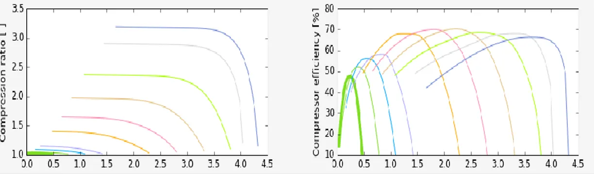
Figure 3. 2: Example of interpolated curves for a compressor. 56
Figure 3. 3: Turbine curves afert data extrapolation. 58
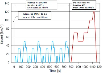
Figure 4. 1: Composition of the NEDC homologation test. 61
Figure 4. 2: WLTC cycle for Class 2 vehicles, with a PMR between 22 and 34.
VIII
Figure 4. 3: Euro emission limits for spark ignition engines. 62
Figure 4. 4: effect of the air/fuel ratio on the NOx production. 63
Figure 4. 5: Example of an EGR (exhaust gas recirculation) system. 63
Figure 5. 1: Alfa Romeo 1.8 TBi engine 65
Figure 5. 2: Engine model into the GasDyn editor. 66
Figure 5. 3: Comparison between experimental and computer perfomances of the engine: the higher ones are the torque curves, and the lower ones
the power curves. 67
Figure 5. 4: Convergence of the compressore and turbine power. 67
Figure 5. 5: Torque at part load compared with the full load curve 69
Figure 5. 6: Engine power at part load compared with the full load curve. 69
Figure 5. 7: Boost pressure at full load and part load. 70
Figure 5. 8: Throttle opening at full load and part load 70
Figure 5. 9: NOx emissions without EGR. 71
Figure 5. 10: GasDyn editor view of the short route EGR. 71
Figure 5. 11: Torque comparison between the three cases. 72
Figure 5. 12: throttle opening angles for the three different layout. 73
Figure 5. 13: target boost pressure for the three different layout. 73
Figure 5. 14: Average NOx emissions on the four cylinders at different EGR
rates. 74
Figure 5. 15: in-cylinder temperatures at 1500 rpm at different recirculation rates
75
Figure 5. 16: in-cylinder temperatures at 2000 rpm at different recirculation
rates. 76
Figure 5. 17: in-cylinder temperatures at 4500 rpm at different recirculation
rates. 76
Figure 5. 18: Long route scheme on GasDyn editor. 77
Figure 5. 19: Boost target pressure for the three main cases. 78
IX
Figure 5. 21: Torque comparison between standard and long route working
points. 79
Figure 5. 22: Compressor working points in the m’rid/compressor ratio plain. 80
Figure 5. 23: Inlet gases temperature at 2000 rpm. 81
Figure 5. 24: Inlet gases temperature at 4500 rpm. 81
Figure 5. 25: NOx emission comparison between long route and short route. 82
Figure 5. 26: In-cylinder temperature at 2000 rpm. 83
Figure 5. 27: In-cylinder temperature at 3500 rpm. 83
X
List of tables
Table 5. 1: Characteristics of the 1.8 TBi engine. 66
Table 5. 2: Mass of fuel injected and spark advance for the investigated regimes
70
Table 5. 3: Difference between real and target recirculation rate. 74
11
CHAPTER 1
GOVERNING EQUATIONS AND
COMPUTATIONAL METHODS
1.1 Governing equations
An internal combustion engine is a cyclic, thermal machine composed by the “proper” engine, made by the cylinders, and the inlet and exhaust ducts that have to bring in and out from the engine the working fluids.
Due to the cyclic behaviour, all the flows that characterize the engine working points are highly unsteady, and so the computation of the fluid proprieties, which are fundamental for evaluating the engine performances requires the solution of very complex differential equations, possible using numerical methods.
These methods need a huge computational power that nowadays is not affordable, so the process is made under the following hypotesis that can lower the computational effort:
• Unsteady flows, • Compressible flows, • One-dimentional flows,
• Low sections variations along the ducts, • Non-adiabatic process,
12 • Non-homentropic process,
• Thermal and friction effects considered only at the boundaries.
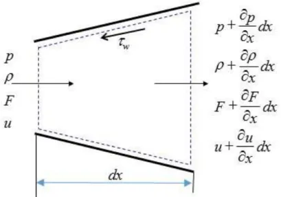
The approach on the definition of the main equations is still differential, but the only dimention considered is now the axial coordinate of the ducts, using an eulerian representation of the flow as showed in figure 1.
Figure 1. 1: One-dimensional approach for the computational process.
We have three fundamental governing equations:
1.1.1
Mass conservation equation
This equation gives the rate of mass change into the control volume, wich is equal to the net mass flow through the element:
𝜕(𝜌𝐹𝑑𝑥)
𝜕𝑡 =
𝜕(𝜌𝑢𝐹)
𝜕𝑥 𝑑𝑥
(1.1)
Where dx is the infinitesima length of a duct, F the cross-sectional area. The derivatives can be expanded, obtaining the following equation:
(𝜌 +𝜕𝜌 𝜕𝑥𝑑𝑥) (𝑢 + 𝜕𝑢 𝜕𝑥𝑑𝑥) (𝐹 𝜕𝐹 𝜕𝑥𝑑𝑥) − 𝜌𝑢𝐹 = − 𝜕(𝜌𝐹𝑑𝑥) 𝜕𝑡 (1.2)
13
Rearranging the terms and considering only the first-order derivatives, the equation is simplified as: 𝜕𝜌 𝜕𝑡 + 𝜌 𝜕𝑢 𝜕𝑥+ 𝑢 𝜕𝜌 𝜕𝑥+ 𝜌𝑢 𝐹 𝑑𝐹 𝑑𝑥 = 0 (1.3)
1.1.2
Momentum conservation equation
This equation keeps in account the fact that the sum of the pressure and shear stress on the boundary of control volume is equal to the rate of increase of momentum of the fluid particle, so we have:
• Pressure contribution, due to the difference of pressure on the end faces and the component on the axial direction of the pressure acting on the sides of the control volume: 𝑝𝐹 − (𝑝 +𝜕𝑝 𝜕𝑥𝑑𝑥) (𝐹 + 𝜕𝐹 𝜕𝑥𝑑𝑥) + 𝑝 𝜕𝐹 𝜕𝑥𝑑𝑥 = − 𝜕(𝑝𝐹) 𝜕𝑥 𝑑𝑥 + 𝑝 𝜕𝐹 𝜕𝑥𝑑𝑥 (1.4)
• The shear stress given by the friction between the moving fluid and the stationary walls that represent the boundaries of the ducts, wich is computed as a “τ∞” stress acting in a direction opposite to the flow:
𝜏𝑤 = 1 2𝜌𝑓𝑢
2 (1.5)
This has to be applied on the entire cross-sectional area, so we find a “friction force” computed as following:
𝐹𝑓𝑟𝑖𝑐𝑡𝑖𝑜𝑛 = −1 2𝜌𝑓𝑢
2(𝜋𝐷𝑑𝑥) (1.6)
• The rate of momentum increase, wich is computed as: 𝜕(𝜌𝑢𝐹𝑑𝑥)
𝜕𝑡 𝑑𝑥 (1.7)
• The net efflux of momentum on the control area: 𝜕(𝜌𝐹𝑢2𝑑𝑥)
14
Keeping in account all these components, the momentum conservation equation can be written as: −𝜕(𝑝𝐹) 𝜕𝑥 𝑑𝑥 + 𝑝 𝑑𝐹 𝑑𝑥𝑑𝑥 − 1 2𝑝𝑢 2𝑓𝜋𝐷𝑑𝑥 =𝜕(𝑢𝜌𝐹𝑑𝑥) 𝜕𝑡 + 𝜕(𝜌𝐹𝑢2) 𝜕𝑥 𝑑𝑥 (1.10)
Then, expanding the derivatives, considering the continuity and re-arranging the equation the following form is found:
𝜕𝑢 𝜕𝑡 + 𝑢 𝜕𝑢 𝜕𝑥+ 1 𝜌 𝜕𝜌 𝜕𝑥+ 𝐺 = 0 (1.11) Where: 𝐺 = 𝑓𝑢 2 2 𝑢 |𝑢| 4 𝐷 (1.12)
1.1.3
Energy conservation equation
This equation is derivaed from the application of the first law of thermodynamics to the control volume, in the form:
𝑄.− 𝑊𝑠. =𝜕𝐸0 𝜕𝑡 +
𝜕𝐻0
𝜕𝑥 𝑑𝑥 (1.13)
The equation can be written using the specific quantities referred to mass, obtaining: 𝜕(𝑒0𝜌𝐹𝑑𝑥) 𝜕𝑡 + 𝜕(ℎ0𝜌𝐹𝑢) 𝜕𝑥 𝑑𝑥 = 𝜕𝑞 𝜕𝑡𝜌𝐹𝑑𝑥 + ∆𝐻𝑟𝑒𝑎𝑐𝑡𝐹𝑑𝑥 (1.14) Where: • 𝑒0 = 𝑒 +1 2𝑢
2, the total specific internal energy;
• ℎ0 = 𝑒 + 𝑝
𝜌, the total specific enthalpy;
• 𝑞 is the heat transfer rate per mass unit;
• ∆𝐻𝑟𝑒𝑎𝑐𝑡 is the reaction hentalpy related to the possible chemical reactions
15
1.1.4
Closure equations
Since the system is composed by three equations bt faces four variables (p, ρ, u, e) there’s the need of another equation that can allow to solve it, wich is represented by the equation of state of the gas flowing in the pipes.
Due to the gas proprieties, the perfect gas equation can be suitable: 𝑝
𝜌= 𝑅𝑇 (1.15)
This equation introduces another variable, the temperature T, but brings back even the benefit that for a perfect gas we can assume than both internal energy and enthalpy are temperature-related, in order to write:
𝑒 = 𝑒(𝑇) = 𝐶𝑣𝑇 (1.16)
And
ℎ = ℎ(𝑇) = 𝑒 + 𝑅𝑇 = 𝐶𝑝𝑇 (1.17)
where Cp, Cv are he specific heat capacities, that have the propriety valid for perfect gas to be written as a ratio wich gives a constant:
𝐶𝑝
𝐶𝑣
= 𝑘 (1.18)
The two specific capacities are also related to the specific gas constant, so it’s possible to write: 𝐶𝑣 = 𝑅 𝑘 − 1 (1.19) 𝐶𝑝 = 𝑘𝑅 𝑘 − 1 (1.20)
This allows finally to write energy and enthalpy as a function of the previous variables and close the system, because the enrgy equation can be written now as:
𝜕 𝜕𝑡[(𝜌𝐹𝑑𝑥)(𝐶𝑣𝑇 + 𝑢2 2] + 𝜕 𝜕𝑥[(𝜌𝐹𝑑𝑥)(𝐶𝑣𝑇) + 𝑝 𝜌+ 𝑢2 2] 𝑑𝑥 = 𝜕𝑞 𝜕𝑡𝜌𝐹𝑑𝑥 + ∆𝐻𝑟𝑒𝑎𝑐𝑡𝐹𝑑𝑥 (1.21)
Wich, combined with the continuity and the momentum equation, gives the following form, where all the products have been solved:
16 (𝜕𝑝 𝜕𝑡 + 𝑢 𝜕𝑝 𝜕𝑡) − 𝑎 2(𝜕𝑝 𝜕𝑡 + 𝑢 𝜕𝑝 𝜕𝑡) − 𝜌(𝑘 − 1) ( 𝜕𝑞 𝜕𝑡 − ∆𝐻𝑟𝑒𝑎𝑐𝑡 𝜌 + 𝑢𝐺) = 0 (1.22) Written in non-conservative form, where:
• a is the speed of sound, function of the gas temperature in homentropic conditions;
After all the system made of hyperbolic equations written in non-conservative formi is the following: 𝜕𝜌 𝜕𝑡 + 𝜕 𝜕𝑥(𝜌𝑢) + 𝜌𝑢 𝐹 𝑑𝐹 𝑑𝑥 = 0 (1.3) 𝜕𝑢 𝜕𝑡 + 𝑢 𝜕𝑢 𝜕𝑥+ 1 𝜌 𝜕𝑝 𝜕𝑥+ 𝐺 = 0 (1.10) (𝜕𝑝 𝜕𝑡 + 𝑢 𝜕𝑝 𝜕𝑡) − 𝑎 2(𝜕𝑝 𝜕𝑡 + 𝑢 𝜕𝑝 𝜕𝑡) − 𝜌(𝑘 − 1) ( 𝜕𝑞 𝜕𝑡 − ∆𝐻𝑟𝑒𝑎𝑐𝑡 𝜌 + 𝑢𝐺) = 0 (1.22) 𝑝 𝜌 = 𝑅𝑇 (1.15) 𝑒 = 𝐶𝑣𝑇 (1.16)
1.1.5
Equations in conservative form
In order to obtain a high level of accurancy of the solutions, th computational process passes through the use of shock-capturing methods, that needs to adopt the equations in their conservative form.
This means that is necessary to identify the variables that remains constant,due to the fact that they’re used for solving the problem around the discontinuities that can emerge in the flow.
So, the system has to be re-written in function of these constant variables, obtaining the following equations set (“strong conservative form”).
𝜕(𝜌𝐹) 𝜕𝑡 + 𝜕(𝜌𝑢𝐹) 𝜕𝑥 = 0 (1.23) 𝜕(𝜌𝑢𝐹) 𝜕𝑡 + 𝜕(𝜌𝑢2𝐹 + 𝑝𝐹) 𝜕𝑥 − 𝑝 𝜕𝐹 𝜕𝑥+ 𝜌𝐺𝐹 = 0 (1.24) 𝜕(𝜌𝑒0𝐹) 𝜕𝑡 + 𝜕(𝜌𝑢ℎ0𝐹) 𝜕𝑥 − 𝜌 𝜕𝑞 𝜕𝑡𝐹 − ∆𝐻𝑟𝑒𝑎𝑐𝑡𝐹 = 0 (1.25)
17
An important advantage of this form is that it can be written even in matrix form, and so the system can be compatted into an only equation as follows:
𝜕𝑤̅(𝑥, 𝑡)
𝜕𝑡 +
𝜕𝐹̅(𝑤̅)
𝜕𝑥 + 𝐵̅(𝑤̅) + 𝐶̅(𝑤̅) = 0 (1.26) Where it can be found the following vectors:
• Conservative variables vector: 𝑤̅ = | 𝜌𝐹 𝜌𝑢𝐹 𝜌𝑒0𝐹 | (1.27) • Fluxes vector: 𝐹̅ = | 𝜌𝑢𝐹 (𝜌𝑢2+ 𝑝)𝐹 𝜌𝑢ℎ0𝐹 | (1.28)
• Source term vector due to the pipe cross-section change: 𝐵̅(𝑊̅ ) = | 0 −𝑝𝑑𝐹 𝑑𝑥 0 | (1.29)
• Source term vector due to fluid friction and heat transfer into the control volume: 𝑐̅(𝑊̅ ) = | 0 𝜌𝐺𝐹 −(𝑞𝜌 + ∆𝐻𝑟𝑒𝑎𝑐𝑡)𝐹 | (1.30)
1.2 Computational methods
The main problem related to the governing equations system is that is non possible to determine a solution for that kind of hyperbolic system by an analytical way.
The solution of these problem passes so through a numerical approximation, and the first studies about that were made by Riemann in 1858, with the developing of the “method of characteristics”, that has been widely used until the ‘80s of the last century, when more accurate “shock-capturing” methods were implemented.
18
1.2.1
Method of charateristics
Therefore actually the most important solving methods are the shock-capturing ones, this method is still used for the modeling of the border conditions of the pipes, despite some limitations due mainly to the following three facts:
• The gas is modeled as a perfect gas with constant specific heat;
• It is a first-order of accurancy method, and the space-time domain is represented into a linearly approximated grid;
• It is not able to recognise discontinuities (shock-waves) into the solution. This method is characterized by the fact that can transfrom partial derivatives into total derivatives, by moving along some partiular lines through the flux, called “characteristic lines”.
As an example, it could be considered an equation in the form:
𝑐 = 𝑐(𝑥, 𝑡) (1.31)
That gives a surface into the (x,t,c) space, considering as a reference c=0.
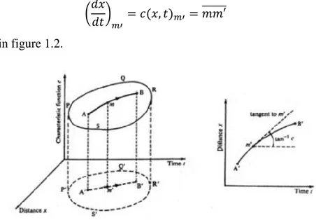
Now, considering a line that connects two points A and B on this surface and its projection on the plan c=0, it can be called “characteristic line” if in every point the slope (angular coefficient) of the projection has the same numerical value of the function in the same point, so that:
(𝑑𝑥
𝑑𝑡)𝑚′ = 𝑐(𝑥, 𝑡)𝑚′ = 𝑚𝑚′̅̅̅̅̅̅ (1.32)
As shown in figure 1.2.
19
This method for the flow computation is based on the equations written in non-conservative form, as follows:
𝜕𝜌 𝜕𝑡 + 𝜕 𝜕𝑥(𝜌𝑢) + 𝜌𝑢 𝐹 𝑑𝐹 𝑑𝑥 = 0 (1.3) 𝜕𝑢 𝜕𝑡 + 𝑢 𝜕𝑢 𝜕𝑥+ 1 𝜌 𝜕𝑝 𝜕𝑥+ 𝐺 = 0 (1.10) (𝜕𝑝 𝜕𝑡+ 𝑢 𝜕𝑝 𝜕𝑡) − 𝑎 2(𝜕𝑝 𝜕𝑡 + 𝑢 𝜕𝑝 𝜕𝑡) − 𝜌(𝑘 − 1) ( 𝜕𝑞 𝜕𝑡 − ∆𝐻𝑟𝑒𝑎𝑐𝑡 𝜌 + 𝑢𝐺) = 0 (1.22)
Combining linearly the three equations it is possible to write them in a form that explicits the three quantities (u+a),(u-a),u.
(𝜕𝑝 𝜕𝑡 + (𝑢 + 𝑎) 𝜕𝑝 𝜕𝑥) + 𝜌𝑎 ( 𝜕𝑢 𝜕𝑡 + (𝑢 + 𝑎) 𝜕𝑢 𝜕𝑥) − (𝑘 − 1)(𝜌𝑞 − ∆𝐻𝑟𝑒𝑎𝑐𝑡+ 𝑢𝐺) + 𝑎2𝜌𝑢 𝐹 𝑑𝐹 𝑑𝑥+ 𝜌𝑎𝐺 = 0 (1.33) (𝜕𝑝 𝜕𝑡 + (𝑢 − 𝑎) 𝜕𝑝 𝜕𝑥) − 𝜌𝑎 ( 𝜕𝑢 𝜕𝑡 + (𝑢 − 𝑎) 𝜕𝑢 𝜕𝑥) − (𝑘 − 1)(𝜌𝑞 − ∆𝐻𝑟𝑒𝑎𝑐𝑡+ 𝑢𝐺) + 𝑎2𝜌𝑢 𝐹 𝑑𝐹 𝑑𝑥− 𝜌𝑎𝐺 = 0 (1.34) (𝜕𝑝 𝜕𝑡 + 𝑢 𝜕𝑝 𝜕𝑥) − 𝑎 2(𝜕𝜌 𝜕𝑡 + 𝑢 𝜕𝜌 𝜕𝑥) − (𝑘 − 1)(𝜌𝑞 − ∆𝐻𝑟𝑒𝑎𝑐𝑡+ 𝜌𝑢𝐺) = 0 (1.35) Then, the equations can be simplified assuming the following “source terms”:
∆1= −(𝑘 − 1)(𝜌𝑞 − ∆𝐻𝑟𝑒𝑎𝑐𝑡+ 𝜌𝑢𝐺) (1.36) ∆2= 𝑎2𝜌𝑢 𝐹 𝑑𝐹 𝑑𝑥 (1.37) ∆3= 𝜌𝑎𝐺 (1.38)
The first and third term are dissipative, so the assume a value higher than zero only in the case of “non-homentropic flow”, so considering friction and heat exchange at the border of the ducts, whereas the second one is conservative because takes in account only the cross-section variation of the ducts.
Now, the “compact form” of the system is the following:
(𝜕𝑝 𝜕𝑡 + (𝑢 + 𝑎) 𝜕𝑝 𝜕𝑥) + 𝜌𝑎 ( 𝜕𝑢 𝜕𝑡 + (𝑢 + 𝑎) 𝜕𝑢 𝜕𝑥) + ∆1+ ∆2+ ∆3= 0 (1.39) (𝜕𝑝 𝜕𝑡 + (𝑢 − 𝑎) 𝜕𝑝 𝜕𝑥) − 𝜌𝑎 ( 𝜕𝑢 𝜕𝑡 + (𝑢 − 𝑎) 𝜕𝑢 𝜕𝑥) + ∆1+ ∆2+ ∆3= 0 (1.40)
20 (𝜕𝑝 𝜕𝑡 + 𝑢 𝜕𝑝 𝜕𝑥) − 𝑎 2(𝜕𝜌 𝜕𝑡 + 𝑢 𝜕𝜌 𝜕𝑥) + ∆1= 0 (1.41)
If the computational process happens on the characteristic lines in the plane (x,t), the terms in brackets will become ordinary derivatives wich proprieties are dependent to the flow ones.
As an example, for the wave propagation velocity into the flow, defined as u+a, the following relationship is valid:
𝜕𝑝(𝑥(𝑡), 𝑡) 𝜕𝑡 = ( 𝜕𝑝 𝜕𝑡 + 𝜕𝑝 𝜕𝑥 𝜕𝑥 𝜕𝑡) = ( 𝜕𝑝 𝜕𝑡 + (𝑢 + 𝑎) 𝜕𝑝 𝜕𝑥) (1.42)
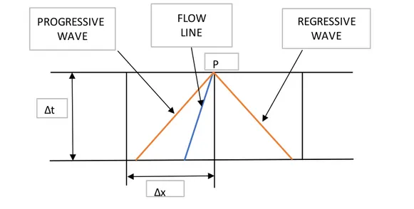
So, the equations that will define the characteristic lines used for transforming the partial derivatives wil be the following, tht are continnous in the (x,t) plan, called “direction equations”: 𝑑𝑥 𝑑𝑡 = 𝑢 + 𝑎, 𝑎𝑏𝑠𝑜𝑙𝑢𝑡𝑒 𝑣𝑒𝑙𝑐𝑖𝑡𝑦 𝑜𝑓 𝑎 𝑝𝑟𝑜𝑔𝑟𝑒𝑠𝑠𝑖𝑣𝑒 𝑤𝑎𝑣𝑒 (1.43) 𝑑𝑥 𝑑𝑡 = 𝑢 − 𝑎, 𝑎𝑏𝑠𝑜𝑙𝑢𝑡𝑒 𝑣𝑒𝑙𝑐𝑖𝑡𝑦 𝑜𝑓 𝑎 𝑟𝑒𝑔𝑟𝑒𝑠𝑠𝑖𝑣𝑒 𝑤𝑎𝑣𝑒 (1.44) 𝑑𝑥 𝑑𝑡 = 𝑢, 𝑓𝑙𝑜𝑤 𝑙𝑖𝑛𝑒 𝑣𝑒𝑙𝑜𝑐𝑖𝑡𝑦 (1.45)
The characteristic lines into the plan are the one that can be graphically represented as shown in figure 1.3, where are written on a discretized (x,t) plan: every characteristic line represents a separation between two different regions of the plan, where we have a discontinuity into the derivated variables but not into the fluid-dynamic ones.
Figure 1. 3:characteristic lines drown into the discretized (x,t) space
Δt
Δx PROGRESSIVE
WAVE
FLOW
LINE REGRESSIVEWAVE P
21
The equations of the system, written on the characteristc lines and so transformed into ordinary derivative ones, are called “compatibility equations”, as follows:
𝑑𝑝 𝑑𝑡+ 𝜌𝑎 𝑑𝑢 𝑑𝑡 + ∆1+ ∆2+ ∆3= 0 (1.46) 𝑑𝑝 𝑑𝑡− 𝜌𝑎 𝑑𝑢 𝑑𝑡 + ∆1+ ∆2− ∆3= 0 (1.47) 𝑑𝑝 𝑑𝑡 − 𝑎 2𝑑𝑢 𝑑𝑡 + ∆1= 0 (1.48)
In order to understand the mechanism, it can be assumed an homentropic case at constant section, where all the three source terms are none, in order to achieve the following equations:
𝑑𝑝 + 𝜌𝑎𝑑𝑢 = 0 (1.49)
𝑑𝑝 − 𝜌𝑎𝑑𝑢 = 0 (1.50)
𝑑𝑝 − 𝑎2𝑑𝜌 = 0 (1.51)
Since the case is hometropic, the two following relations are feasible: 𝑝
𝜌𝑘 = 𝑐𝑜𝑛𝑠𝑡𝑎𝑛𝑡 (1.52)
𝜌
𝑎2/(𝑘−1)= 𝑐𝑜𝑛𝑠𝑡𝑎𝑛𝑡 (1.53)
Then, differentiating both, the equations 1.49 and 1.50 can be transformed as follows:
𝑑𝑢 + 2
𝑘 − 1𝑑𝑎 = 0 (1.54)
𝑑𝑢 − 2
𝑘 − 1𝑑𝑎 = 0 (1.55)
Obtaining the differential of the speed of sound with respect to the flow velocity, wich is: 𝑑𝑎 𝑑𝑢= − 𝑘 − 1 2 (1.56) 𝑑𝑎 𝑑𝑢= + 𝑘 − 1 2 (1.57)
This gives two families of curves, related une to the progressive wave (λ curve) and one to the regressive wave (β curve):
22 𝜆 → { 𝑑𝑥 𝑑𝑡 = 𝑢 + 𝑎 𝑑𝑎 𝑑𝑢= − 𝑘 − 1 2 𝛽 → { 𝑑𝑥 𝑑𝑡 = 𝑢 − 𝑎 𝑑𝑎 𝑑𝑢= + 𝑘 − 1 2
Both of these curves are representable in appropriate graphs, a “position diagram” where are represented the characteristic curves (first equations of the systems) and a “state diagram” where are represented the differential between sound speed and flow velocity, as shown in figure 1.4:
Figure 1. 4: Position and state diagrams for the Riemann variables.
The solution is graphically found in the interception of the two families of curves. Then, is possible to see how, writing the two equations as:
𝑑 (𝑢 + 2
𝑘 − 1𝑎) = 0 (1.58)
𝑑 (𝑢 − 2
𝑘 − 1𝑎) = 0 (1.59)
The two terms into the brakets are constant, due to the fact that the differential is none. This things is possible if we consider an homentropic flow, where the two values are called “Riemann invariants”, whereas in different case they would vary, and then be named as “Riemann variables”.
Riemann invariants 𝐽+ = 𝑢 + 2
23 𝐽− = 𝑢 − 2
𝑘 − 1𝑎 (1.61)
This is finally the correct equation set used by this method.
As a last thing, it is used to adimensionalyze all the variables, in order to define the one that will be used into the proper computational process:
𝐴 = 𝑎 𝑎𝑟𝑒𝑓 , 𝑛𝑜𝑛 − 𝑑𝑖𝑚𝑒𝑛𝑠𝑖𝑜𝑛𝑎𝑙 𝑠𝑝𝑒𝑒𝑑 𝑜𝑓 𝑠𝑜𝑢𝑛𝑑 (1.62) 𝑈 = 𝑎 𝑢 𝑢𝑟𝑒𝑓 , 𝑛𝑜𝑛 − 𝑑𝑖𝑚𝑒𝑛𝑠𝑖𝑜𝑛𝑎𝑙 𝑓𝑙𝑜𝑤 𝑣𝑒𝑙𝑜𝑐𝑖𝑡𝑦 (1.63) 𝐴𝐴 = 𝑎𝐴 𝑎𝑟𝑒𝑓 , 𝑛𝑜𝑛 − 𝑑𝑖𝑚𝑒𝑛𝑠𝑖𝑜𝑛𝑎𝑙 "𝑒𝑛𝑡ℎ𝑟𝑜𝑝𝑖𝑐 𝑠𝑝𝑒𝑒𝑑 𝑜𝑓 𝑠𝑜𝑢𝑛𝑑" (1.64) 𝑍 =𝑎𝑟𝑒𝑓𝑡 𝑥𝑟𝑒𝑓 , 𝑛𝑜𝑛 − 𝑑𝑖𝑚𝑒𝑛𝑠𝑖𝑜𝑛𝑎𝑙 𝑡𝑖𝑚𝑒 (1.65) 𝑋 = 𝑎 𝑥 𝑥𝑟𝑒𝑓 , 𝑛𝑜𝑛 − 𝑑𝑖𝑚𝑒𝑛𝑠𝑖𝑜𝑛𝑎𝑙 𝑠𝑝𝑎𝑡𝑖𝑎𝑙 𝑐𝑜𝑜𝑟𝑑𝑖𝑛𝑎𝑡𝑒 (1.66) The reference values are chosen using “opportune points” for the computational process, that phisically are better explicable looking at the figure 1.5:
Figure 1. 5: a/s diagram for recognizing the value of aref.
It is possible to see that the value of aA is the homentropic speed of sound taken at a
different level of pressure, so applying an homentropic compression or expansion: due to the propriaties of the transformatio, the two following relations are considered valid:
𝑝 𝑝𝑟𝑒𝑓 = ( 𝑎 𝑎𝐴) 2𝑘 𝑘−1 (1.67)
24 𝜌 𝜌𝐴 = ( 𝑝 𝑝𝑟𝑒𝑓) 1 𝑘 (1.68)
In a non-homentropic case the speed of sound will be related to the local enthropy, wich is generally different with respect to the reference one: this has to be taken in account, considering the isobaric enthropy variation:
𝑑𝑠|𝑝 =
𝑑ℎ 𝑇 = 𝐶𝑝
𝑑ℎ
ℎ (1.69)
Then, considering that the hentalpy and its variation can bi written as a function of the speed of sound in the following way:
ℎ = 𝐶𝑝𝑇 = 𝑘𝑅𝑇 𝑘 − 1= 𝑘 𝑘 − 1 𝑝 𝜌 = 𝑎2 𝑘 − 1 (1.70) 𝑑ℎ ℎ = 2𝑑𝑎 𝑎 (1.71)
It is possible to relate the enthropy and the speed of sound: 𝑑𝑠|𝑝 = 2𝐶𝑝𝑑𝑎
𝑎 (1.72)
And so, in a non-homentropic case, the relationship between enthropy and speed of sound can be written in a non-dimensional form as:
𝐴𝐴 = 𝑎𝐴 𝑎𝑟𝑒𝑓 = 𝑒
(𝑠−𝑠𝑟𝑒𝑓)
2𝐶𝑝 (1.73)
Finally, it can be introduced the Riemann invariants: 𝜆 = 𝐴 +𝑘 − 1 2 𝑈, 𝑐𝑜𝑛𝑠𝑡𝑎𝑛𝑡 𝑎𝑙𝑜𝑛𝑔 ( 𝑑𝑋 𝑑𝑍) = 𝑈 + 𝐴 (1.74) 𝛽 = 𝐴 −𝑘 − 1 2 𝑈, 𝑐𝑜𝑛𝑠𝑡𝑎𝑛𝑡 𝑎𝑙𝑜𝑛𝑔 ( 𝑑𝑋 𝑑𝑍) = 𝑈 − 𝐴 (1.75)
That are constant in the case of homentropic flow, and then assume value different from zero in the opposite case, becoming Riemann variables wich variation is the following:
𝑑𝜆 = 𝑑𝐴 +𝑘 − 1
2 𝑑𝑈 (1.76)
𝑑𝛽 = 𝑑𝐴 −𝑘 − 1
25
Thanks to compatibility equations, is possible to evaluate these variations as follows:
λ-characteristic (progessive wave)
Direction equation: (𝑑𝑋 𝑑𝑍) = 𝑈 + 𝐴 (1.78) Compatibility equation: 𝑑𝜆 = −(𝑘−1)(𝐴𝑈) 2 ( 1 𝐹 𝑑𝑓 𝑑𝑋) 𝑑𝑧 − (𝑘−1) 2 2𝑥𝑟𝑒𝑓𝑓 𝐷 𝑈 2 𝑈 |𝑈|[1 − (𝑘 − 1) 𝑈 𝐴] 𝑑𝑍 + (𝑘−1)2 2 𝑞𝑥𝑟𝑒𝑓 𝑎3 𝑟𝑒𝑓 1 𝐴𝑑𝑍 + 𝐴 𝐴𝐴𝑑𝐴𝐴 (1.79)
β-characteristic (progessive wave)
Direction equation: (𝑑𝑋 𝑑𝑍) = 𝑈 − 𝐴 (1.80) Compatibility equation: 𝑑𝛽 = −(𝑘−1)(𝐴𝑈) 2 ( 1 𝐹 𝑑𝑓 𝑑𝑋) 𝑑𝑧 + (𝑘−1) 2 2𝑥𝑟𝑒𝑓𝑓 𝐷 𝑈 2 𝑈 |𝑈|[1 − (𝑘 − 1) 𝑈 𝐴] 𝑑𝑍 + (𝑘−1)2 2 𝑞𝑥𝑟𝑒𝑓 𝑎3 𝑟𝑒𝑓 1 𝐴𝑑𝑍 + 𝐴 𝐴𝐴𝑑𝐴𝐴 (1.81) Path line Direction equation: (𝑑𝑋 𝑑𝑍) = 𝑈 (1.82) Compatibility equation: 𝑑𝐴𝐴 = − (𝑘−1) 2 𝐴𝐴 𝐴2𝑑𝑍 ( 2𝑥𝑟𝑒𝑓𝑓 𝐷 |𝑈 3| +𝑞𝑥𝑟𝑒𝑓 𝑎3 𝑟𝑒𝑓) 𝑑𝑍 (1.83)
Hence, observing the first two compatibility equations, it is possible to see that the variation of the Riemann variables is due to four phenomena:
𝑑(𝜆, 𝛽) = 𝛿𝑠𝑒𝑡𝑖𝑜𝑛+ 𝛿𝑓𝑟𝑖𝑐𝑡𝑖𝑜𝑛+ 𝛿ℎ𝑒𝑎𝑡 𝑒𝑥𝑐ℎ𝑎𝑛𝑔𝑒+ 𝛿𝑒𝑛𝑡ℎ𝑟𝑜𝑝𝑦 (1.84) In the third one the enthropy variation that makes the problem non-homentropic is due only to two components:
26
Considering now the physical meaning of the method of characteristics, it’s known that into a flow the conditions are given by the mass transportation and the pressure perturbations that travel into the ducts at the speed of sound.
In a section i of the duct, at the time t+Δt, the conditions ina certain point called P are due only to the gas states at the previous time t, so from the points C,D,F, as shown in figure 1.6:
Figure 1. 6: the effects on a point P due to the previous conditions in C,D,F
It is possibe to see that the red lines are the characteristic lines, wich slope is dependent from the speed of sound due to the relation given in the direction equations.
Now, the method works in the following way: when the values of the Riemann variables at the time Z (because it is non-dimensional) are known, it is possible to find the enthropy variation using the equation 1.83 (path line).
Then, since the enthropy variation is known, the compatibility equation 1.79 and 1.81 are used to find the Riemann variables variations through the characterstic lines, in order to compute their new value at the time Z+ΔZ, beacuse:
𝜆𝑍+Δ𝑍 = 𝜆 + Δ𝜆 (1.86)
𝛽𝑍+Δ𝑍= 𝛽 + Δ𝛽 (1.87)
Finally, inverting the equations 1.74 and 1.75 is possible to find the soution: 𝐴 =𝜆 + 𝛽
27 𝑈 = 𝜆 − 𝛽
𝑘 − 1 (1.89)
Since this metod has to be applied by a computer, is important to improve a numeric approximated method, called “mesh method od characteristics”.
In this method all the points of intersection of the characterstic lines are defined in the (x,t) plan, such to create a discrete mesh of spatial and temporal positions.
The discretisation happens differently on the two axis:
• Space: this dominion is discretized considering the number of sub-elements in wich the duct is divided: if there are l subelements, there will be l+1 knots. The number of subelements is often chosen as a trade-off between accurancy of the solution and computational effort.
• Time: this dominion is discretized following the Curant-Friedichs-Levy criterion of stability: considering the maximum wave speed propagation u+a, the criterion says that the time step has to be enough short that the wave cannot travel an entire spatial step.
More practically, introducing the CFL number, it has to be: 𝐶𝐹𝐿 = (𝑎 + |𝑢|)Δ𝑡
Δ𝑥 ≤ 1 (1.90a)
𝐶𝐹𝐿 = (𝐴 + |𝑈|)Δ𝑍
Δ𝑋 ≤ 1 (1.90b)
So, in order to have al the knots of the point Z+ΔZ in the right dominion, the CFL number has to be lower than one.
In this mesh method, the computation of the Riemann values for every time step happens only in the spatial knots, in a way represented in figure 1.7:
28
Figure 1. 7: example of computational process in a space/time grid
In order to simplify the computing procedure, acting in a more general way, the two Riemann variables are renamed as λI, λII.
At the adimensional time Z, known the three variables λI, λII, AA, the time step is
computed using the CFL criterion.
Then, the characteristic lines are designed going backwards, so starting from every knot at the time Z+ΔZ and going to time Z, as shown in figure 1.8:
Figure 1. 8: design of the characteristic lines. The path line is the central one, that intersecates the time Z axis in the point s.
The slope of the lines in the graph is constant, whereas in reali it is not: this is so an approximation, and the error introduced is smaller the more the grid is close.
The position of the points P can be computed starting from the values of the two Riemann variables, in the following way (as an example, it is shown the process for the point at the left, but it’s the same for the other):
𝛿𝑋𝐿
Δ𝑍 = 𝑈𝐿+ 𝐴𝐿 (1.91)
29 𝛿𝑋𝐿
Δ𝑍 = 𝑎𝜆𝐼𝐿+ 𝑏𝜆𝐼𝐼𝐿 (1.92)
Where a, b, are two constant that depend from the gas nature: 𝑎 = 𝑘 + 1
2(𝑘 − 1) (1.93)
𝑏 = 3 − 1
2(𝑘 − 1) (1.94)
Now, λI is computed by a linear interpolation using the values of λ in the knots i and
i-1, and similarly λII:
𝜆𝐼𝐿 = 𝜆𝐼𝑖−𝛿𝑋𝐿
Δ𝑋 (𝜆𝐼𝑖− 𝜆𝐼𝑖−1) (1.95)
𝜆𝐼𝐼𝐿 = 𝜆𝐼𝐼𝑖−𝛿𝑋𝐿
Δ𝑋 (𝜆𝐼𝐼𝑖− 𝜆𝐼𝐼𝑖−1) (1.96) And so obtaining the value in function of the interpolated values:
𝛿𝑋𝐿 Δ𝑍 = 𝑎𝜆𝐼𝑖+ 𝑏𝜆𝐼𝐼𝑖 Δ𝑋 Δ𝑍 + 𝑎(𝜆𝐼𝑖− 𝜆𝐼𝑖−1) − 𝑏(𝜆𝐼𝐼𝑖 − 𝜆𝐼𝐼𝑖−1) (1.97)
Once the Riemann variables are known, it is necessary to evaluate the enthropy variation: as provided by the method this is made using the path line compatibility equation, computing the necessary values as an interpolatioon with the next points, with the generic formula:
𝐺𝑠 = 𝐺𝑖−𝛿𝑋𝑠 Δ𝑋 (𝐺𝑖 − 𝐺𝑖−1) (1.98) With: 𝛿𝑋𝑠 Δ𝑋 = 𝜆𝐼𝑖+ 𝜆𝐼𝐼𝑖 Δ𝑋 Δ𝑍 (𝑘 + 1) +(𝜆𝐼𝑖− 𝜆𝐼𝑖−1) − (𝜆𝐼𝐼𝑖− 𝜆𝐼𝐼𝑖−1) (1.99)
When the values of AAS, dAAS are known, it is possible to compute the enthropy of
point P using the relation:
30
Then, the enthropy variation along the characteristic line is:
𝑑𝐴𝐴𝐿 = 𝐴𝐴𝑃− 𝐴𝐴𝐿 (1.101)
Finally, inserting these two values into the equations 1.79 and 1.81, the compatibility equations of the waves, allows to compute the variations Δλ and Δβ, that leads to the evaluation of all the other proprieties.
This method allows to compute the proprieties in all the points of the mesh apart from the first and the last: for the evaluation of the missing Riemann variable are used the border conditions, assumin them in a quasi-steady state that is represented by an algebric equation, so without any derivative term.
Nowadays this method is used only for modeling the border zones.
1.2.2
Shock capturing methods
After the ‘80s of the past century, new and more precise and robut methods for computing the gas flows have been implemented, in order to avoid the problems of low accurancy that affect the method of characteristcs.
These methods are so called due to their capacity to relive the discontinuities into the solution that are given by shockwaves, chemical composition changes and so, and they are based on symmetrical finite differences.
The main problem of these methods come from the fact that they have a “II order of accurancy”, wich brings back the presence of spurious oscillations into the solution that have to be dumped with proper algorithms.
All the most important methods are applied on the hyperbolic system written in the conservative matricial form, the one described in the equation 1.26.
As an example it coud be considered an homentropic case, where the systems becomes as follows:
𝜕𝑤̅(𝑥, 𝑡)
𝜕𝑡 +
𝜕𝐹̅(𝑤̅)
𝜕𝑥 = 0 (1.102)
Then, the Gauss theorem can be applied on the integrated version:
∫ ∫ (𝜕𝑤̅(𝑥, 𝑡) 𝜕𝑡 + 𝜕𝐹̅(𝑤̅) 𝜕𝑥 ) 𝑑𝑥𝑑𝑡 = 0 𝑥+∆𝑥 𝑥 𝑡+∆𝑡 𝑡 (1.103)
31
Since the computational process passes through a numerical approximation, the vector will be “splitted” on all the points of the mesh of the (x,t) grid:
𝑊̅ (𝑥, 𝑡) ≅ 𝑊̅𝑖𝑛(𝑖∆𝑥, 𝑛∆𝑡) (1.104) Such that the equation 1.103 becomes:
(𝑊 ̅̅̅̅ 𝑖𝑛+1− 𝑊̅𝑖𝑛)∆𝑥 + (𝐹̅𝑖+1 2 𝑛 − 𝐹̅ 𝑖−12 𝑛 ) ∆𝑡 = 0 (1.105)
Where the terms are an average on, respectively, space and time:
𝑊̅𝑖 = 1 ∆𝑥∫ 𝑊̅ 𝑥𝑖+1 2⁄ 𝑥𝑖−1 2⁄ 𝑑𝑥 ; 𝐹̅𝑖±1 2⁄ = 1 ∆𝑡∫ 𝐹̅𝑑𝑡 𝑡𝑛+1 𝑡𝑛 (1.106)
The use of the integral average alows to treat discontinuities even without knowing before their precise position.
It’s evident that the equation 1.105 can be written event in the following form:
(𝑊̅𝑖𝑛+1− 𝑊̅𝑖𝑛) ∆𝑡 + (𝐹̅ 𝑖+12 𝑛 − 𝐹̅ 𝑖−12 𝑛 ) ∆𝑥 = 0 (1.107)
In this way it’s possible to do a sum along x and find:
∆𝑥 ∑ 𝑊̅𝑖𝑛+1 𝑖𝑚𝑎𝑥 𝑖𝑚𝑖𝑛 = ∆𝑥 ∑ 𝑊̅𝑖𝑛 + ∆𝑡 𝑖𝑚𝑎𝑥 𝑖𝑚𝑖𝑛 [𝐹̅ 𝑖𝑚𝑖𝑛+12 𝑛 − 𝐹̅ 𝑖𝑚𝑎𝑥−12 𝑛 ] (1.108) Where:
• The first member is the vector W, so the total mass, momentum and energy, at the following time n+1;
• The first term of the second member is the same vector but at the time n; • The second term is the flow of the conserved quantities through the duct sides. The validity of the integral proprieties is due to the conservative scheme adopted.
1.2.3 Lax-Wendroff method
It is based on the Taylor expansion of the vector W, and it’s possible to use it in two different forms: single step or two step.
32
Considering an homentropic case, governed by the equaiton (1.102), it is posible to write it as: 𝜕𝑤̅(𝑥, 𝑡) 𝜕𝑡 + 𝜕𝐹̅(𝑤̅) 𝜕𝑤̅ 𝜕𝑤̅ 𝜕𝑥 = 0 (1.109)
Where the Jacobian matrix A is represented by the first part of the second term:
𝐴 =𝜕𝐹̅(𝑤̅)
𝜕𝑤̅ (1.110)
And its components are expressed as: 𝑎𝑖𝑗 =
𝜕𝐹𝑖
𝜕𝑊𝑗 (1.111)
The equation so can be written even in the following simplified way: 𝜕𝑤̅(𝑥, 𝑡)
𝜕𝑡 + 𝐴
𝜕𝑤̅
𝜕𝑥 = 0 (1.112)
Now, the method requires a Taylor expansion of the vector W in the discretized dominion, wich in the knot i is the following:
𝑤̅𝑖𝑛+1 = 𝑤̅𝑖𝑛+𝜕𝑤̅ 𝜕𝑡|𝑖 𝑛 ∆𝑡 + 1 2! 𝜕2𝑤̅ 𝜕𝑡2| 𝑖 𝑛 ∆𝑡2 + 𝑂(∆𝑡3) (1.113)
Since it is possible to write:
𝜕𝑤̅(𝑥, 𝑡) 𝜕𝑡 = − 𝜕𝐹̅(𝑤̅) 𝜕𝑥 = −𝐴 𝜕𝑤̅ 𝜕𝑥 (1.114)
The second derivative into the equation 1.113 can be rewritten as: 𝜕2𝑤̅ 𝜕𝑡2 = − 𝜕 𝜕𝑡( 𝜕𝐹̅ 𝜕𝑥) = − 𝜕 𝜕𝑥( 𝜕𝐹̅ 𝜕𝑡) (1.115)
So, after some substitutions: 𝜕𝐹̅ 𝜕𝑡 = 𝜕𝐹̅ 𝜕𝑤̅( 𝜕𝑤̅ 𝜕𝑡) = 𝜕𝐹̅ 𝜕𝑤̅(− 𝜕𝐹̅ 𝜕𝑥) = 𝜕𝐹̅ 𝜕𝑤̅(−𝐴 𝜕𝑤̅ 𝜕𝑥) = (−𝐴 𝜕𝐹̅ 𝜕𝑥) (1.116)
Finally, the equation 1.115 becomes: 𝜕2𝑤̅ 𝜕𝑡2 = 𝐴 𝜕 𝜕𝑥( 𝜕𝐹̅ 𝜕𝑥) (1.117)
Now, the relationship found can allow to write the equation 1.113 as an expansion of spatial differences, thanks to the Jacobian matrix:
33 𝑤̅𝑖𝑛+1 = 𝑤̅𝑖𝑛 − 𝐴𝜕𝑤̅ 𝜕𝑥|𝑖 𝑛 ∆𝑡 + 1 2! 𝜕 𝜕𝑥(𝐴 2𝜕𝑤̅ 𝜕𝑥)|𝑖 𝑛 ∆𝑡2+ 𝑂(∆𝑡3) (1.118a) 𝑤̅𝑖𝑛+1 = 𝑤̅𝑖𝑛−𝜕𝐹̅ 𝜕𝑥|𝑖 𝑛 ∆𝑡 + 1 2! 𝜕 𝜕𝑥(𝐴 𝜕𝐹̅ 𝜕𝑥)| 𝑖 𝑛 ∆𝑡2 + 𝑂(∆𝑡3) (1.118b) Then, the derivatives can be substitute with centered finite differences, passing into a discrete dominion, obtaining the one step Lax-Wendroff expressions:
𝑤̅𝑖𝑛+1 = 𝑤̅𝑖𝑛− 𝐴 (𝑤̅𝑖+1 𝑛 − 𝑤̅ 𝑖−1𝑛 2∆𝑥 ) ∆𝑡 + 𝐴2 2! ( 𝑤̅𝑖+1𝑛 − 2𝑤̅𝑖𝑛+ 𝑤̅𝑖−1𝑛 ∆𝑥2 ) ∆𝑡2∆ (1.119a) 𝑤̅𝑖𝑛+1 = 𝑤̅𝑖𝑛 − ∆𝑡 2∆𝑥2(𝐹̅𝑖+1𝑛 − 𝐹𝑖−1𝑛 )∆𝑡 + ∆𝑡2 2∆𝑥2(𝐴𝑖+1 2 𝑛 (𝐹̅ 𝑖+1𝑛 − 𝐹̅𝑖𝑛) − 𝐴 𝑖−12 𝑛 (𝐹̅ 𝑖𝑛− 𝐹̅𝑖−1𝑛 )) (1.119b)
Where the 1.119a is usable when A is constant, and the 1.119b is for the case when A is not constant.
In that situation the values for the jacobian matrix are: 𝐴𝑖±1/2𝑛 = 1 2(𝐴𝑖 𝑛+ 𝐴 𝑖±1 𝑛 ) (1.120a) 𝐴𝑖±1/2𝑛 = 𝐴(𝑊𝑖𝑛+ 𝑊𝑖±1𝑛 ) (1.120b) Whereas this method can be really accurate, it’s not really used due to the high computational effort requested for computing the jacobian matrix into every knot.
Two step method:
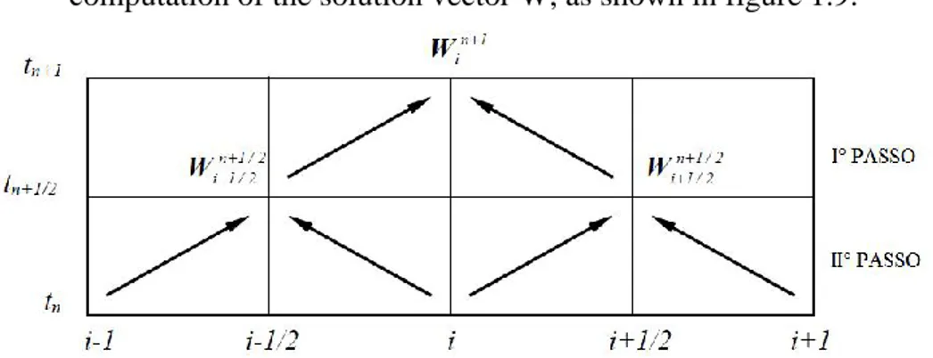
This method allow to not compute the jacobian matrix, using an intermediate computation of the solution vector W, as shown in figure 1.9:
34
• I step: once the vectors W, F are known into the knot i, the previous and the following one, the vector W in the intermediate time n+1/2 is found by a Taylor expansion using finite difference:
𝑤̅𝑖+1/2𝑛+1/2 = (𝑤̅𝑖+1 𝑛 − 𝑤̅ 𝑖𝑛 2 ) − ( 𝐹̅𝑖+1𝑛 − 𝐹̅𝑖𝑛 2∆𝑥 ) ∆𝑡 (1.121a) 𝑤̅𝑖−1/2𝑛+1/2 = (𝑤̅𝑖 𝑛− 𝑤̅ 𝑖−1/2𝑛 2 ) − ( 𝐹̅𝑖𝑛− 𝐹̅𝑖−1𝑛 2∆𝑥 ) ∆𝑡 (1.121b)
• II step: then, it is possible to compute the flow vector F into the intermediate time, and finally compute the solution vector W at the time n+1 in the knot i.
𝑤̅𝑖𝑛+1= 𝑤̅𝑖𝑛 − (𝐹̅𝑖+1/2
𝑛+1/2
− 𝐹̅𝑖−1/2𝑛+1/2
∆𝑥 ) ∆𝑡 (1.122)
The time step is computed using the CFL stability criterium, as the first accurancy order methods.
1.2.4
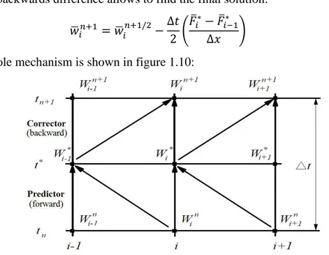
MacCormack method
It’s a two-step method, where the steps are called “predictor” and “corrector”.
Considering the homentropic vectorial equation 1.102 as always, assuming a constant-section duct, the two phases are:
• Predictor phase: once the vectors W, F in time n, it can be computed an approximate version of the solution vector at time t* using forward finite
differences: (𝑤̅𝑖 ∗− 𝑤̅ 𝑖𝑛 ∆𝑡 ) − ( 𝐹̅𝑖+1𝑛 − 𝐹̅𝑖𝑛 ∆𝑥 ) = 0 (1.123a) 𝑤̅𝑖∗ = 𝑤̅𝑖𝑛− Δ𝑡 Δ𝑥(𝐹̅𝑖+1 𝑛 − 𝐹̅ 𝑖𝑛) (1.123b)
Then, even the vector F* can be computed.
The value of the solution vector into an intermediate time step n+1/2 can be computed as an average between the estimated value W* and the previous Win.
𝑤̅𝑖𝑛+1/2= −1 2(𝑤̅𝑖
∗+ 𝑤̅
35
• Corrector phase: concluding the time step by going ahead a time Δt/2, a finite backwards difference allows to find the final solution:
𝑤̅𝑖𝑛+1 = 𝑤̅𝑖𝑛+1/2−Δ𝑡 2 (
𝐹̅𝑖∗− 𝐹̅𝑖−1∗
Δ𝑥 ) (1.125)
The whole mechanism is shown in figure 1.10:
Figure 1. 10: MacCormack forward predictor-backward corrector computational scheme
It is important to remind that the method can be implemented even in the opposite way (backwad predictor-forward corrector), but the results will be a little different.
The best way usually is to follow the discontinuity propagation into the predictor phase, whereas when the direction is unknown a good trade off is to invert the scheme at every step.
The time-step length is still given by the CFL stability criterion.
1.2.5
Spurious oscillations problem
The second accurancy order methods, according with the Godunov theorem, have the problem of a presence of numerical oscilations across the discontinuities of the solution.
In fact, every numerical method above the first accurancy order that can be resumed with the following scheme:
𝑤̅𝑖𝑛+1 = ∑ 𝑐𝑘
𝑘
36
Presents the problem of an oscillating solution, wich has no physical sense.
The sufficient and necessary conditions that a method should have to avoid these oscillations are given by the Hartem criterion: defining the total variation of a solution vector as:
𝑇𝑉(𝑤̅𝑖𝑛) = ∑|𝑤̅𝑖+1𝑛 − 𝑤̅𝑖𝑛|
𝑘
(1.127)
If, going on through the time steps the total variation do not increase, the spurious oscillations problem wil be absent:
𝑇𝑉(𝑤̅𝑖𝑛+1) ≤ 𝑇𝑉(𝑤̅𝑖𝑛) (1.128)
These methods are known as “total variation diminishing”, whereas the two last observed are not into this category.
It is possible to bring them into this category using some damping systems that can modify the ck coefficients, in order to make them dependent from the solution W.
These damping systems can be:
• Pre-processing, if the datas are modified before the solution, so step by step; • Post-processing, if the solution is corrected after all the time steps.
The two systems used by Gasdyn are in the second cathegory, and are: • FCT technique;
• Flux limiters.
FCT technique:
This technique has been introducted in 1973 by Boris and Book, and is constituted by three stages:
• Transport stage, wich is the one where the solution is obtained by a second order method, represented by the transport operator T:
𝑤̅𝑖𝑛+1 = 𝑤̅𝑖𝑛+ 𝑇(𝑤̅𝑖𝑛) (1.129) • Diffusion stage, where a numerical diffusion in introducted in order to damp
any non-physical oscillation by a flux θ: 𝜃̅(𝑤̅𝑖+1/2) =
1
37 𝜃̅(𝑤̅𝑖−1/2) =1
8(𝑤̅𝑖− 𝑤̅𝑖−1) (1.130b)
At wich corresponds the diffusion Di:
𝐷𝑖 = 𝜃̅(𝑤̅𝑖+1/2) − 𝜃̅(𝑤̅𝑖−1/2) (1.131)
Then, there are two possible ways to follow in order to achieve the final value of the solution vector:
1. Damping diffusion, if for the computation of the diffusion factor it is used the vector at time n:
𝑤̅𝐷𝑛+1 = 𝑤̅𝑖𝑛+1+ 𝐷(𝑤̅𝑖𝑛) (1.132) 2. Smoothing diffusion, if the diffusion factor is computed using the solution
vector at the new time n+1:
𝑤̅𝐷𝑛+1 = 𝑤̅𝑖𝑛+1+ 𝐷(𝑤̅𝑖𝑛+1) (1.133) • Anti-diffusion stage, where a counter-diffusive non-linear operator A is
introducted in order to remove the diffusion effects where unnecessary:
𝐴(𝑤̅𝑖𝑛+1) = −𝛹̅(𝑤̅𝑖+1/2𝑛+1 ) + 𝛹̅(𝑤̅𝑖−1/2𝑛+1 ) (1.134) Where the flux limiter ψ is defined using the Ikeda-Nakagawa proposal:
𝛹̅(𝑤̅𝑖𝑛+1) = 𝑠̅ ⋅ 𝑚𝑎𝑥 (0, 𝑚𝑖𝑛 (5 8𝑠̅∆𝑤̅𝑖+1/2 𝑛+1 ,1 8∆𝑤̅𝑖+1/2 𝑛+1 ,5 8𝑠̅∆𝑤̅𝑖+3/2 𝑛+1 )) (1.134) Where: 𝑠̅ = 𝑠𝑔𝑛(∆𝑤̅𝑖+1/2𝑛+1 ) (1.135) ∆𝑤̅𝑖+1/2𝑛+1 = 𝑤̅𝑖+1𝑛+1− 𝑤̅𝑖𝑛+1 (1.136) ∆𝑤̅𝑖−1/2𝑛+1 = 𝑤̅𝑖𝑛+1− 𝑤̅𝑖−1𝑛+1 (1.137) ∆𝑤̅𝑖+3/2𝑛+1 = 𝑤̅𝑖+2𝑛+1− 𝑤̅𝑖+1𝑛+1 (1.138) There are finally two possible values of the damped solution, depending on the strategy followed:
• Damping case:
𝑤̅𝐷𝐴𝑛+1 = 𝑤̅𝐷𝑛+1+ 𝐴(𝑤̅𝑖𝑛) (1.139) • Smoothing case:
38
The difference between this two possibilities is that the damping is more effective in reducing tho spurious oscillations, but makes the numerical process become unstable, whereas the smoothing can mantain the process stable but has lower reduction effect on the oscillation.
A way for limiting the instabilities is to reduce the temporal step lenght, so imposing that the CFL has to be lower than 0.866 instead of 1, wich brings back a higher amount of computational effort.
Flux limiters:
The flux limiters method is based on the idea of applying the diffusion only in the regions where spurious oscillations are present, in order to avoid any non-physical numerical oscillation.
The flux limiter φ can control the oscillations and is function of the ratio between succesive solution’s gradients, defined as:
𝜑𝑖 = 𝜑(𝑟𝑖) (1.141)
Where the ratio is:
𝑟𝑖 =
∆𝑤̅𝑖−1/2𝑛
∆𝑤̅𝑖+1/2𝑛 (1.142)
∆𝑤̅𝑖+1/2𝑛 = ∆𝑤̅𝑖+1𝑛 − ∆𝑤̅𝑖𝑛 (1.143) ∆𝑤̅𝑖−1/2𝑛 = ∆𝑤̅̅̅̅𝑖𝑛− ∆𝑤̅𝑖−1𝑛 (1.144) If the ratio in two adjacent solution is near to one, the second ored accurancy is maintained because there are no oscillations, whereas near the discontiuities the solution is declassated into a forst accurancy order.
On an hyperbolic system the application can be complex, but as an example it is possible to show this method on a linear partial derivative equation like the following:
𝜕𝑤 𝜕𝑡 − 𝑎
𝜕𝑤
𝜕𝑥 = 0 (1.145)
The solution, using the Lax-Wendroff method, is:
𝑤̅𝑖𝑛+1 = 𝑤̅𝑖𝑛+𝜈 2(Δ𝑤̅𝑖+12 𝑛 + Δ𝑤̅ 𝑖−12 𝑛 ) +𝜐2 2 (Δ𝑤̅𝑖+12 𝑛 + Δ𝑤̅ 𝑖−12 𝑛 ) (1.146) Where ν is the CFL.
39
Applying at this equation a dissipative term in order to have an artificial viscosity effect is possible to obtain the TVD propriety for the numerical solution. For example, using a positive constant term it is obtained the following dissipative term:
𝐺𝑖+1/2+ (𝑟𝑖+)𝑤̅𝑖+1/2𝑛 − 𝐺𝑖−1/2+ (𝑟𝑖−1+ )𝑤̅𝑖−1/2𝑛 (1.147) Such that the equation 1.146 becomes:
𝑤̅𝑖𝑛+1 = 𝑤̅𝑖𝑛 − Δ𝑤̅ 𝑖−12 𝑛 {𝜐 [1 +1 2(1 − 𝜐) ( 1 𝑟𝑖+− 1)] − [ 𝐺𝑖+1/2+ 𝑟𝑖+ − 𝐺𝑖−1/2+ ]} (1.148) where: 𝑟𝑖 =∆𝑤̅𝑖−1/2 𝑛 ∆𝑤̅𝑖+1/2𝑛 (1.149) 𝐺𝑖+1/2+ (𝑟𝑖+) =𝜐 2(1 − 𝜐)(1 − 𝜑(𝑟𝑖 +)) (1.150)
In a case of negative constant, the factors are obtained in a similar way:
𝑟𝑖 =∆𝑤̅𝑖+1/2 𝑛 ∆𝑤̅𝑖−1/2𝑛 (1.149) 𝐺𝑖+1/2− (𝑟𝑖−) =𝜐 2(1 − 𝜐)(1 − 𝜑(𝑟𝑖 −− 1)) (1.150)
Then, the two cases can be combined obtaining the following solution:
𝑤̅𝑖𝑛+1 = 𝑤̅𝑖𝑛+𝜈 2(𝑤̅𝑖+1 𝑛 + 𝑤̅ 𝑖−1𝑛 ) + 𝜐2 2 (𝑤̅𝑖+1 𝑛 + 2𝑤̅ 𝑖𝑛 + 𝑤̅𝑖−1𝑛 ) + [𝐺𝑖+1/2+ (𝑟𝑖+) + 𝐺𝑖+1/2− (𝑟𝑖+1− )]Δ𝑤̅ 𝑖+12 𝑛 − [𝐺𝑖+1/2+ (𝑟𝑖−1+ ) + 𝐺𝑖+1/2− (𝑟𝑖−)]Δ𝑤̅ 𝑖−12 𝑛 (1.151) Where: 𝐺𝑖+1/2+ (𝑟𝑖+) = { 𝜐 2(1 − 𝜐)(1 − 𝜑(𝑟𝑖 +)) 𝑖𝑓 𝑎 > 0 0 𝑖𝑓 𝑎 ≤ 0 (1.152a) 𝐺𝑖+1/2− (𝑟𝑖−) = { 0 𝑖𝑓 𝑎 > 0 𝜐 2(1 − 𝜐)(1 − 𝜑(𝑟𝑖 −− 1)) 𝑖𝑓 𝑎 ≤ 0 (1.152b)
Since the sign of the ccoefficient a defines the flow direction, the knowing of that sign is necessary for the solution.
40 𝐺𝑖+1/2+ (𝑟𝑖+) =|𝜐| 2 (1 − |𝜐|)(1 − 𝜑(𝑟𝑖 +)) (1.153) 𝐺𝑖+1/2− (𝑟𝑖−) =|𝜐| 2 (1 − |𝜐|)(1 − 𝜑(𝑟𝑖 +)) (1.154)
In order to make the method TVD, the flux limiter has to assume certain values, defined into the Davis ammissibility region:
𝜑(𝑟) = { 0 𝑖𝑓 𝑟 ≤ 0
min(2𝑟, 1) 𝑖𝑓 𝑟 > 0 (1.155)
41
CHAPTER 2:
INTRODUCTION AND
FUNCTIONING OF GASDYN
2.1 Introduction to GasDyn.
The code used for the simulation of this thesis is GasDyn, wich is a 1-D thermo-fluid dynamic simulator that can represent the whole engine functioning in order to achieve all the informations about volumetric efficiency, torque, power, consumption, emissions and combusion of the engine.
This code can take care of the presence of wave effects into the ducts, and deal with all the devices along the gas path such as valves, volumes, turbines and compressors. The schematics of the engine is easily represented into the main window, as shown in figure 2.1:
42
Inside the cylinders, all the processes are considered using thermodynamic models based on energy conservation equations and mass balance, in the following way.
2.1.1: Instantaneous heat fluxes
The computation of the energy conservation equation needs the evaluation of the instantaneous space averaged heat fluxes, in order to predict the heat transfer between gases and cylinder walls.
There are many sub-models that can decribe the process, whereas the most used is the Woschni approach, wich incudes the effects of radiation into the contribution given by convection, computing the termal power as follows:
𝑞′= ℎ𝑖(𝑇𝑔− 𝑇𝑖) (2.1)
The value of the convective transfer factor h is found using the relationship within the adimensional numbers for forced convection, wich is:
𝑁𝑢 = 𝐶 ∗ 𝑅𝑒0.8 (2.2)
That can be even represented using the variables that constitute the adimensionals: ℎ𝑖𝐷 𝜆 = 𝐶 ∗ ( 𝑢𝜌𝐷 𝜇 ) 0.8 (2.3)
Then, assuming the following proportionalities:
𝜆 ≈ 𝑇0.75 (2.4)
𝜌 ≈ 𝑇−1 (2.5)
𝜇 ≈ 𝑇0.6 (2.6)
And inverting the equation, the following expression is derived:
ℎ𝑖 = 𝐶 ∗ 𝜌0.8∗ 𝐷−0.2∗ 𝑇−0.53∗ 𝑢0.8 (2.7)
Since the real values of the local velocity are generally unknown, the model sees the velocity u as sum of two components, the first considering swirl effects by a constant, the second considering the increase of the velocity during the combustion and expansion process, giving the following expression;
43
Where the two constant are different depending on the engine phase and the paddle wheel speed ωs, and pmot is the in-cylinder pressure of the motored engine (the same
one but without combustion process).
2.1.2 In-cylinder turbulence
The in-cylinder turbulence has a huge effect on the combustion process, so the code has to take them in account during the computation o the combustion: the main used are the K-k models, wich have this name due to the two variables occurring into the two balance equations: the mean motion kinetic energy K and the turbulenct kinetic energy k.
According to the model, the turbulence is generated as a zero-dimensional energy cascade, because the turbulent kinetic energy is generated from the mean one due to viscous dissipation.
Figure 2.2: zero-dimensional energy cascade
The two balance equations that govern the system of production and dissipation of kinetic energy are the following:
𝑑𝐾 𝑑𝑡 = 𝑚′𝑖( 𝑢𝑖 2) 2 − 𝑚′𝑒(𝑢𝑒 2) 2 − 𝑃 − 𝐾 (𝑚 ′ 𝑒 𝑚 ) + 𝑘 ( 𝜌′ 𝜌) (2.9) 𝑑𝑘 𝑑𝑦= 𝑃 − 𝜀 − 𝑘 ( 𝑚′ 𝑒 𝑚 ) + 𝑘 ( 𝜌′ 𝜌) (2.10)
Where is possible to see that the variation fo kinetic energy is due to: • Kinetic energy carried by the massflow entering the cylinder; • Kinetic energy carried outside the cylinder by another massflow; • Kinetic energy carried by the mass moving into the cylinder;
44
• Kinetic energy due to the variation of density acted by the in-cylinder processes as compression or combustion.
It is eviden that only the mean value is affected by the flow going inside or outside the cylinder, whereas for the turbulent component it is interesting the in-cylinder motion. Since the K-k model is not multidimensional, the kinetic energy variations have to be modeled in a phenomenological way: the factors P and ε so are given by the following relations:
𝑃 = 𝐶𝑝(𝐾
𝜏𝑙) (2.11)
𝜀 = 𝐶𝑘(𝐾
𝜏′) (2.12)
Where Cp, Ck are two model constants, τl the integral time scale of large eddies and τ’
the time scale of turbulent eddies.
Assuming the turbulence as homogenoeus and isotropic, at any time step the two velocity component U (mean component) and u’ (mean square root of the velocity fluctuation) a rerelated to the kinetic energy in the following way:
𝐾 =1 2𝑚𝑈 2 (2.13) 𝑘 =3 2𝑚𝑢′ 2 (2.14)
The macroscale of turbulence is assumed as a fraction of the representative scale l: 𝑙𝑙 = 𝐶𝐿𝐼𝑙 = 𝐶𝐿𝐼𝑉
𝜋𝐷2/4 (2.15)
Where V is the instantaneous value of the cylinder volume and D is the cylinder bore. Once this is known, the time scales are computed as turnover time of the fluid in the relative eddies.
45
2.2 Spark ignition engines
2.2.1 Cylinder charge model
The spark ignition combustioni is modeled using a multi-zoe approach, wich is made in the following way.
First of all the in-cylinder mixture is divided into burned and unburned zone, wich are separated by the flame front, assumed as spherical and infinitesimally thin.
In order to have the satisfaction of the momentum conservation, the pressure is assumed as constant.
Therefore, the solution of the mass and energy conservation equations applied in both zones allow computing the pressure and the temperature in the two zones.
The burnt zone can be also divided in more zones, usually from 2 to 4, of equal mass, and are created during the combustion process, as shown in figure 2.3.
All of these sub-zones do not exchange mass by each thers, and are all spherical and centered into the spark plug.
Their chemical composition is computed separately and the same is done with the heat exchange, taking in account the difference of exchanging area of any zone.
This division doesn’t affect the thermodynmical datas determined by the solution of the conservation equations.
Figure 2. 3: multi-zone approach for spark ignition engines.
There will be two kind of sub-zones: burnt ones and the burning one, wich contains the flame front.
46
The two zones are described by different equations as follows: • Burned zone: the energy conservation for this kind of zone is:
𝑑𝐻𝑧 𝑑𝜃 = 𝑑𝑄𝑤,𝑧 𝑑𝜃 + 𝑉𝑧 𝑑𝑝𝑐𝑦𝑙 𝑑𝜃 (2.16)
Where Hz is the hentalpy of the zone, Qw,z is the heat exchanged through the
zone’s walls, Vz is the zone’s volume;
• Burning zone: the temperature is computed using the energy balance applied to the entire volume of burned gases and the zone wich is sub-divided, knwing the mean temperature of the burned gases:
𝑚𝑏ℎ𝑏𝑇𝑏 = ∑ 𝑚𝑖ℎ𝑖𝑇𝑖
𝑁𝑧 𝑖=1
(2.17)
Then, the heat exchange surface is derived by the control volume Vz using the
assumption that each zone is spherical and centered in the spark plug.
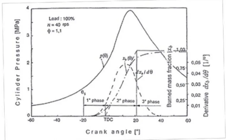
2.2.2 Predicting combustion models
There are more possible models to be used in order to predict the combustion functioning, whereas two are the main important.
• Wiebe function, wich is more simplier and based on a zero-dimensional approach, assuming that the cylinder content has a uniform composition and state at any time, so without any modeling of physical and chemical sub-process as fluid motion, injection, ignition or flame propagation.
The rate of energy release is so represented using quite simple mathematical relations, in order to reproduce the energy release observed by experiments. The Wiebe function represents the burned mass fraction xb using an S-shape
cuve that is function of the crank angle, defined as follows:
𝑥𝑏 = 1 − 𝑒𝑥𝑝 [−𝑎 ( 𝜃 − 𝜃𝑖 𝜃𝑒 − 𝜃𝑖 ) 𝑚+1 ] (2.18)
Where: θi is the actual beginning of combustion, setted a few degreed after the
spark timing, θe is the practical end.
The two parameters a,m are dependent from the geometry of the combustion chamber, and the first is called “efficiency factor” and measures the
47
completeness of the process (for example, for a=6.9 there’s an xb (θe)=0.999,
and for an a=4.6 there’s an xb(θe)=0.99); whereas the second is the “shape
factor” and measures the velocuty of the process in its initial phase, such that the lower m is, the higher will be the initial energy release: this parameter is the one that can be reduced taking in account the effect of phenomenas like the exhaust gases recirculation, assuming generally values between 2 and 5. The variation of the two parameters can bring to obtain a curve that can agree with the experimental datas derived from the pressure measured, as shown in figure 2.4:
Figure 2. 4: Cylinder pressure and bruned mass fraction represented using a Wiebe curve
• Advanced model: if it is necessary to have more complete and accurate results, there’s the need to switch to a more precise model, wich is the advanced ne, characterized by a quasi-dimensional approach.
This model takes in account geometrical features as fluid motions and flame front propagation, wich are added to the thermodynmic equations.
The quasi-dimensional approach is in between 0-D and 1-D, uses phenomenological equations that based on assumptions and relations derived from empirical observations, rather than pure theory.
Once the characteristics of the turbulent field are known there are many models that can predict the evolutioon of the turbulent flame front, using the assumption of Damkoler that the strupture of the turbulent flame can be considered as derived by a lamnar reacting sheet, wich border is wrinkled by turbulent fluid motion.
48
So, a turbulent combustion velocity wtc can be defined as function of the laminar
one wlc (measured by the characteristic chemical reaction velocities) and a main
parameter that takes in account the turbulent levels of reacting gases.
In GasDyn it is employed the Zimont combustion model, wich is simple, robust and able to predict many experimentally observed phenomena using a low number of assumption and constrains, with only two main ideas:
1. in a spark ignition engine, since the fuel is fully vaporized and premixed with air and residual gases, the chemical reactions during the combustion process are slower than the turbulent motions, so the processi s turbulence-controlled; 2. the effects of the different scaled turblences must be treated separately, because
the large eddies distort the flame front, and the small eddies (wich have a scale that is smaller that the flame thckness) intensify the enrgy and mass transfer in the reacting zone.
The number of Damkohler is here used as a measure of turbuence influence on chemical processes, as a ratio between characteristic fluid turnover time in large eddies and characteristic reaction time:
𝐷𝑎 =𝜏𝑡 𝜏𝑙 =
𝑙𝐼𝑡𝑙𝑓
𝑢′𝑤𝑙𝑐 (2.19)
Zimont, using dimensional analisys indications, proposed the following equations for the turbulent combustion velocity:
𝑤𝑡𝑐 = 𝑐𝑧𝑢′𝐷𝑎 1 4 = 𝑐𝑧𝑢′ [( 𝑙𝐼/𝑢′ 𝑡𝑙𝑓/𝑤𝑙𝑐) 1/4 ] (2.20) 𝑤𝑡𝑐 = 𝑐𝑧𝑢′3/4𝑙 𝐼 1/4 𝑤𝑙𝑐1/2𝑥𝑚−1/4 (2.21)
Where cz is an adjustable constant determined from experimental datas and the
laminar front thickness is assumed as proportional to the ratio between thermal diffusivity of the unburned mixture and the laminar combustion velocity:
𝑡𝑙𝑓 = 𝑥𝑚