Testing the methods to reconstruct and model the Baryonic Acoustic Oscillations of different tracers using N-body simulations

(1)

Alma Mater Studiorum - Università di Bologna

Scuola di Scienze

Dipartimento di Fisica e Astronomia

Corso di Laurea Magistrale in Astrofisica e Cosmologia

Testing the methods to reconstruct and model the

Baryonic Acoustic Oscillations

of diﬀerent tracers using N-body simulations

Tesi di Laurea Magistrale

Presentata da:

Giovanni Aricò

Relatore: Chiar.mo Prof.

Lauro Moscardini

Correlatore: Dr.

Federico Marulli

Dr.

Alfonso Veropalumbo

Sessione III

(2)

everyone you ever heard of, every human being who ever lived, lived out their lives on a mote of dust, suspended in a sunbeam. The Earth is a very small stage in a vast cosmic arena. Think of the rivers of blood spilled by all those generals and emperors so that in glory and in triumph they could become the momentary masters of a fraction of a dot. Our posturings, our imagined self-importance, the delusion that we have some privileged position in the universe, are challenged by this point of pale light.”

(3)

“Don’t you hear my call though you’re many years away Don’t you hear me calling you

Write your letters in the sand For the day I take your hand

In the land that our grandchildren knew.”

Queen, ’39, A Night at the Opera (1975)

(4)

(5)

List of Figures

1.1 Concavity of cosmic scale factor . . . 11

1.2 Evolution in redshift of ⌦ . . . 12

1.3 Friedmann Models of the Universe . . . 13

1.4 Geometries of diﬀerent models . . . 16

2.1 Dominant components in the Universe . . . 19

2.2 Evolution of perturbations . . . 24

2.3 Press & Schechter function . . . 27

3.1 Density field decomposition . . . 36

3.2 Bias dependency on the redshift . . . 37

3.3 Models of RSD on the iso-correlation curves . . . 42

3.4 RSD on the iso-correlation curves . . . 44

3.5 Geometrical distortions in the real space . . . 45

3.6 Geometrical distortions in the redshift space . . . 46

5.1 Evolution of a primordial perturbation . . . 55

5.2 CMB Angular Power Spectrum . . . 56

5.3 First BAO detection . . . 59

5.4 Eﬀect of non-linearity on the BAO correlation function . . . 61

5.5 Eﬀect of non-linearity on the BAO . . . 62

5.6 Pictorial BAO reconstruction . . . 63

5.7 BAO reconstruction in the power spectrum . . . 67

5.8 BAO reconstruction in the correlation function . . . 67

5.9 RSD correction with reconstruction . . . 68

5.10 Reconstructed correlation function . . . 68

5.11 BOSS multipoles . . . 77

5.12 BOSS clustering wedges . . . 78

5.13 Cluster correlation functions . . . 78

5.14 Voids correlation functions . . . 79

5.15 BAO in the Ly↵ forest . . . 82

5.16 BAO+CMB probability . . . 83

5.17 Two-dimensional correlation function from BOSS . . . 83

5.18 BAO rings . . . 84

5.19 Consensus constraints in the BOSS survey . . . 85

5.20 The BAO Hubble Diagram . . . 85

6.1 Snapshot of Magneticum simulations Box1mr . . . 91

6.2 Varying rsmooth in the reconstruction . . . 95

(9)

6.3 Reconstruction dependency on rcell . . . 96

6.4 Velocity field vs displacement field . . . 97

6.5 Velocity and displacement mass dependency . . . 98

6.6 Reconstructed 2D correlation function . . . 99

6.7 Comparison between diﬀerent reconstructions . . . 100

6.8 Error estimation . . . 102

6.9 Correlation Matrices . . . 103

7.1 Modelling the galaxy projected correlation function . . . 106

7.2 Modelling the cluster projected correlation function . . . 107

7.3 Modelling the AGN projected correlation function . . . 108

7.4 2 _{test over ⌃} N Lat low redshifts . . . 110 7.5 2 _{test over ⌃} N Lat intermediate redshifts . . . 111 7.6 2 _{test over ⌃} N Lat high redshifts . . . 112

7.7 Correction for non-linear evolution . . . 113

7.8 Modelling the galaxy BAO peak . . . 114

7.9 Modelling the cluster BAO peak . . . 115

7.10 Modelling the AGN BAO peak . . . 115

7.11 Constraints on the ↵ parameter . . . 116

7.12 2 _{test for cluster subsamples . . . .} ₁₁₈

7.13 BAO best-fit models for a cluster subsample . . . 118

7.14 Constraints on ↵ for cluster subsamples . . . 119

7.15 Modelling the BAO using the Box0mr . . . 120

7.16 Reconstruction uncertainties as a function of z . . . 122

List of Tables

1.1 Constraints of Cosmological Parameters from Planck . . . 14

5.1 Results by the BAO analysis of BOSS . . . 77

5.2 Constraints on cosmological parameters from BOSS . . . 80

6.1 Cosmological parameters adopted in the Magneticum simulations . . . 88

6.2 Magneticum simulations Box1mr characteristics . . . 90

6.3 Mean properties of Magneticum catalogues . . . 92

7.1 Results . . . 117 ix

(10)

(11)

Sommario

L’espansione accelerata dell’Universo e la natura dell’Energia Oscura sono tuttora questioni aperte in cosmologia. Realizzare una mappatura su grande scala dell’Universo può aiutare a studiare questi problemi, determinando il tasso di espansione dell’Universo e di crescita delle strutture cosmiche. In particolare, le oscillazioni acustiche barioniche (BAO) propagatesi all’epoca della ricombinazione originano un picco nella funzione di correlazione delle galassie sulla scala caratteristica dell’orizzonte sonoro (rs⇡ 150 Mpc,

una scala suﬃcientemente grande da “proteggere” il segnale dalle forti non linearità), oppure una serie di oscillazioni nello spettro di potenza, la cui lunghezza d’onda è proporzionale a s ' 2⇡/rs. Dato che la scala dell’orizzonte sonoro può essere

determinata con grande precisione dalla posizione del primo picco nello spettro di potenza angolare del fondo cosmico a microonde (CMB, le cui oscillazioni hanno le stesse origini fisiche del BAO, in quanto fino alla ricombinazione vi era un unico plasma di barioni e fotoni), il picco del BAO nella funzione di correlazione delle galassie può essere utilizzato come un “righello standard” per estrarre informazione cosmologica fondamentale, come l’evoluzione nel tempo del parametro di Hubble, H(z), e la distanza angolare DA(z).

Scopo di questa tesi è quello di testare sistematicamente, e possibilmente migliorare, gli strumenti di investigazione statistica utilizzati ad oggi per modellare il picco BAO, tenendo conto dell’evoluzione non lineare delle strutture, delle distorsioni dovute alle velocità peculiari delle galassie e del bias dei traccianti cosmici utilizzati per mappare la materia oscura. Per poter fare questo, abbiamo analizzato cataloghi di galassie, nuclei galattici attivi (AGN) ed ammassi di galassie ottenuti da una delle più grandi simulazioni idrodinamiche cosmologiche disponibili, le Magneticum Simulations (http://www.magneticum.org/), considerando un ampio intervallo di redshift, 0.2  z  2.

Nonostante il picco BAO sia a grandi scale, l’evoluzione non lineare e le velocità peculiari fanno sì che il segnale del BAO sia smussato e allargato rispetto alle predizioni della teoria lineare. in particolare a bassi redshift. La ricostruzione del campo di densità lineare è un metodo per risolvere il problema. Uno degli obiettivi principali di questa tesi è l’implementazione e la verifica di un codice di ricostruzione, analizzando le sue prestazioni in funzione del redshift e degli oggetti cosmici usati come traccianti. La grande maggioranza delle analisi presentate in questo lavoro è stata realizzata tramite le CosmoBolognaLib, una raccolta di librerie C++/Python specificatamente pensata per calcoli cosmologici (Marulli, Veropalumbo, and Moresco,2016).

(12)

Abstract

The accelerated expansion of the Universe and the nature of the Dark Energy are still open questions in cosmology. One of the most powerful ways to investigate these issues is to map the large-scale structure of the Universe, to constrain its expansion history and growth of structures.

In particular, baryon acoustic oscillations (BAO) occurred at recombination make a peak in the correlation function of galaxies at the characteristic scale of the sound horizon (rs⇡ 150 Mpc, a suﬃciently large scale to “protect” the signal from strong

non-linearities), or alternatively a series of oscillations in the power spectrum, whose wavelength is related to s' 2⇡/rs. Since the sound horizon can be estimated with

a great precision from the position of the first peak in the angular power spectrum of the Cosmic Microwave Background (which has the same physical origin of BAO, oscillations of the baryons-photons plasma), the BAO peak in the correlation function can be used as a standard ruler, providing paramount cosmological information, as the redshift evolution of the Hubble parameter, H(z), and the angular distance parameter, DA(z).

The aim of this thesis is to systematically test and possibly improve the state-of-the-art statistical methods to model the BAO peak, taking into account the non-linear evolution of matter overdensities, redshift-space distortions and the bias of cosmic tracers. To do that, we analyse mock samples of galaxies, quasars and galaxy clusters extracted from one of the largest available cosmological hydrodynamical simulations of the standard ⇤CDM model (http://www.magneticum.org/). We extract cosmological constraints from the BAO peak through diﬀerent statistical tools in the redshift range 0.2 < z < 2.

Although the BAO peak is at large scales, non-linear growth and galaxy peculiar velocities make the BAO signal smoothed and broader with respect to linear predictions, especially at low redshifts. A possible method to overcome these issues is the so-called reconstruction of the density field: one of the primary goals of this work is to implement a reconstruction method, to check its performances as a function of sample selections and redshift.

All the analyses presented in this thesis are performed by using the CosmoBolog-naLib, a large set of Open Source C++/Python numerical libraries for cosmological calculations (Marulli, Veropalumbo, and Moresco,2016).

(13)

Introduction

"It is my supposition that the Universe in not only queerer than we imagine, is queerer than we can imagine."

John B. S. Haldane (1892-1964)

At the end of the 19th century there was the conviction that almost everything was discovered in physics. Michelson, especially known for his experiment with Morely to measure the speed of light, and awarded with the Nobel Prize in Physics in 1907, said that “most of the grand underlying principles have been firmly established” and that “the future truths of physical science are to be looked for in the sixth place of decimals”. Philipp von Jolly, professor of Physics in Munich, advised his young student Max Planck not to go into physics, because “in this field, almost everything is already discovered, and all that remains is to fill a few unimportant holes”. These few unimportant holes, probably the same of the “two clouds” which for William Thomson, best known as Lord Kelvin, “obscure the beauty and clearness of the dynamical theory”, are specifically the same Michelson-Morely’s experiment, which couldn’t detect the luminous ether, and the black body radiation eﬀect known as ultraviolet catastrophe.

Well, exactly from these dark clouds, in the earliest years of 20th century, that a young student, Max Planck, and another german-born physicist, Albert Einstein, put the bases of the two most important and most experimentally tested theories of our times, the Quantum Mechanics and the General Relativity (just think about the last confirmed General Relativity’s prediction, the detection of the gravitational waves, B. P. Abbott et al.,2016). Solutions of the Einstein’s equations provide several cosmological models of the Universe: the pure gravitational field equation suggests a dynamical Universe, in contrast with the model accepted at the time; Einstein himself added a term to the equation, the Cosmological Constant ⇤, to describe a static Universe. After Hubble discovery of the Universe expansion, Einstein admitted that the Cosmological Constant was “the biggest blunder of his life”: if he would trust his pure equation, he could "rewind" the space-time expansion developing a Big Bang theory years before that Edwin Hubble measured the recession velocities of spiral galaxies.

Nowadays, in the early years of 21st century, the same equations of General Relativity, together with observational data, tell us that we are really far away from a complete understanding of the reality. With the discovery of the accelerated expansion of the Universe through the study of distant type Ia Supernovae (see Riess et al., 1998), for which Perlmutter, Schmidt and Riess won the Nobel prize in 2011, a lot of open questions arise: which force is driving the expansion? Is gravity diﬀerent on

(14)

large scale? The Cosmological Constant appears again in the equations of the current standard cosmological model, the ⇤ Cold Dark Matter (⇤CDM) model. Independent measurements from distant supernovae, the Cosmic Microwave Background and the large-scale structure of the Universe, attest that the 69% of the content in energy of the Universe is made of Dark Energy, 26% of Cold Dark Matter, 5% of baryons and 10 5_%_{of radiation (P. Ade et al.,}_{2016), where the adjective “dark” is an elegant way}

to say “we really don’t know what it is”. In just a century, we passed from knowing everything excepted for a few holes to knowing only the 5% of the Universe!

With this work we want to take a small step toward the understanding of the nature of the Dark Energy, by testing and possibly improving the modeling of a standard ruler used to constrain paramount cosmological parameters, the Baryonic Acoustic Oscillations (BAO) peaks.

At first time, after the Big Bang, the Universe was hotter and denser than today, the baryonic matter was completely ionized and photons were coupled with baryons through continuos Thomson scattering; Cold Dark Matter, on the contrary, for its low interaction was already decoupled.

Initial fluctuations in the Dark Matter density distribution drove acoustic oscillations of the baryon-photon plasma, trapped in the dark matter gravitational potential. With the expansion of the Universe the temperature of baryons was getting lower, until it was low enough to form first atoms, at the so-called “recombination time” (although it was more properly the first combination of atoms). By consequence there was the baryon-photon decoupling, and the photon waves were free to stream away (technically their mean free path was of the order of the scale of the Universe), but the baryon density waves expanded until the dark matter gravitational attraction made them return into the center of the potential well. Despite of this, we expected a residual overdensity in the matter distribution at the scale of the sound horizon, i.e. the BAO peak, as well as a series of oscillation in the Cosmic Microwave Background (CMB), the first radiation we get from recombination time.

Both oscillations were detected and measured: the BAO peak in the Two-Point Correlation Function of galaxies and galaxy clusters (D. J. Eisenstein, Zehavi, et al., 2005), and the acoustic peaks in the power spectrum of the CMB (Torbet et al.,1999, G. Hinshaw et al.,2007) .

Since we can measure with great precision the scale of the sound horizon from the first peak position in the CMB, we can use the BAO peak position as a standard ruler to constrain the most important cosmological parameters, as the Hubble parameter, in order to understand the expansion history of the Universe and so the nature of the Dark Energy.

The most precise is the BAO detection, the best are the constraints to the cosmological parameters; since non-linearity and peculiar velocities can smooth the BAO peak, technique as the reconstruction of the linear density filed are applied to enhance the signal (D. J. Eisenstein, H.-J. Seo, Sirko, et al.,2007). In this work we test all the techniques and tools to get the best detection of the BAO, using N-body simulations. This work is organized as follow:

The first chapter presents the Einstein’s theory of gravity and discusses the princi-ples on which modern cosmology is based on. It also exposes the main cosmological models.

The second chapter , after a brief exposure of the history of the Universe, shows the cosmological structure formation and growth, exploring both linear and non-linear regime.

(15)

LIST OF TABLES xv The third chapter introduces the clustering of cosmic structures and the main tools

to analyse it, in order to extract cosmological information.

The forth chapter gives a brief introduction to numerical N-body and hydrodynam-ical simulations.

The fifth chapter exposes the Baryonic Acoustic Oscillations theory and the recon-struction technique, showing several observational results.

The sixth chapter after a brief introduction to the Magneticum Simulations, that we have analysed in this work, it exposes in details the methods adopted in the analysis.

The seventh chapter presents and discusses the obtained results.

The eighth chapter gives the conclusions and discusses about the future perspec-tives.

(16)

(17)

Chapter 1

Cosmological Models

“He used to do surgery For girls in the eighties But gravity always wins”

Radiohead, Fake Plastics Trees, The Bends (1995)

Cosmology (from the greek ´o µo& “Universe” and o ´◆↵ “study of”) is the study of the origin, evolution, and fate of the Universe. Studying the Universe as a whole means as a matter of fact studying gravity (excluding the very first moments after the Big Bang), as it is the dominant force on large scales. The strong and the weak interaction, in fact, work on sub-atomic scales and the electromagnetic force, that in theory scales as the inverse of the squared distance exactly as the gravitational force, in practice isn’t eﬀective for the total neutral charge of cosmic bodies.

1.1 Elements of General Relativity

General Relativity (Einstein, 1915) is a geometrical theory: as in the Special Relativity (Einstein,1905), time is not considered as an absolute, but just the forth coordinate of the spacetime. The genial idea of Einstein was to consider gravity not as a force, but as the eﬀect of the geometrical distortion of the spacetime.

In Special Relativity, the separation in spacetime of two diﬀerent events, E1 = (t, x, y, z) and E2 = (t + dt, x + dx, y + dy, z + dz), is defined as

ds2= c2dt2 (dx2+ dy2+ dz2), (1.1) where ds2_{is invariant for coordinate change. The integral over the path of a massive}

particle gives stationary values, so Z

path

ds = 0. (1.2)

In a flat spacetime, as the Minkowski spacetime, this means that the shortest path between two points is a straight line.

(18)

This is no more strictly true in General Relativity, when the spacetime may be curved: we have that

ds2= gijdxidxj, (1.3)

where the indices i and j span between 0 and 3, being x0 _{= ct} _{and x}1,3 _{the space}

coordinates. An interval ds2 _{> 0} _{is called time-like, and ds/c represents the time}

diﬀerence measured by a clock which moves freely between the two points xi _and

xi_{+ dx}_{. A space-like interval is when ds}2_{< 0}_{; it measures the distance between the}

two points from the point of view of an observer at rest. An interval ds2_{= 0}_{is called}

light-like, and it represents the interval which a photon may crosses, from a point xi _to

another xi_{+ dx.}

The metric tensor gij describes the geometry of the spacetime; the shortest path

between two points, called geodesic, for non-Euclidean geometries is not a straight line. The general equation of a geodesic is

d2_xi ds2 + i kl+ dxk ds dxl ds = 0, (1.4) where i

kl is the Christoﬀel symbol, defined as i kl⌘ 1 2g lm  @gmk @xl + @gml @xk + @gkl @xm , (1.5) and gimgmk= ki, (1.6) where i

k is the Kronecker delta.

Starting from Christoﬀel symbols, we can define another tensor which well describes the geometrical properties of the spacetime: the Riemann–Christoﬀel tensor

Riklm⌘ @ i km @xl @ i kl @xm + i nl nkm inm nkl, (1.7)

and the Ricci tensor Rik⌘ Rlilk. The Ricci scalar R ⌘ gikRik gives a measure of the

curvature of the spacetime.

We can now define the Einstein tensor Gik⌘ Rik

1

2gikR. (1.8)

The fundamental equation of Einstein’s gravity may be written as follow: Gik=

8⇡G

c4 Tik, (1.9)

where G is the Universal Gravitational Constant. Tikis the so-called Energy-Momentum

Tensor, which describes the matter distribution for a perfect fluid:

Tik= (p + ⇢c2)UiUk pgik, (1.10)

where p is the pressure, ⇢ is the density and Ui is the four-velocity

Ui = gikUk= gikdx k

ds , (1.11)

xk _{being the spacetime trajectory of the fluid element.}

(19)

1.2. COSMOLOGICAL PRINCIPLES 3 matter-energy distribution.

In the weak gravitational field limit, as we expect, Einstein’s equation returns the Poisson’s equation describing Newton’s gravity,

r2 _{= 4⇡G⇢.} _(1.12)

General Relativity’s field equation, written as above, doesn’t admit a cosmological static solution: as we already told, Einstein added a term to equilibrate the gravity, the Cosmological Constant:

Gik⌘ Rik

1

2gikR ⇤gik= 8⇡G

c4 Tik. (1.13)

Note that we can add the term both in the Einstein tensor or in the Energy-Momentum Tensor: in the first case we modify the properties of the spacetime itself, in the second way we add a component of energy-matter with particular properties, i.e. the Dark Energy.

1.2 Cosmological Principles

General Relativity is one of the most tested physical theory and until now it was confirmed in all the experiments, from the deviation of the light rays in proximity of the sun disk by Sir Arthur Eddington (1919) to the gravitational waves detection by LIGO and Virgo collaborations (B. P. Abbott et al., 2016).

However, it is very hard to solve the Einstein’s field equations to make a completed model of the Universe. Einstein himself and the first cosmologists proposed a principle to simplify the models, specifically the complexity of a general matter distribution, lowering the degrees of freedom of the system with the hypothesis of symmetries of the energy-matter distribution.

In particular, the Cosmological Principle, on which the whole modern cosmology is built, asserts that the Universe is homogenous and isotopic. The homogeneity is the translational invariance, the isotropy the rotational invariance; isotropy does not imply homogeneity without the assumption of not being in a special position of the Universe, the so-called Copernican Principle. According to these principles, the properties of the Universe at suﬃciently large scales should be the same in each point.

Since from General Relativity we know that we are not in a three-dimensional space, but in a four-dimensional spacetime, the Cosmological Principle can be extended to the Perfect Cosmological Principle: the properties of the Universe are the same in all regions, all directions and at all times. This principle was originally formulated by Bondi and Gold (H. Bondi and T. Gold, 1948), and it led Hoyle to develop a steady-state cosmological model, in which the expansion of the Universe was contrasted by a small amount of matter created continuously. This model was later abandoned by the scientific community, after the discover of the Cosmic Microwave Background by Penzias and Wilson (Penzias and Wilson, 1965).

When it was formulated, the Cosmological Principle had not even the smallest obser-vational confirmation, but it was fundamental to lead to simple cosmological models. Nowadays, we know from CMB that that the primordial Universe was isotropic with a precision of one part over 105 _{(Smoot et al.,}_{1992); moreover, the magnitude-distance}

relation of the type Ia Supernovae shows that the Universe is isotropic on the very large scales (Campanelli et al.,2011, Lin et al.,2016); we have also indirect tests of the homogeneity of the Universe (see Heavens et al.,2011). So far, all the observations are in agreement with the Cosmological Principle.

(20)

1.3 The Robertson-Walker metric

Once we assume the Cosmological Principle, from pure geometrical considerations, we get a univocal metric, called the Robertson-Walker metric:

ds2= (cdt)2 a(t)2  _dr2

1 Kr2 + r

2_(d✓2_{+ sin}2_✓d'2_{) ,} _(1.14)

where ✓, ' and r are polar, comoving coordinates. The comoving coordinates are at rest with the Universe expansion: by consequence the comoving distance between two objects does not change with time, not taking account of peculiar velocities of the two objects.

The a(t) parameter is called the expansion parameter or cosmic scale factor: it has the dimension of a length and it is expressed as a function of the proper time t, measured by a clock moving with the object. The curvature parameter, K, could have three diﬀerent values:

• K = 1, the spacetime is a hypersphere: closed, without boundaries but with finite volume;

• K = 0, the spacetime is Euclidean, flat;

• K = 1, the spacetime has a negative curvature, i.e. it is open;

We will see how these three diﬀerent values of K lead to diﬀerent fates of the Universe in the Friedmann cosmological models.

1.4 About Cosmological Distances

In a Universe in which spacetime is expanding, carrying on all its content (Hubble Flow), and the information travels with a finite speed which is at least several order of magnitude smaller than the measurement you’re interest in, it is not easy to define the distance between two points. As a consequence, there is not a univocal definition of distance in cosmology.

• The proper distance, DP, is the distance measured in a hypersurface of constant

proper time (dt = 0), i.e., with a Robertson-Walker metric: DP(r, t) = a(t) Z _dr p 1 Kr2 = a(t)f (r) = a(t) ( sin 1_(r) _{K = 1} sinh 1(r) K = 1 r K = 0 . (1.15)

• The comoving distance, DC, is then the proper distance at present time t0:

DC(r) = a0f (r) = a0

a(t)DP. (1.16)

Proper and comoving distances cannot be directly measured by observations, because the light we received from distant objects travels with a finite speed and so it needs a diﬀerent amount of time to arrive to our telescopes; we cannot therefore make measurements along a surface of constant proper time, but only along the set of light paths travelling to us from the past -our past-light cone (P. Coles and Lucchin, 2002).

(21)

1.5. THE HUBBLE LAW 5 • The luminosity distance,DL, is defined assuming the flux conservation, that is

DL = ✓ _L 4⇡l ◆1/2 = a20 r a, (1.17)

where L is the luminosity of the source, l is the flux received by the observer, r the coordinate distance and a the cosmic scale factor. It is clear from this equation the importance of identifying Standard Candles, objects with known absolute magnitudes, such as Supernovae of type Ia, to measure cosmological distances.

• The angular distance, DA, on the contrary preserves the geometrical properties of

the space, in particular the angular size of an object seen from a certain distance. If D# is the proper diameter of the object and # is the subtended angle, the

angular distance is defined as

DA⌘ a0

D#

# = ar. (1.18)

In this case, it is fundamental to have an object of fixed and known proper diameter, i.e. a “Standard Ruler”. The BAO feature, as we will see, it is a perfect candidate.

A possible way of testing the Robertson-Walker metric is through the duality equation: DA= a(t)r = DL a2 a2 0 ; (1.19)

any consistent violation of this relation would highlight deviations from the assumed homogeneity and isotropy of the Universe. Until now, we have no evidence of deviation from the duality relation.

1.5 The Hubble Law

The proper distance between an observer and any source changes with time, because of the expansion of the Universe: the source will have a radial velocity with respect to the observer

vr=dDP

dt = ˙af (r) = ˙a

aDP. (1.20)

This radial velocity, that Edwin Hubble measured, pointing the Hooker Telescope of Mt. Wilson to a group of spiral galaxies, led him to the discovery of a Universe in expansion, with a velocity proportional to the distance. The equation (1.20) is so called Hubble Law, and the parameter

H(t)_⌘ ˙a

a (1.21)

is called Hubble parameter. The value of the Hubble parameter at the present time is a paramount cosmological information; the last measurement, released from the Planck Collaboration (Planck Collaboration, Adam, et al.,2016), is

(22)

This value expresses the isotropic expansion rate of the Universe, and it is the same in all the space at fixed cosmic time. We can also define the reduced Hubble constant, that is

h_⌘ H0

100Km s 1_Mpc 1 (1.23)

1.5.1 The Deceleration Parameter

The Hubble parameter represents the first derivative of the cosmic scale factor. Expanding a(t) in power series around today, t0, we can see how H(t) varies with the

content of the Universe. Up to the second derivative, we have: a(t) = a0[1 + H0(t t0) 1

2q0H

2

0(t t0)2+ ...], (1.24)

the Deceleration Parameter can then be the defined as: q_⌘ ¨a(t)a(t)

˙a(t)2 , (1.25)

and we will call q0 the present time value of q.

1.5.2 Redshift

The Hubble Law can be used to measure galaxy distances: the radial velocity of galaxies due to the expansion of the Universe causes in fact a measurable redshift in the galaxy spectra.

In the relativistic Doppler eﬀect we have that 1 + z = (1 +vk c ), (1.26) where = ✓ 1 v 2 c2 ◆ 1 . (1.27)

However, until galaxy recession velocities are non-relativistic (v ⌧ c), equation (1.26) can be reduced to

z_⇡vk

c . (1.28)

The redshift is defined as follows:

z⌘ 0 e

e , (1.29)

where e is the wavelength of the radiation emitted by the source and 0 is the

wavelength received by the observer. From equation (1.14), integrating over the path of a light-like interval, it is demonstrated that

a e = a0 0 , (1.30) and then 1 + z = a0 a. (1.31)

(23)

1.6. COSMOLOGICAL MODELS 7 Combining equations (1.20) and (1.28) we can write the Hubble Law, in the non-relativistic limit, as

cz_{⇡ H(z)D}P. (1.32)

Of course, the radial component of peculiar velocities of the galaxies degenerates with the radial velocity due to the expansion of the Universe, so the uncertainty on the distance calculated with the redshift grows-up, as we will discuss in section3.5.1.

Note that the Hubble parameter, H(t), has the dimension of the inverse of time and the deceleration parameter, q(t), is dimensionless. If we combine the equations (1.31) and (1.24), we obtain that

z = H0(t t0) + (1 +

1 2q0)H

2

0(t0 t)2+ ..., (1.33)

which inverted gives

t0 t = 1 H0  z ✓ 1 + 1 2q0 ◆ z2_{+ ... ,} _(1.34)

where t0 is so-called Hubble Time and represents the Universe age (tH⇡ 13.7Gyr).

1.6 Cosmological Models

Combining the Einstein equations (1.9) and (1.10) with the Robertson-Walker metric (1.14), we can derive the two Friedmann equations

¨ a = 4⇡ 3 G ✓ ⇢ +3p c2 ◆ a2 (1.35) ˙a2+ Kc2= 8 3⇡G⇢a 2_. _(1.36)

Solving these two equations, joined to the adiabatic condition, it is possible to describe the expansion of the spacetime. The adiabatic condition is the assumption that the Universe is a closed system: if it doesn’t loose energy, then

dU = pdV, (1.37)

where U = ⇢c2_a3 _{is the internal energy, p is the pressure and V = a}3 _{is the volume.}

The eq. (1.37) can be written also as

d(⇢c2a3) = pda3 (1.38) or equivalently as ˙⇢ + 3⇣⇢ + p c2 ⌘ ˙a a = 0. (1.39)

Note that equations (1.35), (1.36), (1.38) are not independent: from two of these we can determine the third one.

It’s moreover remarkable the Birkhoﬀ’s theorem (1923): any spherically symmetric vacuum solution of Einstein’s equations is locally isometric to a region in Schwarzschild spacetime. The Schwarzschild’s solution of the Einstein field equations describes the geometry of the spacetime around a spherical neutral mass, without any angular

(24)

moment. Its corollary demonstrates that the spacetime inside a homogeneous and isotropic spherical distribution of mass-energy, M, and radius, r, can be described by a Minkowski metric. That is, the spacetime is flat, so we can work in the Newtonian limit, until the condition

GM

rc2 ⌧ 1, (1.40)

is valid.

1.6.1 Einstein Universe

If we recall the first Friedmann equation (1.35), we can note that a static Universe, that is ¨a = ˙a = 0, is possible only if

⇢ = 3p

c2. (1.41)

This means that either the density or the pressure should be negative! To solve this problem, Einstein introduced the Cosmological Constant ⇤ in his field equation (1.13). A similar approach consists in modifying the Energy-Momentum Tensor as follow:

Rik

1 2gikR =

8⇡G

c4 T˜ik, (1.42)

where ˜Tik is obtained by substituting the eﬀective pressure and density, ˜p and ˜⇢, to

preserve the form of the Friedmann equations (1.35) and (1.36): ˜ Tik= pg˜ ij+ (˜p + ˜⇢c2)UiUj= Tij+ ⇤c4 8⇡Ggij, (1.43) where ˜ p = p ⇤c4 8⇡G; ⇢ = ⇢ +˜ ⇤c2 8⇡G; (1.44)

Equations (1.35) and (1.36) are then ¨ a = 4⇡ 3 G ✓ ˜ ⇢ +3˜p c2 ◆ a2 _(1.45) ˙a2_{+ Kc}2₌8 3⇡G˜⇢a 2_. _(1.46)

If we consider a “dust Universe”, where the pressure is negligible (p = 0), we obtain ⇤ = _aK2, ⇢ =

Kc2

4⇡Ga2. (1.47)

The density must be positive, so K = 1 and ⇤ > 0: the Einstein Universe is static (but not stable!) and it is spherical.

1.6.2 De Sitter and Lemaître models

The de Sitter Universe is a model formulated in 1917, in which the Universe is empty and flat (p = 0; ⇢ = 0; K = 0), completely dominated by the Cosmological Constant; from equations (1.44) and (1.46) we have that

˙a2=1 3⇤c

(25)

1.6. COSMOLOGICAL MODELS 9 from which we can note that ⇤ is positive. The solution of the equation (1.48) is

a = A exp "✓ 1 3⇤ ◆1/2 ct # , (1.49)

which gives a Hubble parameter constant in time: H(t) = ˙a a = c ✓_⇤ 3 ◆1/2 . (1.50)

The de Sitter model is actually used to describe the inflationary epoch of the Universe, when for a certain period of time the Universe was exponentially expanding.

The Lemaître Universe is a model formulated in 1927. In this model the parameter of curvature is positive too, and the cosmic scale factor always increases, excepted for a short period in which it results constant (“stagnation”). The stagnation was explaining the apparent surplus of quasars and galaxies at z ⇡ 2 until it was discovered that it was just an apparent eﬀect.

1.6.3 The Friedmann Model

The Russian cosmologist Alexander Friedmann solved the equations (1.35) and (1.36) for a general case, giving the description of the properties of the main cosmological models (Friedmann,1922). He was however almost completely ignored, either because he wrote in german or because he died soon after the publications. The two Friedmann equations depend on three parameters: a(t), p and ⇢; we can add an equation of state to solve the system. When a cosmological component has a particles mean free path smaller than the scale of the cosmic structure physical phenomena, we can describes it as a perfect fluid, that is fully characterised by the following equation of state:

p = w⇢c2, (1.51)

where w is a constant parameter which, in a Universe without any Cosmological Constant, spans the so-called Zel’dovich Interval 0  w  1. The w parameter is linked to the adiabatic sound speed in the fluid as follow:

vs= ✓_@p @⇢ ◆1/2 S = cpw. (1.52)

We can assign at the various components of the Universe the following w parameters: • w = 0, the “dust” case, with p = 0, to describe non-relativistic and non-degenerate

matter; • w =1

3 for ultra-relativistic particles in thermal equilibrium, both not degenerated

matter and radiation;

• w = 1, for the Cosmological Constant equation of state;

The Energy-Momentum Tensor can therefore be written as a sum of diﬀerent compo-nents:

Tµ⌫⌘

X

i

(26)

From equations (1.37) and (1.51) we can get the relation

⇢a3(1+w)= ⇢0wa3(1+w)0 . (1.54)

where the suﬃx “0” indicates, as usual, the parameter measured at present time. We can rewrite the equation (1.36) to highlight the dependence of Robertson-Walker metric’s curvature on the Universe content:

K a2 = 1 c2 ✓_˙a a ◆2✓ ⇢ ⇢c 1 ◆ , (1.55)

where the ⇢c parameter is the critical density

⇢c ⌘

3H2_(t)

8⇡G . (1.56)

If the total density of the Universe is equal to the critical density, then the geometry of the spacetime is Euclidean. We can define also a density parameter

⌦(t)⌘_⇢⇢(t)

c(t)

. (1.57)

We will indicate the density parameter of a single component, having equation of state with w, ⌦w, while the total density parameter will be ⌦tot=Pi⌦wi.

The density parameter provides information on the geometry of the spacetime: • if ⌦tot= 1, the Universe is flat;

• if ⌦tot< 1, the Universe is open;

• if ⌦tot> 1, the Universe is closed;

It is interesting to calculate the time dependencies of cosmological parameters, to study the expansion history of the Universe. Equivalently, we can study how the parameters depend on redshift, because there is a univocal time-redshift relation for a fixed cosmology. From the adiabatic expansion condition (1.37) we can obtain the equation

⇢w(z) = ⇢0w(1 + z)3(1+w), (1.58)

while combining the Hubble Law (1.20) with the Second Friedmann Equation (1.36) we obtain that H2(z) = H02(1 + z)2 " 1 X i ⌦0wi+ X i ⌦0wi(1 + z) 1+3wi # . (1.59) Moreover, from the first Friedmann Equation (1.35) we can get the second derivative of the cosmic expansion parameter

¨ a = 4⇡

3 G⇢(1 + 3w)a. (1.60)

Since we know from observations that H0> 0, and so ˙a > 0, these two equations show

that in a homogeneous and isotropic Universe where w is within the Zel’dovich Interval the cosmic scale factor a(z) grows monotonically with the redshift. As a consequence, as we can see in figure (1.1), there must be an initial singularity, where the cosmic

(27)

1.6. COSMOLOGICAL MODELS 11

Figure 1.1: The cosmic scale factor monotonically increases with the time; the concavity makes the curve crosses the time axis, and so there must be an initial singularity or Big Bang. Figure from (P. Coles and Lucchin,2002).

scale factor is zero and the redshift, the density and the temperature are infinite: the Big Bang cannot be avoided, unless we consider a strong Cosmological Constant, which would introduce a flection point in the cosmic scale factor curve.

If we measure the values of the cosmological density parameters today, we can reconstruct the time evolution of the parameters. Considering just the dominant component in the diﬀerent ages simplifies a lot the calculations: equation (1.59), for example, is reduced to

H2(z) = H02(1 + z)2

⇥

1 ⌦0w+ ⌦0w(1 + z)1+3w⇤, (1.61)

thus from equation (1.58), we have that ⌦w(z) =

⌦0w(1 + z)1+3w

1 ⌦0w+ ⌦0w(1 + z)1+3w

, (1.62)

which can be rewritten as

⌦w1(z) 1 =

⌦01 1

(1 + z)1+3w. (1.63)

This equation, valid for a single component Universe, shows that the geometry of the spacetime cannot change with time: a closed Universe will be always closed, and so a flat or an open one. Moreover, as we can see in Figure (1.2), at high redshift the spacetime tends to the flatness.

Assuming a flat single-component Universe (Einstein - de Sitter Model , hereafter EdS), the equations are even more simplified; for instance, equation (1.61) reduces ulteriorly to

H(z) = H0(1 + z)

3(1+w)

2 ; (1.64)

the various parameters can be determined just substituting the equation-of-state parameter w. Furthermore, it can be shown that

q = 1 + 3w

2 ; (1.65)

this means that an EdS Universe, composed either by matter or by radiation, is in constant deceleration.

(28)

Figure 1.2: Three diﬀerent evolutions of the density parameter ⌦ in redshift; it emerges that the geometry of the spacetime cannot change in time: the curves under and over ⌦ = 1 never cross the line. It is also evident that an open or a closed Universe tend to the flatness with the redshift; this means that to observe today |⌦(t0) 1|  0.01, at the Planck time tP (⇡ 5.39 ⇥ 10 44 s after the Big Bang)

it should be |⌦(tP) 1| = 10 62.

A cosmological model provides information on the past evolution of the Universe, and on the future trend of the cosmological parameters, thus constraining the actual age and fate of the Universe. In figure (1.3) we see how models that have in common the same cosmic scale factor observed today (a0) can have completely diﬀerent origins

and fates (depending also on H0):

• a flat Universe composed only by matter (⌦m= 1) has an age of about 10 Gyr,

and will asymptotically expand until the so-called “heath death” ;

• an open Universe (⌦T < 1) has an age that is greater than a flat Universe, while

its end will be very similar, even if its size per cosmic time will be a little greater; • a closed Universe (⌦T > 1) is younger than a flat Universe. The expansion of the

spacetime will reach a turning point, beyond which there will be a contraction until another singularity, the so-called Big Crunch;

• the ⇤CDM model is a flat Universe, which today is made of 30% of matter and 70%of Cosmological Constant. This Universe has an age of 13.7 Gyr, and the cosmic scale factor presents a flection point; as a consequence, the size of the Universe diverges.

1.6.4 The Standard Cosmological Model

The cosmological model most in agreement with observations nowadays is the flat ⇤CDM model. The main component today is the Cosmological Constant (⇡ 70%), which is driving the accelerated expansion of the Universe. The 25% of the total energy

(29)

1.6. COSMOLOGICAL MODELS 13

Figure 1.3: Diﬀerent evolutions of the cosmic scale factor (i.e. the size of the Universe) as a function of the time, for diﬀerent values of the density factor. The time axis is centered at 0, i.e. today. We can note as all the curves without Cosmological Constant are concave and cross the time axis. As a consequence, in all of these models the Big Bang cannot be avoided. We can also note that the bigger is ⌦m, the younger is our Universe. Closed Universes (⌦m> 1) expands

up to a maximum size, then collapse to another singularity, the so called Big Crunch. As we can see from the dashed line, models with the cosmological constant, even if ⌦T= 1, have a flection point and then diverge. Figure from https://en.wikipedia.org/wiki/Hubble’s_law.

(30)

budget is made by cold dark matter, that is not fully understood yet. Nevertheless, we have several and independent evidences of its existence and some theories on its nature (e.g. Bertone et al.,2005). Only 5% of the energy content of the Universe is made of baryons and radiation. The sum of all the components has, to a very high level of approximation, the value 1 (see Table (1.1)), so the spacetime is flat.

From equation (1.63) it is evident that the distance between ⌦ and the value 1 gets lower with the redshift, as Figure (1.2) shows. At the Planck time tP (⇡ 5.39 ⇥ 10 44

s after the Big Bang), it should be |⌦(tP) 1| = 10 62 to have |⌦(t0) 1|  0.01 at

present time! This apparent fine tuning problem, known as flatness problem, may be resolved by inflationary models1_.

In table (1.1) we resume the values of the main cosmological parameters for the ⇤CDM model, as released from the Planck collaboration, from CMB Power Spectra, plus lensing reconstruction and external data as BAO (P. Ade et al.,2016).

H0 (Km s 1) ⌦⇤ ⌦m Age(Gyr)

67.90_{± 0.55} 0.6935_{± 0.0072} 0.3065_{± 0.0072} 13.796_{± 0.029}

Table 1.1: Cosmological parameters plus best-fit 68% confidence levels, obtained combining data from the Planck Satellite CMB temperature power spectra, data from the reconstruction of lensing and other large-scale structures external data (P. Ade et al.,2016).

1.6.5 Cosmological Horizons

Let us consider a sphere, centered at a generic point of the Universe, with a radius equivalent to the maximum distance from which a signal could have reached that point in the spacetime, that is

RH(t) = a(t)

Z t 0

c dt0

a(t0₎. (1.66)

The distance c dt0 _{travelled by a photon between t}0 _{and t}0_{+ dt}0_{is multiplied by a factor}

a(t)/a(t0₎_{to take into account the expansion of the Universe. If this integral converges,}

this sphere is called particle horizon: all the points inside the particle horizon could in principle have interacted in some way with the center; on the contrary, it is impossible for the central point to receive a signal or any kind of information coming from outside the particle horizon. If the integral diverges, in theory it is possible that this point has received signals from the whole Universe.

For ⌦w= 1, the integral can be approximated to

RH(t)⇡ 3

1 + w

1 + 3wct. (1.67)

In particular, RH(t) = 3ctfor a dust Universe and RH(t) = 2ct for a radiative model.

In the other hand, in a pure de Sitter cosmological model, there is no particle horizon, 1_{see Evrard and P. Coles (}₁₉₉₅_{) for the demonstration that the flatness problem may be only an} apparent fine tuning problem, due to wrong assumptions.

(31)

1.6. COSMOLOGICAL MODELS 15 because the integral of equation (1.66) diverges. Diﬀerent cosmological models have diﬀerent particle horizons, comoving sizes and angles (see Figure (1.4)); measuring the angle that subtends the particle horizon at a time t of known proper size gives information on the spacetime geometry.

It is important not to confuse the particle horizon with the Hubble sphere, or speed of light sphere: its radius, the so-called Hubble radius, is the distance travelled by a particle at the speed of light in the Hubble flow, that is

Rc= ca

˙a = c

H. (1.68)

The Hubble radius can also be seen as the proper distance travelled by light in a Hubble time. It is easy to see that for a flat spacetime it coincides approximately to the particle horizon:

Rc= 3

2(1 + w)ct = 1

2(1 + 3w)RH⇡ RH. (1.69) However, once a point enters the particle horizon, it cannot ever go out of it; the particle horizon at time t takes into account all the past history of the Universe, while the Hubble sphere is defined with the proper distance, so it is instantly defined at a time t. By consequence, a point can be in the particle horizon but not in the Hubble sphere, or can enter in the Hubble sphere, go out and re-enter.

It is interesting to notice that, for the Hubble Law (1.20), points where proper distance is larger than Rc= c/H0 recess with velocities greater than the speed of light.

Observations of the CMB temperature show great homogeneity between points that apparently should be out of each other particle horizons. Inflationary theories explain how physical properties of two points that apparently were never been casually con-nected are so similar (horizon problem) and other issues as the magnetic monopoles problem2_{or the flatness problem, making use of the Hubble spheres.}

Finally, despite it is more used in black hole studies than in cosmology, for completeness we introduce the event horizon, that is the complementary of the particle horizon: it is the sphere that separates the points of the spacetime which could, in principle, emit a signal that can reach the center in a future, from ones which cannot. Its radius is

RE(t) = a(t)

Z tmax

t

c dt0

a(t0₎. (1.70)

Friedmann models with w belonging to the Zel’dovich interval do not have a event horizon, contrary to the de Sitter models.

2 _{GUTs models predict a magnetic monopoles density such that the Universe would be closed,} with a very high density parameter, which is totally in contrast with the observations.

(32)

Figure 1.4: This figure shows how the spacetime geometry of the Universe makes cosmological models diﬀer in angles, horizons and comoving distances. In particular, models of open Universe have larger horizons and distances, but tinier angles; flat models with a Cosmological Constant has larger sizes, but smaller horizons. Figure from (Hamilton,1998).

(33)

Chapter 2

Cosmic Structures

“In the darkness something was happening at last. A voice had begun to sing. Sometimes it seemed to come from all directions at once. There were no words. There was hardly even a tune. But it was, beyond comparison, the most beautiful noise he had ever heard. It was so beautiful he could hardly bear it.”

C.S.Lewis, The Magician’s Nephew (1955)

2.1 Short history of the Universe

Ironically, the Big Bang model describes and predicts well the Universe until a tiny fraction of second before the Big Bang itself: precisely, 10 43 _{seconds, the Planck}

time, before the singularity. Over this time, that is established by the Heisenberg’s indetermination principle, the size of the Universe is small enough to present both quantum and gravitational eﬀects. Nobody was capable to formulate a completely satisfying quantum gravity theory, despite all the tentatives made by the theoretical physicists since Einstein’s times. It is even possible that a quantum gravity theory allows to avoid the primordial singularity, describing the Universe also before the Big Bang, like the loop quantum gravity (e.g. Bojowald, 2008).

The CMB provides a direct evidence that the Universe at z ⇡ 1000 was hotter than now. For this reason the standard cosmological model is also known as Hot Big Bang. It is proved that at high temperature the electromagnetic force is joined to the weak interaction in the so-called electroweak interaction (S. Weinberg,1967); this symmetry is broken at low temperature. There are theories aimed at unifying the strong inter-action (GUTs, Grand Unified Theories) and the gravitational force (supersymmetry theories) to the electroweak force. In some GUT models superheavy (1015_{GeV) bosons}

mediate the unified interaction. The Higgs boson would brake the GUT symmetry; however there are not strong observational evidences for any of these models. The idea that all the fundamental forces are just diﬀerent sides of the same interaction is very attractive, but scientists could not yet formulate the so-called Theory of Everything. The break of a symmetry is called transition phase: during the GUT transition phase, that is when the Universe had a temperature of 1015_{GeV and the strong interaction}

(34)

was separated from the electroweak force, the baryon number was not conserved. This minimum diﬀerence between matter and antimatter could explain the baryogenesis, that is the actual matter-antimatter discrepancy.

About 10 32 _{- 10} 33 _{after the Big Bang, the Universe is believed to have}

experi-enced an instantaneous and exponential expansion called “inflation”. Nowadays there are many inflationary models, originally developed by Alan Guth (A. H. Guth,1981) to solve some main cosmological problems, such as the flatness problem and the horizon problem. It also solves the magnetic monopoles problem and explains the Gaussian anisotropies of the primordial Universe. Moreover, the assumed initial scalar field (inflaton) spontaneously leads to the baryogenesis. The inflationary models, nowadays, are accepted by the largest part of the scientific community, and strongly confirmed by the CMB data from the Planck satellite A. H. Guth et al., 2014. Nevertheless, these models are contested by a few scientists, which consider inflation as a scientific paradigm and claim untestable predictions and lack of empirical evidences (P. J. Stein-hardt,2011; Ijjas et al.,2013; Ijjas et al.,2014).

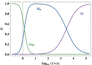
Figure (2.1) shows the redshift evolution of the density parameters. At the beginning, the radiation was the main component of the Universe. After the transition phase period, while the temperature was getting lower, quarks started to bounded into hadrons (the “hadron epoch”), and after about 10 seconds from the Big Bang, during the primordial nucleosynthesis, almost all the hydrogen and helium nuclei of the Universe were formed, with a small percentage of other light elements.

About 47000 years after the Big Bang (z ⇡ 3600), soon after the so-called equivalence time, the matter started to be dominant. Approximatively 380000 years after the Big Bang (z ⇡ 1088), at the recombination time, the Universe had a temperature of ⇡ 4000 K, which is suﬃciently low to start to bind electrons and protons in hydrogen atoms, making the Universe transparent to the radiation (more precisely, “optically thin”). Residual interaction between the matter and photons continued until z ⇡ 400 (matter-radiation decoupling). Later, after the re-heating operated by the luminous

structures, matter and radiation will be locally coupled again.

The matter epoch finished when the Dark Energy started to be the dominant component of the Universe ,“just” 4 billion years ago, about 9,8 billion years after the Big Bang.

2.2 Cosmological Structures Formation

One of the main goals of a cosmological model is to make a link between the past Universe and the present one. The Universe today contains in fact galaxies, clusters, and, on larger scales, filaments and voids. In fact it looks inhomogeneous, at scales of tens Mpc, and it shows eﬀects of the non-linear evolution of its structures. The Universe looks homogeneous today only at the largest scales that can be mapped with the actual surveys, of the order of hundreds Mpc. On the other hand, the Universe at the time of recombination looked smooth and homogeneous as we can see from the CMB light produced 13,7 billions of years ago.

In the Jeans Theory, the structures are formed by the gravitational collapse of small perturbations in a homogeneous mean fluid. Nevertheless, the distribution of photon-matter plasma constrained by the CMB appeared, in the first observations, homoge-neous with a precision of 10 4_{. Eventual anisotropies of the order of 10} 5_{, predicted}

(35)

2.2. COSMOLOGICAL STRUCTURES FORMATION 19

Figure 2.1: Typical behaviours of the density parameters, as a function of the redshift, in Dark Energy cosmological models. The radiation (purple line) was the dominant component for the first 50,000 years after the Big Bang. For most of the time the matter (blue line) was the main component, until the Dark Energy (green line) took its place about 4 billion years ago. Figure from Bamba et al. (2014).

the redshift range ⇡ 2 20 (Zel’dovich, 1972). The discovery of small, Gaussian anisotropies of the order of 10 5 _{in the CMB (Smoot et al.,} _{1992), thus, gave an}

important observational confirmation to the Jeans Theory. At first, we need to define the punctual density contrast:

(x)_⌘ ⇢(x) ⇢¯ ¯

⇢ , (2.1)

where ⇢(x) is the punctual density field, and ¯⇢ is the mean density of the Universe. In the Fourier space, we have that

ˆ(k) = 1 (2⇡)3

Z

d3x (x) eikx, (2.2) where k = 2⇡/x. It is impossible to model the density contrast field exactly, because it is made by stochastic processes. We are interested instead to the statistical information contained in it. Since we have just one Universe from which we can obtain statistical samples, we will work on the hypothesis of Fair Sample: the parts of the Universe suﬃciently distant from each other evolved independently.

The first central moment of the punctual density contrast, that is the mean, is null by construction; if we consider just Gaussian fluctuations, the only non-null moment is the variance: 2 ⌘ _V1 1 Z d3_{x <} 2_{(x) >,} _(2.3)

or equivalently, in the Fourier space:

2

⌘ _(2⇡)13_V 1

Z

(36)

where V1is virtually the volume of the Universe, and the symbol <> means an average

on all the sub-volumes in which the Universe is divided. We can also define the power spectrum , P (k), as

P (k)_⌘< 2(k) > . (2.5) The power spectrum gives a measure of the contribution of a scale k to the total density fluctuation (x); its real-space corresponding quantity is the two-point correlation function, defined as follows:

⇠(r)_⌘ 1 (2⇡)3

Z

d3kP (k)eik·r. (2.6) The power spectrum and the two-point correlation function are linked by the Wiener-Khintchine theorem:

P (k) = Z

⇠(r)eik·rdr. (2.7)

The inflation theory predicts an initial power spectrum of the following form:

P (k) = Akn, (2.8)

where n is the so-called spectral index. Zel’dovich and Harrison proposed independently to set n = 1 (Harrison,1970, Zel’dovich,1970): in this way, the Harrison-Zel’dovich Spectrum has the property to be scale-invariant, and the resultant anisotropies on the CMB are smaller than 10 4 _{, that is the precision achieved at that epoch. The}

observations today provides values consistent with n = 1 (Planck Collaboration, P. A. Ade, et al.,2014), a value that is also predicted by inflationary models. We will discuss more specifically about the two-point correlation functions in the Chapter3.

To compare theory and observations, we need to trace the contrast field in some way. The easiest one is to count luminous objects as galaxies, that constitute a discrete distribution, and to make an average on a given volume. Specifically, for an object of mass M, we have to pick a minimum radius R to have a mean density ¯⇢ / M/R3_{. We}

define the Mass Variance as the convolution of the power spectrum with a window function ˜WR(k), that is used to filter all the information on scales smaller than R:

2 M ⌘ 1 (2⇡)3_V 1 Z d3_{k <} 2_{(k) > ˜}_W2 R(k). (2.9) It is often used 2

8, the mass variance computed with R = 8 h 1 Mpc, for historical

reasons: 2 8⌘ 1 (2⇡)3_V 1 Z d3k < 2(k) > ˜WR=82 (k), (2.10)

in particular, in the galaxy distribution 2

8(z = 0)⇡ 1 .

2.3 Linear theory

Since, as we already discussed in section2.2, CMB temperature fluctuations are of the order of

T T = 10

5_, _(2.11)

we can use the perturbation’s linear theory to describes the initial evolution of the cosmic structures, finding analytical solutions that are valid until (x) < 1.

(37)

2.3. LINEAR THEORY 21 Jeans demonstrated that small density and velocity fluctuations in a homogenous and isotropic mean fluid can grow, accreting mass until the gravitational collapse. The condition for the collapse is simply that the initial perturbation’s length must be larger than a certain scale, called the Jeans Length, J. We can evaluate the forces acting on

a spherical density fluctuation ⇢, of mass M and length , in a homogeneous fluid of mean density ⇢, to have a simple order-of-magnitude idea of the situation:

Fg⇡ GM 2 ⇡ G⇢ 3 2 = Fp⇡ p 2 ⇢3 ⇡ c2 s . (2.12)

The overdense region will collapse if the self-gravitational force per unit of mass, Fg, is

greater than the pressure force per unit mass, Fp, that is if > cs(G⇢) 1/2, where cs

is the speed of sound in the fluid; the Jeans length is then

J' cs

r 1

G⇢. (2.13)

A similar result is achievable by equilibrating the self-gravitational energy, U, of the overdensity with the kinetic energy, K, of the thermal gas, which tends to spread the perturbation,

U _⇡G⇢

3

= K _{⇡ c}2

s, (2.14)

or the gravitational free-fall time, ⌧f f, with the hydrodynamical time, ⌧h:

⌧f f ⇡

1

(G⇢)1/2 = ⌧ h⇡_c s

. (2.15)

If < J, the self-gravity of the overdensity is not suﬃcient for the mass infall in

the gravitational well, and the perturbation propagates as an acoustical wave.

2.3.1 Jeans Theory in a static Universe

We consider here a homogeneous, isotropic, adiabatic and static Universe with time-independent matter density. We can set the following hydrodynamical equation system for a Newtonian, collisional fluid:

Continuity Equation @⇢ @t +r · (⇢v) = 0 (2.16) Euler Equation @v @t + (v· r)v = 1 ⇢r⇢ r (2.17) Poisson Equation r2 _{= 4⇡G⇢} _(2.18) Equation of State p = p(⇢, S) (2.19) Entropy Conservation @s @t + v· rs = 0 (2.20) where ⇢ is the density, v the velocity, the gravitational potential, s the entropy. Once we solved this set of equations for the Universe’s background, we introduce a small perturbation, imposing that the perturbed solutions are still valid; if we look for solutions in the form of plane waves, we get the following dispersion relation in Fourier space:

(38)

where ! is the wave frequency and k is the wave number. In this way we obtain the Jeans length as follows:

J = cs

r _⇡

G⇢. (2.22)

Considering a collisionless fluid, where the particle’s pressure is null, we have to substitute equations (2.16) and (2.17) with the Liouville equation:

@f

@t +r · fv + rv· f ˙v = 0, (2.23) where f is the phase-space distribution function and rV ⌘ (@/@v). The Jeans length

in this case is

J = c⇤

r _⇡

G⇢, (2.24)

where c⇤ replaces the sound speed in equation (2.22):

c_⇤2= R v 2_{f d}3_v R f d3_v ⌘< v 2_{> .} _(2.25)

In particular, for a Maxwellian distribution f (v) = ⇢ (2⇡ 2₎3/2exp ✓ _v2 2 2 ◆ , (2.26)

we have that v⇤= . In a collisionless fluid (as the dark matter one), if the scale of a

perturbation is shorter than the Jeans length, the fluctuation will dissipate in a time of the order of ⌧ ⇡ /c⇤, a process called free streaming, very similar to the Landau

damping in a collisionless plasma.

2.3.2 The Jeans Theory in a Universe in expansion

In an expanding Universe the background density, ⇢B, is not constant, but time

dependent; the peculiar velocities of cosmic structures follow the Hubble Law (1.20). By substituting opportunely these terms in equation (2.16) we get

˙⇢B+ 3H(t)⇢B= 0; (2.27)

we can obtain again a dispersion relation: ¨_k_{+ 2H(t) ˙}_k_{+ (k}2_c2

s 4⇡G⇢b) k= 0. (2.28)

Both the expansion of the Universe, represented by the Hubble friction term 2H(t) ˙k,

and the peculiar velocity field of the fluid, k2_c2

s k, are opposite to the gravitational

collapse of the perturbation. The Jeans length in this case is

J = cs

r _⇡ G⇢B

. (2.29)

These results are valid only on scales inside the particle horizon: outside the horizon, in fact, for the absence of causal connection between particles, there cannot be microphysical processes; only gravitational eﬀects are influent. This means that

(39)

2.3. LINEAR THEORY 23 outside the particle horizon the perturbations always grow due to the absence of the pressure that can oppose the gravitational collapse. Moreover, all the components of the Universe are gravitationally bounded. This means that it is suﬃcient to study only the behaviour of the main component of the Universe at a time t: the other components will follow the dominant one. As already discussed in section 2.1, at first the main component of the Universe was the radiation; after the equivalence it was the matter. Since the dark matter is dominant on the baryonic matter, in an EdS Universe we have that

R/ B/ DM / a(t)2 if z > zeq; (2.30) DM / B/ R/ a(t) if z < zeq; (2.31)

where R, B, DM are fluctuations of radiation, baryons and dark matter

respec-tively, and a is the cosmic scale factor.

Figure (2.2) shows the time evolution of the density fluctuations, in ⇤CDM model. The accretion of an overdensity continue until the scales of the perturbation enter into the particle horizon; the microphysical processes are again effective, and different components behave in different way:

• The radiation fluctuations have a Jeans scale larger than the horizon particle: because of their speed, these fluctuations never collapse, neither before nor after the equivalence time.

• The growth of dark matter fluctuations time is “frozen” before the equivalence due to the so-called Meszaros Eﬀect or stagnation: the lack of the radiation pressure after the equivalence makes the dark matter to collapse again, after the equivalence, with DM / a(t).

• The baryon fluctuations follow the radiation ones, oscillating like acoustic waves until the decoupling, adec; after that epoch, the baryons fall into the dark matter’s

potential wells (baryons catch-up), with B = DM(1 adec/a).

Let + be the density perturbation growing modes in time. It can be demonstrated

that, generically, +(t) = H(t) Z t 0 dt a2_H2_(t) = H(z) Z z 1 (1 + z)dz a2 0H3(z) ; (2.32)

this equation cannot be solved analytically. Nevertheless, in a EdS Universe, where ⌦0,m= 1, through equation (1.64) we can get that

+(z)/ (1 + z) 1/ a. (2.33)

In general, the cosmic structures form faster in closed models, and slower in open ones, relative to a flat Universe, i.e. the higher is the matter content of the Universe, the faster is the growth of overdensities. We can define the linear growth rate parameter as:

f ⌘ d_dln_lna+, (2.34)

It is valid the approximation

f _{⇡ ⌦}m(z) + ⌦⇤ 70 ✓ 1 + 1 2⌦m ◆ ; (2.35)

(40)

where the growth index, , is predicted by the GR, = 0.545 (L. Wang and P. J. Steinhardt,1998a, Linder,2005). Notice that, when the Cosmological Constant, ⇤, is negligible, equation (2.35) reduces to

f _{⇡ ⌦}m(z) . (2.36)

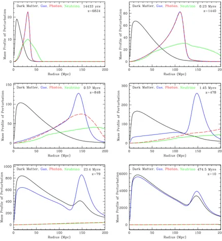
Figure 2.2: Evolution of dark matter (solid line) and baryon (dashed line) perturbations in a ⇤CDM model. Outside the particle horizon all the components are gravitationally bounded and grow together; after entering the particle horizon, the dark matter perturbation keeps growing, while the baryon-photon fluid oscillates. After the decoupling, the radiation keeps oscillating, while the baryons fall in the dark matter wells, in the so-called baryon catch-up. Figure fromhttps://en.wikipedia.org/wiki/Structure_formation.