The Impact of Real Estate and Stock Market
Fluctuations on Human Well-Being
Stefano Castriota
May 2007
Abstract
Fluctuations of house and stock prices have an important effect on household wealth and, consequently, on household consumption patterns. Unfortunately, the recent literature has analyzed the determinants of human well-being and has shown that the relationship between consumption capabilities and happiness is not necessarily linear. In other words, higher income does not automatically imply higher well-being. In this paper I analyze the effects of real estate and stock market fluctuations on self-reported life-satisfaction levels of around 400,000 Western European citizens from 1975 to 2002. There are three main findings. First, both house and stock price increases have a positive effect on happiness. Second, real estate fluctuations are more important than stock market ones, both in relative and absolute terms. Third, when running regressions by age and income subgroups, the coefficients of the two financial variables are always non-negative. Furthermore, low income people are the most sensitive to both stock and house price increases while no big differences emerge among the reaction of different age cohorts. Thus, there does not seem to be room for social conflicts among age cohorts and income groups.
Keywords: real estate, stock markets, life satisfaction, happiness. JEL Codes: E21, E44, I31, R31.
1. Introduction
Over the last years many studies have tried to measure the impact of real estate and stock market fluctuations on wealth and, consequently, on consumption. At the same time a number of other studies have focused on the identification of the socio-economic determinants of well-being: the target of the benevolent social planner/policy maker should be to maximize the population’s welfare, rather than its consumption level per se. Consumption capabilities are only one aspect of human life, although fundamental. Since most of household wealth is held in houses and stocks, it is important to measure the impact of real estate and stock market fluctuations on life-satisfaction, which one is more relevant and what income groups and age cohorts are more sensitive. Policy makers should try to reduce the social conflicts eventually arising among different groups if they display different reactions to such price changes. To my knowledge, this is the first study on the effects of these two sources of wealth on life-satisfaction and on the consequent potential social conflicts arising from market fluctuations.
The paper is organized as follows. Chapter 2 presents a literature review of the effects of real estate and stock market fluctuations on household wealth and consumption (Ch. 2.1) and of the determinants of happiness (Ch. 2.2). Chapter 3 shows the data and the methodology used. Chapter 4 presents the three main empirical results. Chapter 5 concludes.
2. Literature Review
2.1 Real estate and stock market fluctuations, wealth and consumption
Over the last decades a growing body of literature has analyzed the effects of asset markets on consumption. Housing is the dominant component of wealth for the typical household in the United States and Europe, while financial assets follow closely. Real estate and stock market fluctuations can strongly influence upward or downward household financial wealth, like the dot-com stock market boom until 2000 and the real estate bubble of the last years. Therefore, it is reasonable to expect some effect on household consumption.
The nature of the effect on consumption has to be analyzed in a permanent income/life-cycle perspective (see Friedman, 1957 and Ando and Modigliani, 1963). There are two main transmission channels: liquidating assets and borrowing capacity. The first is more relevant for stock markets, given their intrinsic higher liquidity: selling an asset after a price boom provides a capital gain which increases the permanent income and allows higher consumption levels. Unexpected wealth shocks change the household permanent income, thereby affecting the life-cycle pattern of saving and consumption (see Lettau and Ludvigson, 2004). The second refers mainly to real estate markets: housing properties can be used as collateral to weaken the borrowing constraints towards financial
institutions and increase the consumption level. Agents want to smooth consumption over their life-cycle, thus they will distribute over time the increases in anticipated income or wealth. Both assets have advantages: stocks are liquid and can easily be sold to monetize the gain or minimize the loss, while houses can be used as collateral and their prices are more stable.
On the other hand, from a theoretical point of view the overall wealth effect on consumption is not necessarily unambiguous, especially for the real estate market. A substantial percentage of financial assets are held into unquoted shares or private pension and investment funds which cannot be sold whenever one believes the price to be convenient. More importantly, capital gains from increased real estate prices imply also higher costs for housing services like rental costs and mortgage repayments for non-homeowners. Households planning to buy a new house or to move to a bigger one will have to reduce their consumption level to save more for down-payments and repayments. Hence, some or all of any consumption increases made by current owners might be offset by increased savings of renters who aspire to become homeowners as mentioned, among others, by Englund and Yoannides (1997). Finally, focusing on the wealth effect (without considering the effect on collateral and credit), homeowners can increase their consumption level only if they reduce their consumption of housing services. In other words, homeowners who are not planning to sell a house (e.g. because they are currently living there and are not planning to move to a smaller one) are only theoretically, but not actually richer.
However, most of empirical studies show that the wealth effect of both stock and the housing markets on consumption is positive. Evidence of a positive housing effect on consumption has been found by Skinner (1989) for the U.S., Yashikawa and Ohtake (1989) for Japan, Case (1992) for New England, Brodin and Nymoen (1992) for Norway, Koskela et al. (1992) for Finland, Bayoumi (1993) for the U.K., Engelhardt (1994) for Canada, Berg and Bergström (1995) for Sweden, and others. Using data from the PSID during the 1980s Engelhardt (1996) finds that the link between house price appreciation and savings behavior of US homeowners under age 65 derives from an asymmetry in the saving response. Households that experience real losses reduce their consumption levels while households that experience real gains do not modify their behavior.
A natural question is: which of the two effects is more important? The answer depends on whether we compare relative or absolute effects. If we compare the marginal propensity to consume (relative impact) of the two variables there is more evidence suggesting a higher MPC for housing than for financial wealth. An early paper by Elliot (1980) finds a positive effect of financial wealth while “houses, automobiles, furniture and appliance can be treated more as part of the environment by households than as a part of realizable purchasing power” (p. 528). However, the method used to estimate non-financial wealth is questioned by Bhatia (1987). Dvornak and Kohler (2003), using a panel of Australian states, find a MPC equal to 0.03 for housing wealth and equal to 0.06-0.09 for financial wealth. Boone and Girouard (2002), analyzing aggregate data on six of the G7 countries,
with the exception of Germany1, find a positive effect of both forms of wealth on consumption, although results are not easy to compare.
On the other hand Levin (1998), with survey data from the Retirement History Survey, finds a MPC of 0.5-0.6 for housing wealth and less than 0.02 for financial wealth. Benjamin, Chinloy and Jud (2004), using U.S. aggregate quarterly data from 1952 to 2001, find that an additional dollar of housing wealth increases consumption by 8 cents, compared with only 2 cents for financial wealth. Consequently, the marginal propensity to consume (MPC) out of housing wealth is four times the size of that from financial assets. Bostic, Gabriel and Painter (2005), using U.S. micro data from the Survey of Consumer Finance and from the Consumer Expenditure Survey over the period 1989-2001, find that housing wealth elasticities range from 0.063 in 1989 to 0.057 in 1989-2001, while financial wealth elasticities range from 0.021 in 1989 to 0.015 in 2001. Although both forms of wealth seem to become less important over time, this result is in line with Benjamin, Chinloy and Jud (2004): real estate wealth is three up to four times more important. Case, Quigley and Shiller (2005), using two different panel datasets for European countries and U.S. states, find a statistically significant and rather large effect of housing wealth upon household consumption.
Another relevant issue refers to the size of the wealth effects at different age cohorts. While the MPC out of financial wealth is expected to be a function of the households’ total income and wealth, in the case of housing wealth there can be significant redistribution effects between agents at different stages of their housing career2. Rising prices redistribute income away from new entrants towards households about to leave the owner-occupancy market. Usually young people start living in small apartments, then move to bigger houses when the size of the family grows, finally (sometimes) move back to smaller places when children leave. Following this line of reasoning, we should be able to observe older homeowners increasing their consumption when house prices rise, while young renters should cut their consumption. Quite consistently, Campbell and Cocco (2005) using data on the U.K. find a strong positive effect of house prices on consumption for older homeowners and no effect for younger renters. The authors argue that this latter result is due to the fact that households tend to substitute non-durable consumption for housing consumption, thus counteracting the negative wealth effect. Lehnert (2004) estimates consumption elasticities from housing wealth by age quintile. The result is that the youngest group has higher elasticity of consumption than the next two age quintiles. The elasticity of the quintile about to retire is the highest, then diminishes although remains positive. The author claims, in a life-cycle perspective, that the youngest want to consume more since they have the highest permanent income increases. They would like to borrow, but are liquidity-constrained. Higher house prices relax their borrowing constraints, no matter if they move to a bigger house in the future and have to pay a higher price for this. People about to retire have the highest elasticity
1 Germany was not included in the sample because housing wealth was not available over a long enough
period for econometric analysis.
2
In other words, there is no reason to expect a negative effect of stock market rises for any age cohorts. On the contrary, rising house prices might benefit old age cohorts and damage young ones.
because they have accumulated housing wealth for the entire life and are probably going to move to a smaller place, realizing substantial capital gains. Finally, the elasticity of the oldest people (above age 62) is still positive because, if they move to a smaller place, the capital gain might help to compensate the lower income due to retirement.
Even if, to some extent, the results of some studies seem to be sample-specific (which is often the case), when taking into account the composition of the households’ wealth it generally appears that housing wealth has a stronger absolute effect on savings and consumption than financial wealth. This might be due to the fact that a higher share of household wealth is held in real estate form. Norman, Sebastia-Barriel and Weeken (2002) calculate that in the first three quartiles of the income distribution of Italy, France, Germany, U.K. and U.S., less than 20 percent of the population owns shares. As noted by Boone and Girouard (2002), this is important since the agents with the largest propensity to consume out of wealth are typically considered to be those with lower wealth holdings and lower income. Most of financial assets are held by big private equity and pension funds and by a minority of wealthy households. On the contrary, the majority of American and (especially Southern) European families are homeowners. Consequently it is normal to expect a higher absolute impact of real estate fluctuations on consumption patterns.
2.2 The determinants of happiness
Although the theoretical discussion on the role of happiness in economics has become increasingly popular since Easterlin’s (1974) seminal paper, there is plenty of social scientists and philosophers who, over the centuries, speculated about the importance and the pursuit of happiness. As an example, it is worth to mention this nice quote from Malthus (1798) on Adam Smith’s work: “The professed object of Dr. Adam Smith’s inquiry is the nature and the causes of the wealth of nations. There is another inquiry, however, perhaps still more interesting, which he occasionally mixes with it, I mean an inquiry into the causes which affect the happiness of nations”.
As previously written, the first rigorous economic paper on happiness has been written by Easterlin (1974), whose purpose was to study the relationship between income and life-satisfaction over time and across countries. His surprising result was that “money does not buy happiness”: higher per capita GDP levels do not automatically imply higher average happiness scores. The author showed that in 1960 some African and South American countries had much lower GDP per capita but same or even superior average well-being than Germany. Furthermore, the average life-satisfaction of American citizens in the post WWII period was found to be almost constant while the real GDP per capita had doubled or tripled.
The literature on the link between real personal income and happiness has grown a lot over the last decades and has benefited a number of important academic contributions. Veenhoven (1993) with data on Japan, Oswald (1997) with data on the U.S. and Europe and Blanchflower and Oswald (2004) with data on the U.S. and U.K., confirm Easterlin’s (1974) results, while Diener and Oishi (2000) with data on Denmark, Germany and Italy
provide a counterexample. Castriota and Van Horn (2007), using country-average time-series data on sixteen Western European countries from the Eurobarometer3, conclude that no general rule exists since the pattern can be positive, null or even negative. Instead, using simple pooled cross-section data on 72 countries from the World Bank’s World Value Survey4, they find support for a strong non-linear relationship between real PPP per capita GDP and happiness, which is in line with the findings in Frey and Stutzer (2002).
Much effort has been put to solve this puzzle and explain why higher income does not automatically increase life-satisfaction by the same amount. The most obvious theory refers to the diminishing marginal utility of absolute income, since initial income is used to purchase primary goods which have a stronger impact on individuals’ well-being. Adaptation effects play an important role: people increase their income aspirations over time because they get used to higher standards of living. When we had 100 $ we though that 200 $ would have made us very satisfied, but after a while we will get used to the 200 $ and will consider 400 $ the necessary amount to make us very happy.
Many studies have stressed the importance of relative rather than the absolute income. People compare themselves with others, thus well-being increases with own income and decreases with others’ one. The consciousness of belonging to the richest share of the population is as important as being wealthy, or possibly even more. We are more likely to be very satisfied of the quality of our life if we have 100 $ and our neighbor 50 $ rather than when we have 100 $ and our neighbor 200 $. Consequently, if the per capita GDP rises over time but the income distribution is identical, the marginal utility of additional income might be reduced. If instead income inequality increases, the total well-being can remain unchanged or might even diminish.
Castriota (2006) analyzes the effect of absolute income on human well-being by education level. Using data from the World Bank’s World Value Survey he finds that the higher the education level is, the less relevant the absolute income level (GDP per capita measured in PPP constant 2000 international USD). Higher income makes everybody happier but, everything else being equal, the marginal utility of additional income is higher for less educated people. This might partly explain why the rising income in Western Europe, Japan and the United States has not necessarily been followed by a rise in the average well-being. Furthermore, average satisfaction levels in rich and poor countries are not as different as GDP levels. Since the average education level is much higher in advanced countries than in developing ones and has constantly improved all over the world, this might contribute to explain why higher absolute income level has not automatically implied higher life-satisfaction across countries and over time.
3 More than 400,000 individuals in 16 Western European countries from 1975 to 2002.
4 The full sample consists of 265,025 observations. Unfortunately, for some countries (e.g. Taiwan) no data
on the GDP per capita are available in the World Development Indicators. Thus, 11,719 missing observations have been dropped. Figure 1 is similar to Figure 1.4, p. 10 in Frey and Stutzer (2002), but is richer since it is built on all the fours waves, thus providing three times their number of observations (253,306 instead of 80,556) and a longer time window (1981-2001 instead of 1990-1997).
Finally, omitted variables may play a role in “neutralizing” the positive effect of additional absolute income. Deteriorating social conditions, higher criminal rates, worsening working hours, decreasing real wages and rising costs of living due to higher real estate prices might counterbalance the overall macroeconomic improvement. Friedman (2006) points out that the majority of the American population has not benefited at all the economic growth of the last thirty years, apart from the second half of the 1990s. The average real wage, taking into account the cost of living, has diminished by 15% over the last thirty years.
Most of families have managed to maintain their previous standard of living, or even to improve it, by increasing the number of salaries perceived. Nowadays most of women in Western countries work, and a substantial number of people have a second or even a third job. But this is not costless since people have little time for their children, relatives and friends, which is probably what makes people really happy5. The thesis underlying Friedman’s book is that these socio-economic transformations have worsened the quality of life and, consequently, reduced the mental openness and the tolerance towards immigrants of most American citizens.
Although income is probably one of the most important determinants of happiness, the literature has identified many additional relevant socio-economic variables which can be classified into six groups: (i) personality factors, mainly studied by psychologists; (ii) contextual and situational factors; (iii) demographic factors, like gender, age and education; (iv) institutional conditions, such as the type of political system, the design of democratic institutions, the level of freedom etc.; (v) micro and macro-economic factors, such as per-capita income, unemployment, inflation and inequality; (vi) beauty of the respondents’ city, countries’ natural characteristics like the climate, the proximity to the sea and whatever else affects well-being.
3. Dataset and econometric methodology
The variables used in this analysis come from six different databases. Data on self-reported life-satisfaction and on demographic characteristics like gender, age, education, civil and working status are from the Eurobarometer, a pooled cross-section which provides detailed information on more than one million individuals from 16 countries over the period 1975-2002. Table 1 describes the variables used and their source. Data on GDP growth and inflation come from the World Bank’s World Development Indicators, while unemployment rates are from the OECD Statistics which provides more complete series.
Data on house price variations have kindly been provided by the Bank of International Settlements, while stock market country-indexes are from Ecowin, apart from the U.K. and the Netherlands which are from Datastream since for these two countries its series go
5
For this reason Layard (2006) suggests to raise marginal taxes, reduce mobility and restructure the economy to get everybody work less and consume more relational goods.
back to the 1970s. Unfortunately, while stock market data are available for all the 16 countries in the sample, the BIS does not record house prices for Austria, Luxembourg, Portugal and Greece. Both the real estate and the stock market variations are computed as simple real price changes, net of inflation effects and without considering rents or dividends6. Following the standard literature7 in this field, all macroeconomic data are three-year moving averages, the underlying assumption being that people need some time to realize the changes in the economic situation of their country.
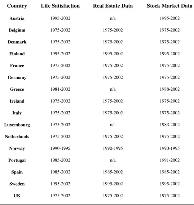
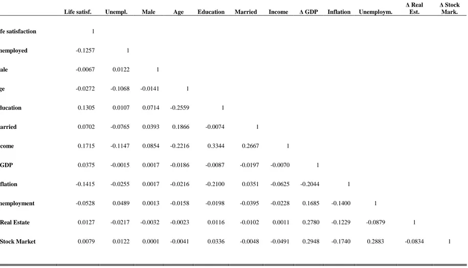
Table 2 provides a detailed description of the availability of data for each country for the three main variables, namely life satisfaction, stock market and real estate prices. Table 3 reports summary statistics. The average real stock price increase is around 2.5 times higher than the real estate one, while the standard deviation is more than three times bigger. Stock markets are characterized by higher risk but provide higher returns to investors. Following Di Tella, MacCulloch and Oswald (2001), the original variable “Income”, which ranged from 1 to 13, has been recoded in order to obtain four dummy variables for four different income groups8. Table 4 shows pairwise correlations to check for possible multicollinearity among the variables of interest. All the correlations are well below 0.509.
Two things deserve to be underlined. First, there is a negative correlation between age and income, which is due to the effect of retirement and to the fact that the education level in European countries has constantly risen over time. The correlation between age and education is negative: young people are more educated than old ones. Since higher qualifications imply higher wages (positive correlation between education and income), it turns out that the correlation between income and age is negative. Second, the correlation between stock market and real estate changes is negative, even if the relation is statistically significant (t-value equal to -78.95) but economically not very strong (coefficient equal to -0.0834).
This negative correlation can be explained by the fact that people disinvest in one market to invest in the booming one. Alternatively, Lustig and Van Nieuwerburgh (2005) elaborate a model with housing collateral where the ratio of housing wealth to human wealth shifts the conditional distribution of asset prices and consumption growth. A decrease in real estate prices reduces the collateral value of housing, increases household exposure to idiosyncratic risk and increases the conditional market price of risk. Using
6 This methodology has been adopted because the database provided by the BIS does not provide total
returns for the real estate market (including rents) and because the target was to focus on simple fluctuations of aggregate price levels rather than on total yields.
7 See, for example, Di Tella, MacCulloch and Oswald (2001), Di Tella and MacCulloch (2003), Alesina, Di
Tella and MacCulloch (2004) and Becchetti, Castriota and Giuntella (2006).
8
Income 1 includes the groups 1-3, Income 2 the groups 4-6, income 3 the groups 7-9 and income 4 the groups 10-13.
9 It would have been interesting to add in the regression the GDP per capita as an additional control
variable. Unfortunately there is a multicollinearity problem between the GDP per capita on one side and inflation and unemployment rates on the other. In fact, the correlation between GDP per capita and inflation is -0.57 and that between GDP per capita and unemployment -0.50. Nevertheless, the effect of the GDP per capita is in big part captured by the country dummy variable.
aggregate data for the United States they find that a decrease in the ratio of housing wealth to human wealth predicts higher returns on stocks.
The econometric methodology adopted in this research is standard in the literature and is based on multinomial ordered probit regressions with heteroskedasticity-robust standard errors. The model specification is:
ijt L l ljt l K k kijt k t j
ijt MICRO MACRO
S =α +λ +
∑
β +∑
γ +ε=
=1 1
where the satisfaction level Sijt of individual i in country j at time t is affected by a country dummy variable αj which captures all the economic, political, social etc. unobserved country-specific components, a year dummy λt, a set of microeconomic characteristics MICROkijt, and a set of macroeconomic variables MACROmjt, while εijt represents the individual idiosyncratic error. The MICROkijt characteristics are the variables from the Eurobarometer listed in the upper part of Table 1, while the MACROmjt are the remaining ones in the lower part.
4. Empirical results
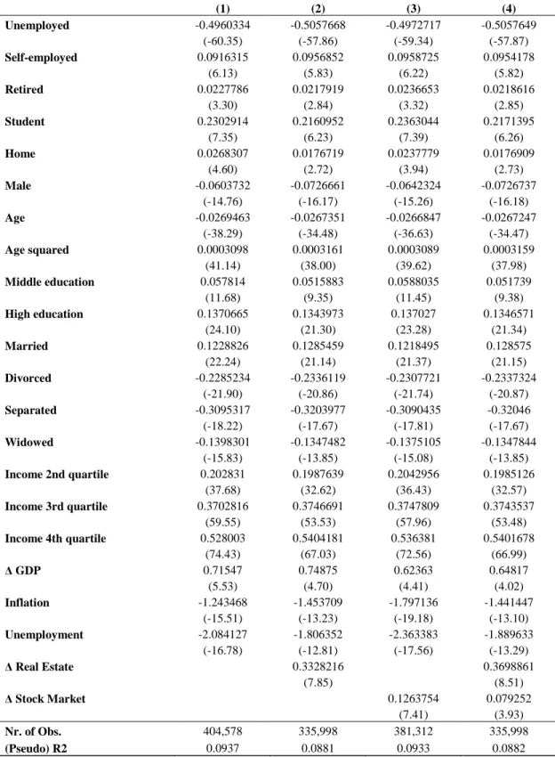
Table 5 presents preliminary results from full sample regressions. Column 1 includes all the variables listed in Table 1, but stock market and real estate variations. It can be considered as a reference equation. In line with previous results, being unemployed has a strong negative effect on well-being, happiness is U-shaped with age while education, income and a stable and successful relationship exert a positive effect. Columns 2 and 3 repeat the same exercise by adding real estate and stock market price variations separately. Column 4 adds the two regressors together. Notice that the number of observations diminishes when including real estate price variations since housing data for Austria, Greece, Luxembourg and Portugal are not available.
Two results emerge from this table. First, increases of both house and stock prices have a positive effect on life-satisfaction. Second, variations in house prices are more important in relative and absolute terms. From Column 4 we can see that the coefficient of ∆ Real Estate is around five times bigger than the coefficient of ∆ Stock Market, therefore in relative terms real estate fluctuations have a bigger impact on peoples’ lives. The effect in absolute terms is still higher for house price fluctuations. In fact, although average stock market returns are higher than real estate ones, since the coefficient of ∆ Real Estate is five times bigger than that of ∆ Stock Market, the final average impact of house price fluctuations is more than twice as big as that of stock price ones. This can be due to the higher share of real estate assets in the household portfolio (most people, especially in Southern Europe, own the house where they live), to the psychological reason that real estate prices are perceived to be more permanent or to the fact that houses can be used as collateral to relax borrowing constraints and obtain loans from a financial institution.
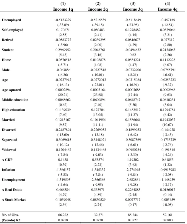
The third main result of this paper emerges from Tables 6 and 7 which report robustness checks with regressions by age and income subgroups. It would have been reasonable to expect different coefficient values for the two financial variables in different income groups and age cohorts, since young and poor people likely rent the place they live in and do not own stocks, while richer and older people have more financial assets and real estate properties. If on average this were the case we should observe positive coefficients for high-income and older people, since they would experience an increase in their permanent income and would weaken their borrowing constraints (if need be). On the contrary, we should observe a negative coefficient for ∆ Real Estate in the low-income and young-people groups since they are less likely to own their house, thus the effect of higher rents and mortgages would prevail. The coefficient of ∆ Stock Market for low-income and young people might be slightly positive, driven by the positive effect of the few individuals who own assets, or null, in case social comparison generates frustration among poor people and counterbalances the positive effect.
If these arguments were true there would be important policy implications since there would be social conflicts among age cohorts and income groups. This would be true especially for the real estate market where gains and losses due to house price fluctuations would be perceived as a zero-sum game: the capital gain of the old/rich is paid by the young/poor through higher rents and mortgages. In order to avoid social conflicts, policymakers interested in the value of economic fairness should consider every measure aimed at discouraging real estate as a form of speculative investment like, for example, higher taxes on second and third houses, very high capital gain taxes for properties sold before a certain number of years from the time of purchase etc.
Surprisingly enough, results from Tables 6 and 7 do not support these arguments. The coefficients of both ∆ Real Estate and ∆ Stock Market are always non-negative in all sub-groups, while a negative coefficient would have been expected for low-income and young-age individuals at least for ∆ Real Estate. Furthermore, older age-cohorts and higher income groups do not have higher coefficients for both variables than the rest of the sample. On the contrary, the coefficients of both stock and house price increases seem to be statistically not significant in higher income groups.
There are three possible explanations for this unexpected result. First, people with a lower income are more in need (higher ratio between change of wealth and personal income). Richer people are less sensitive to price changes because, excluding big speculators, their quality of life will hardly be compromised by market fluctuations, whereas for poor people a gain can be small in absolute terms but high in relative ones. Second, the borrowing constraints of poor people are more heavily affected by the house prices, provided that one has an asset to give as collateral. Third, the process through which expectations about future price changes are generated might differ across income and age cohorts. More specifically, while young and poor people might believe that house prices will continue along the previous path, the others might be more aware of the future likely market evolutions. Young and poor people might be affected by the illusion that prices will be rising or falling forever, while high income people (who on average
have a higher education level) and old people (who have accumulated experience over time) might be aware of the fact that, sooner or later, after a boom there is always a bust.
5. Conclusions
This paper studies the welfare effects of real estate and stock market fluctuations using data from the Eurobarometer on the self-declared life-satisfaction levels of 400,000 Western European citizens from 1975 to 2002. Three main conclusions emerge. First, both housing and stock price increases have a positive impact on human well-being. Second, real estate fluctuations are more important than stock market ones, both in relative and absolute terms, which is in line with previous research about the effects of these two sources of wealth on consumption. Third, when performing a sensitivity analysis with regressions by age and income subgroups it emerges that old and high income people do not have higher welfare gains than young and poor ones. This latter result is particularly important for the real estate market. In fact, it would seem natural to believe that a welfare maximizing policy should keep down house prices in order to allow everybody, especially in low-income and young age cohorts, to enter the housing market or to pay low rents. Unfortunately, the empirical results in this paper show that the positive effects of rising house prices counterbalance the negative effects. This might be due to the fact that rising house prices allow households to relax their borrowing constraints in case they decide to use a real estate property as collateral. Since young and poor people are more in need, this might explain the higher sensitivity of these groups to the real estate fluctuations.
Legend: DV = Dummy Variable.
Table 1: Description of the variables used
Name Source Variable
Life satisfaction Eurobarometer Self-declared life-satisfaction level from 1 (not at all satisfied) to 4 (very satisfied)
Full employed Eurobarometer DV which takes value 1 if the respondent is full employed, 0 otherwise
Unemployed Eurobarometer DV which takes value 1 if the respondent is unemployed, 0 otherwise
Self-employed Eurobarometer DV which takes value 1 if the respondent is self-employed, 0 otherwise
Retired Eurobarometer DV which takes value 1 if the respondent is retired, 0 otherwise
Student Eurobarometer DV which takes value 1 if the respondent is student, 0 otherwise
Home Eurobarometer DV which takes value 1 if the respondent is responsible for home and not working, 0 otherwise
Male Eurobarometer DV which takes value 1 if the respondent is male, 0 otherwise
Age Eurobarometer Age of the respondent in years
Age squared Eurobarometer Square of the respondent's age in years
Low education Eurobarometer DV which takes value 1 if the respondent has less than 15 years of education, 0 otherwise
Middle education Eurobarometer DV which takes value 1 if the respondent has 15-18 years of education, 0 otherwise
High education Eurobarometer DV which takes value 1 if the respondent has more than 18 years of education, 0 otherwise
Single Eurobarometer DV which takes value 1 if the respondent is single, 0 otherwise
Married Eurobarometer DV which takes value 1 if the respondent is married, 0 otherwise
Divorced Eurobarometer DV which takes value 1 if the respondent is divorced, 0 otherwise
Separated Eurobarometer DV which takes value 1 if the respondent is separated, 0 otherwise
Widowed Eurobarometer DV which takes value 1 if the respondent is widowed, 0 otherwise
Income 1 Eurobarometer DV which takes value 1 if the respondent belongs to the lowest income group, 0 otherwise
Income 2 Eurobarometer DV which takes value 1 if the respondent belongs to the 2nd income group, 0 otherwise
Income 3 Eurobarometer DV which takes value 1 if the respondent belongs to the 3rd income group, 0 otherwise
Income 4 Eurobarometer DV which takes value 1 if the respondent belongs to the highest income group, 0 otherwise
∆ GDP World Bank Growth rate of the GDP per capita in 2000 constant US $, three-year moving average
Inflation World Bank Inflation rate, three-year moving average
Unemployment OECD Unemployment rate, three-year moving average
∆ Real Estate BIS Growth rate of real house prices (net of inflation), three-year moving average
∆ Stock Market Ecowin/Datastream Growth rate of real stock market prices (net of inflation), three-year moving average
Table 2: Availability of Data on Life Satisfaction and Asset Prices
Country Life Satisfaction Real Estate Data Stock Market Data
Austria 1995-2002 n/a 1995-2002 Belgium 1975-2002 1975-2002 1975-2002 Denmark 1975-2002 1975-2002 1975-2002 Finland 1995-2002 1995-2002 1995-2002 France 1975-2002 1975-2002 1975-2002 Germany 1975-2002 1975-2002 1975-2002 Greece 1981-2002 n/a 1988-2002 Ireland 1975-2002 1975-2002 1975-2002 Italy 1975-2002 1975-2002 1975-2002 Luxembourg 1975-2002 n/a 1983-2002 Netherlands 1975-2002 1975-2002 1975-2002 Norway 1990-1995 1990-1995 1990-1995 Portugal 1985-2002 n/a 1991-2002 Spain 1985-2002 1985-2002 1985-2002 Sweden 1995-2002 1995-2002 1995-2002 UK 1975-2002 1975-2002 1975-2002
Table 4: Pairwise Correlation Matrix
Life satisf. Unempl. Male Age Education Married Income ∆ GDP Inflation Unemploym.
∆ Real Est. ∆ Stock Mark. Life satisfaction 1 Unemployed -0.1257 1 Male -0.0067 0.0122 1 Age -0.0272 -0.1068 -0.0141 1 Education 0.1305 0.0107 0.0714 -0.2559 1 Married 0.0702 -0.0765 0.0393 0.1866 -0.0074 1 Income 0.1715 -0.1147 0.0854 -0.2216 0.3344 0.2667 1 ∆ GDP 0.0375 -0.0015 0.0017 -0.0186 -0.0087 -0.0197 -0.0070 1 Inflation -0.1415 -0.0255 0.0017 -0.0216 -0.2100 0.0351 -0.0625 -0.2044 1 Unemployment -0.0528 0.0489 0.0013 -0.0158 -0.0198 -0.0395 -0.0228 0.1685 -0.1400 1 ∆ Real Estate 0.0127 -0.0217 -0.0032 -0.0023 0.0116 -0.0102 0.0011 0.2780 -0.1229 -0.0879 1 ∆ Stock Market 0.0079 0.0122 0.0001 -0.0041 0.0336 -0.0048 -0.0491 0.2948 -0.1740 0.2883 -0.0834 1
Table 5: Life-Satisfaction Equations, Full Sample
(1) (2) (3) (4) Unemployed -0.4960334 -0.5057668 -0.4972717 -0.5057649 (-60.35) (-57.86) (-59.34) (-57.87) Self-employed 0.0916315 0.0956852 0.0958725 0.0954178 (6.13) (5.83) (6.22) (5.82) Retired 0.0227786 0.0217919 0.0236653 0.0218616 (3.30) (2.84) (3.32) (2.85) Student 0.2302914 0.2160952 0.2363044 0.2171395 (7.35) (6.23) (7.39) (6.26) Home 0.0268307 0.0176719 0.0237779 0.0176909 (4.60) (2.72) (3.94) (2.73) Male -0.0603732 -0.0726661 -0.0642324 -0.0726737 (-14.76) (-16.17) (-15.26) (-16.18) Age -0.0269463 -0.0267351 -0.0266847 -0.0267247 (-38.29) (-34.48) (-36.63) (-34.47) Age squared 0.0003098 0.0003161 0.0003089 0.0003159 (41.14) (38.00) (39.62) (37.98) Middle education 0.057814 0.0515883 0.0588035 0.051739 (11.68) (9.35) (11.45) (9.38) High education 0.1370665 0.1343973 0.137027 0.1346571 (24.10) (21.30) (23.28) (21.34) Married 0.1228826 0.1285459 0.1218495 0.128575 (22.24) (21.14) (21.37) (21.15) Divorced -0.2285234 -0.2336119 -0.2307721 -0.2337324 (-21.90) (-20.86) (-21.74) (-20.87) Separated -0.3095317 -0.3203977 -0.3090435 -0.32046 (-18.22) (-17.67) (-17.81) (-17.67) Widowed -0.1398301 -0.1347482 -0.1375105 -0.1347844 (-15.83) (-13.85) (-15.08) (-13.85) Income 2nd quartile 0.202831 0.1987639 0.2042956 0.1985126 (37.68) (32.62) (36.43) (32.57) Income 3rd quartile 0.3702816 0.3746691 0.3747809 0.3743537 (59.55) (53.53) (57.96) (53.48) Income 4th quartile 0.528003 0.5404181 0.536381 0.5401678 (74.43) (67.03) (72.56) (66.99) ∆ GDP 0.71547 0.74875 0.62363 0.64817 (5.53) (4.70) (4.41) (4.02) Inflation -1.243468 -1.453709 -1.797136 -1.441447 (-15.51) (-13.23) (-19.18) (-13.10) Unemployment -2.084127 -1.806352 -2.363383 -1.889633 (-16.78) (-12.81) (-17.56) (-13.29) ∆ Real Estate 0.3328216 0.3698861 (7.85) (8.51) ∆ Stock Market 0.1263754 0.079252 (7.41) (3.93) Nr. of Obs. 404,578 335,998 381,312 335,998 (Pseudo) R2 0.0937 0.0881 0.0933 0.0882Legend: results are from ordered probit models with heteroskedasticity-robust standard errors. Full-employed, female, low-education, single, income 1, 1975 and France are the base to avoid perfect multicollinearity.
Table 6: Life-Satisfaction Equations, by Age Sub-Groups
(1) (2) (3) (4) <29 29-41 42-64 >64 Unemployed -0.5036549 -0.544279 -0.5144035 -0.2660041 (-33.35) (-32.01) (-33.81) (-4.92) Self-employed 0.1245006 0.1342063 0.0544548 0.1805011 (2.88) (4.98) (2.14) (2.36) Retired -0.1562618 -0.3670247 -0.0248953 0.0232976 (-1.96) (-8.31) (-2.16) (1.30) Student 0.171725 0.0466115 -0.1646662 0.2763582 (4.16) (0.45) (-0.71) (0.67) Home -0.0421836 0.031101 0.0232598 0.0348306 (-2.64) (2.64) (2.19) (1.61) Male -0.1019545 -0.0957266 -0.067148 -0.0011111 (-10.31) (-11.20) (-8.62) (-0.10) Age -0.0309728 -0.0504129 -0.1027401 0.0501019 (-1.61) (-2.34) (-10.40) (3.20) Age squared 0.0003498 0.0006046 0.0010893 -0.0002807 (0.84) (1.96) (11.44) (-2.65) Middle education 0.004439 0.0992982 0.0635202 0.0407673 (0.25) (7.83) (7.48) (3.71) High education 0.0997191 0.1639343 0.1104862 0.1552002 (5.23) (12.12) (10.77) (10.50) Married 0.1550004 0.1874174 0.0680134 0.0538742 (14.08) (15.90) (5.28) (2.80) Divorced -0.3302941 -0.1984472 -0.2442561 -0.2517314 (-7.97) (-9.46) (-13.68) (-7.73) Separated -0.2823545 -0.2831956 -0.364707 -0.311944 (-5.55) (-9.38) (-12.30) (-5.16) Widowed -0.0089785 -0.1011369 -0.1800681 -0.1640562 (-0.09) (-2.22) (-10.04) (-8.41) Income 2nd quartile 0.1994848 0.2090695 0.2265962 0.1505246 (14.01) (13.87) (21.03) (13.75) Income 3rd quartile 0.3567667 0.3992716 0.4182317 0.3572327 (22.76) (24.85) (34.29) (21.91) Income 4th quartile 0.4955649 0.5811161 0.6142364 0.4592749 (27.48) (33.06) (44.36) (19.64) ∆ GDP 0.73704 1.06228 0.27815 0.68367 (2.05) (3.39) (1.02) (1.81) Inflation -1.450975 -1.709234 -1.407714 -0.9406322 (-5.73) (-8.01) (-7.65) (-3.61) Unemployment -1.538865 -1.941503 -2.40251 -1.279933 (-4.46) (-7.14) (-10.04) (-3.96) ∆ Real Estate 0.3777115 0.5716349 0.2945589 0.2667923 (3.82) (6.87) (3.97) (2.65) ∆ Stock Market 0.0652343 0.1343323 0.0326867 0.0933301 (1.39) (3.44) (0.98) (1.97) Nr. of Obs. 62,065 92,995 118,130 62,808 (Pseudo) R2 0.0900 0.1017 0.0911 0.0721Legend: results are from ordered probit models with heteroskedasticity-robust standard errors. Full-employed, female, low-education, single, income 1, 1975 and France are the base to avoid perfect multicollinearity.
Table 7: Life-Satisfaction Equations, by Income Sub-Groups
(1) (2) (3) (4)
Income 1q Income 2q Income 3q Income 4q
Unemployed -0.5123229 -0.5215539 -0.5118649 -0.457155 (-33.09) (-39.18) (-23.95) (-12.54) Self-employed 0.170671 0.080483 0.1278482 0.0879066 (2.55) (2.41) (4.15) (3.21) Retired -0.0583772 0.0239295 0.0816673 0.077312 (-3.96) (2.00) (4.29) (2.80) Student 0.2969952 0.2048761 -0.0494632 0.2134063 (5.43) (3.16) 0.62 (2.26) Home -0.0876518 0.0108878 0.0584221 0.1112228 (-5.71) (1.08) (4.47) (6.07) Male -0.063886 -0.0727818 -0.0732906 -0.0755791 (-6.26) (-10.01) (-8.21) (-6.61) Age -0.0237942 -0.0272012 -0.0315084 -0.0253223 (-16.13) (-22.01) (-16.94) (-9.37) Age squared 0.0002894 0.0003164 0.0003688 0.0002968 (20.21) (23.68) (17.44) (9.63) Middle education 0.0068662 0.0600894 0.0648747 0.0610231 (0.62) (7.40) (5.30) (3.04) High education 0.1139039 0.127704 0.1482512 0.1294784 (7.60) (13.05) (11.27) (6.42) Married 0.1213167 0.1041956 0.1586664 0.1943037 (9.52) (11.11) (11.94) (10.67) Divorced -0.2487894 -0.2269953 -0.1899953 -0.144928 (-13.60) (-13.18) (-6.42) (-3.43) Separated -0.3069615 -0.3448921 -0.3087569 -0.1733739 (-10.12) (-12.46) (-6.61) (-2.76) Widowed -0.1204462 -0.1434465 -0.0950754 -0.191515 (-7.84) (-9.03) (-3.30) (-4.24) ∆ GDP 0.1438 0.55574 1.19302 0.61853 (0.39) (2.22) (3.62) (1.32) Inflation -1.566157 -1.345332 -2.274945 -0.9915983 (-5.83) (-7.84) (-9.84) (-3.08) Unemployment -1.519593 -2.366366 -2.682861 -1.148939 (-4.64) (-9.95) (-9.28) (-3.17) ∆ Real Estate 0.466384 0.333971 0.2264883 0.0186017 (4.79) (4.89) (2.45) (0.14) ∆ Stock Market 0.1059048 0.0830529 0.0077717 -0.005459 (2.56) (2.74) (0.17) (-0.08) Nr. of Obs. 66,222 132,371 85,244 52,161 (Pseudo) R2 0.0738 0.0770 0.0827 0.0800
Legend: results are from ordered probit models with heteroskedasticity-robust standard errors. Full-employed, female, low-education, single, 1975 and France are the base to avoid perfect multicollinearity.
References
[1] Alesina, A., Di Tella, R. and MacCulloch, R. (2004). “Happiness and Inequality: Are Europeans and Americans different?”. Journal of Public Economics, Vol. 88, pp. 2009-2042.
[2] Ando, A. and Modigliani, F. (1963), “The ‘Life Cycle’ Hypothesis of Saving: Aggregate Implications and Tests”, American Economic Review, No. 53.
[3] Bhatia
[4] Bayoumi, T. (1993), “Financial Deregulation and Household Saving”, Economic Journal, Vol. 103.
[5] Becchetti, L., Castriota, S. and Giuntella, O. (2006), “The Effects of Age and Job
Protection on the Welfare Costs of Inflation and Unemployment: a Source of ECB anti-inflation bias?”, CEIS Working Paper, No. 245, available on line at the address
www.ceistorvergata.it .
[6] Benjamin, J.D., Chinloy, P. and Jud, G.D. (2004), “Real Estate Versus Financial
Wealth in Consumption”, Journal of Real Estate Finance and Economics, No. 29:3.
[7] Berg, L. and Bergström, R. (1995), Housing and Financial Wealth, Financial
Deregulation, and Consumption-The Swedish Case”, Scandinavian Journal of Economics, No. 97.
[8] Bhatia, K. (1987), “Real Estate Assets and Consumer Spending”, Quarterly Journal of
Eocnomics, Vol. 102.
[9] Blanchflower, D. G. and Oswald, A. J. (2004), “Well-Being over time in Britain and
the USA”, Journal of Public Economics, Vol. 88.
[10] Boone, L. and Girouard, N. (2002), “The Stock Market, the Housing Market and
Consumer Behavior”, OECD Working Paper, No. 35, available on line at the address
www.oecd.org .
[11] Bostic, R., Gabriel, S. and Painter, G. (2005), “Housing Wealth, Financial Wealth, and
Consumption: New Evidence from Micro Data”, Working Paper, University of Southern California.
[12] Brodin, P.A. and Nymoen, R. (1992), “Wealth Effects and Exogeneity: the Norwegian Consumption Function 1966(1)-1989(4)”, Oxford Bulletin of Economics and Statistics, Vol. 54(3).
[13] Campbell, J. and Cocco, J. (2005), “How do House Prices Affect Consumption? Evidence from Micro Data”, forthcoming in the Journal of Monetary Economics. [14] Case, K.E. (1992), “The Real Estate Cycle and the Economy: Consequences of the
Massachussets Boom of 1984-1987”, Vol. 29.
[15] Case, K.E., Quigley, J.M. and Shiller, R.J. (2005), “Comparing Wealth Effects: the
Stock Market Versus the Housing Market”, Advances in Macroeconomics, Vol. 5(1).
[16] Castriota, S. (2006), “Education and Happiness: a Further Explanation to the Easterlin
Paradox?”, CEIS Working Paper No. 246, available on line at the address
www.ceistorvergata.it .
[17] Castriota, S. and Van Hoorn, A. (2007), “The Impact of Economic Variables on
Human Well-Being”, Mimeo.
[18] Diener, E. and Oishi, S. (2000), “Money and Happiness: Income and Subjective
Well-Being Across Nations”, in “Culture and Subjective Well-Well-Being”, Cambridge, MIT Press.
[19] Di Tella, R. and MacCulloch, R. (2003). “The Macroeconomics of Happiness”, Review of Economics and Statistics. November 2003, 85(4): 809–827, MIT Press.
[20] Di Tella, R., MacCulloch, R. J. and Oswald, A. J. (2001), “Preferences over Inflation
and Unemployment: Evidence from Surveys of Happiness”, American Economic Review, Vol. 91, No. 1.
[21] Dvornak, N. and Kohler, M. (2003), “Housing Wealth, Stock Market Wealth and
Consumption: a Panel Analysis for Australia”, Research Discussion Paper, No. 203-07, Reserve Bank of Australia.
[22] Easterlin, R. (1974), “Does Economic Growth Improve the Human a lot? Some
Empirical Evidence”, in Nations and Households in Economic Growth: Essays in Honor of Moses Abramowitz. New York and London, Academic Press.
[23] Elliott, J.W. (1980), “Wealth and Wealth Proxies in a Permanent Income Model”,
Quarterly Journal of Economics, Vol. 95.
[24] Engelhardt, G.V. (1994), “House Prices and the Decision to Save for Down Payments”,
New England Economic Review, May-June 1994: 47-58.
[25] Engelhardt, G.V. (1996), “House Prices and Home Owner Saving Behavior”, Regional
Science and Urban Economics, Vol. 26.
[26] Englund, P. and Ioannides, Y.M. (1997), “House Price Dynamics: an International
Empirical Perspective”, Journal of Housing Economics, Vol. 6.
[27] Frey B. S. and Stutzer, A. (2002), “Happiness & Economics”, Princeton University
Press.
[28] Fiedman, M. (1957), “A Theory of the Consumption Function”, Princeton University
Press, Princeton.
[29] Fiedman, B. (2006), “The Moral Consequences of Economic Growth”, Vintage Press.
[30] Koskela, E., Loikkanen, H. and Viren, M. (1992), “House Prices, Household Saving
and Financial Market Liberalization in Finland”, European Economic Review, Vo. 36.
[31] Lettau, M. and Ludvigson, S.C. (2004), “Understanding Trend and Cycle in Asset
Values: Reevaluating the Wealth Effect on Consumption”, American Economic Review, No. 94(1).
[32] Levin, L. (1998), “Are Assets Fungible? Testing the Behavioral Theory of Life-Cycle
Savings”, Journal of Economic Organization and Behavior, Vol. 36.
[33] Lustig, H.N. and Van Nieuwerburgh (2005), “Housing Collateral, Consumption
Insurance, and Risk Premia: an Empirical Perspective”, The Journal of Finance, Vol. LX, No. 3.
[34] Layard, R. (2006), “Happiness, Lessons from a New Science”, Penguin Press.
[35] Lehnert, A. (2004), “Housing, Consumption, and credit Constraints”, Working Paper
No. 2004-63, Federal Reserve Board, Washington, D.C,.
[36] Malthus, T. S. (1798), “An Essay on the Principle of Population”, Cambridge Texts in in
the History of Political Thought, Cambridge University Press, 1992.
[37] Norman, B., Barriel, M. and Weeken, O. (2002), “Equity Wealth and
Consumption-The Experience of Germany, France and Italy in an International Context”, Bank of England Quarterly Bulletin, Spring 2002.
[38] Oswald, A. J. (1997), “Happiness and Economic Performance”, Economic Journal, Vol.
107, No. 445.
[39] Skinner, J. (1989), “Housing Wealth and Aggregate Saving”, Regional Science and
Urban Economics, Vol. 19.
[40] Veenhoven, R. (1993), “Happiness in Nations: Subjective Application of Life in 56
Nations”, Rotterdam: Erasmus University.
[41] Yashikawa, H. and Ohtake, F. (1989), “Female Labor Supply, Housing Demand, and