Closed and open set
classification of real and AI
synthesised speech
by: Michelangelo Medori matr.: 878025 Supervisor: Fabio Antonacci Co-supervisors: Paolo Bestagini Clara Borrelli Academic Year 2019-2020Huge advancements in the development of artificial intelligence tech-niques have been made in the last decade, which have led to the diffusion and spread of computer generated multimedia content, consisting of im-ages, audio and video, which is so realistic that it makes it difficult to be told apart from original content of the same nature.
While there are interesting applications to artificial intelligence gen-erated content, it can also be used in dangerous and deceiving ways, for example as proof in a court of law. Hence it is more and more urgent to find automatic ways to distinguish artificial intelligence synthesised content from original content.
In this paper we take into account audio content, and in particular speech, which is obviously utterly delicate as it comes to forgery. We are going to deepen the previous research made in the field of bispectral analysis in order to create more general automatic methods to recognise real speakers from artificial intelligence synthesised speech.
The dataset of voices that we have used is very wide and heteroge-neous, consisting of both real voices and voices synthesised using various different methods. We extracted the Bicoherence from all the speech recordings and performed some classifications (both multilabel classifi-cations, which consist in distinguishing each class of voices from all the others, and binary classifications between real and fake voices) using vari-ous machine learning techniques, such as support vector machine, logistic regression and random forest.
In particular, once the bicoherences have been computed from the audio files, we performed the following tests. First of all we replicated the tests made on previous works extracting from the bicoherences a set of features which consist on mean, variance, skewness and kurtosis of both the modules and the phases of the bicoherences and trying to clas-sify them performing simple multiclass and binary classifications using a support vector machine, a series of logistic regressors and a random forest.
Then we simulated an open set environment using a series of support vector machines, in order to test the model with data not yet seen in the training phase.
Moreover, we used a series of U-Nets to extract a new set of features and tried to classify them performing simple multi-label and binary clas-sifications.
Finally, we concatenated the two set of features above and performed more classifications with them (in this case also with an open set envi-ronment) and we are going to show that with this method we obtained the best results.
We hope that these results can clarify better the role of bispectral analysis in distinguishing between real and fake speech recordings, and could lead to more research in the field of multimedia forensics.
Nell’ultimo decennio sono stati fatti grandi passi avanti nello sviluppo di tecniche di intelligenza artificiale, che hanno permesso la diffusione in larga scala di contenuti multimediali generati artificialmente, come audio, immagini e video che sono talmente realistici da risultare praticamente impossibili da distinguere da contenuti multimediali originali dello stesso tipo. Nonostante ci siano molte interessanti applicazioni per questo ma-teriale generato algoritmicamente, questo può essere usato anche in modo improprio e pericoloso, per esempio come prova in una corte di giustizia. Per questo motivo, risulta sempre più urgente trovare modi auto-matici per distinguere contenuti multimediali generati da intelligenze ar-tificiali da quelli originali.
In questa tesi prendiamo in considerazione contenuti audio, e ci oc-cuperemo in particolare del parlato, che è ovviamente molto delicato nel momento in cui venga “falsificato”. Andremo ad ampliare la ricerca fatta in lavori precedenti riguardo l’analisi bispettrale al fine di creare metodi automatici il più possibile generali per distinguere il parlato sintetico da quello registrato da parlatori veri.
Il dataset che abbiamo usato è molto ampio ed eterogeneo, e consiste sia di voci “vere” che di voci generate algoritmicamente con vari metodi di sintetizzazione. Abbiamo estratto le bicoerenze da tutte le registrazioni di parlato, e abbiamo provato fare delle classificazioni (sia classificazioni multi-label, che consistono nel distinguere ogni classe da tutte le altri, sia classificazioni binarie, per distinguere le voci vere da quelle finte) usando vari metodi di machine learning come support vector machine, logistic regression e random forest.
In particolare, una volta calcolate le bicoerenze, abbiamo eseguito i seguenti test: per prima cosa abbiamo replicato gli esperimenti fatti in lavori precedenti estraendo dei descrittori (che consistono nei primi quattro momenti statistici) sia dai moduli che dalle fasi delle bicoerenze e provando a classificarli per mezzo di semplici classificazioni (sia multi-label che binarie) usando una support vector machine, una serie di logistic regression e una Random forest; a seguire abbiamo simulato un ambiente open set usando una serie di support vector machine, al fine di testare il modello con dati mai visti nella fase di training; inoltre abbiamo us-ato delle reti neurali chiamate U-Net per estrarre un nuovo insieme di descrittori che abbiamo provato a classificare tramite semplici classifi-cazioni multi-label e binarie; infine abbiamo concatenato i due insiemi di
descrittori di cui sopra e abbiamo provato a classificarli, sta volta simu-lando anche un ambiente open set, e mostreremo che in questo modo si ottengono i risultati migliori.
Ci auguriamo che il lavoro fatto possa chiarire meglio il ruolo che ha l’analisi bispettrale nel distinguere il parlato vero da quello sintetizzato da intelligenza artificiale, e possa aprire la strada ad altra ricerca nell’ambito dell’audio forense.
Ogni cosa ha un inizio e una fine.
In questo caso la fine (ovvero i ringraziamenti) coincide con l’inizio (di questa tesi).
Inizierei subito col ringraziare Clara, Fabio e Paolo, che sono stati fon-damentali per il compimento di questo lavoro, e dai quali ho imparato molto nel corso del mio ultimo anno di studi universitari.
Un altro importante ringraziamento va ai miei colleghi (i "Cremonesi"), ovvero Edo, Jackie, Malvo, Marzo, Molgo e Vago: senza di voi non sarei arrivato a questo punto.
Una menzione speciale va a Marta e Robin, che mi hanno sostenuto negli ultimi mesi, aiutandomi a superare delle difficoltà impossibili da trascu-rare.
Un ulteriore importante ringraziamento va alla mia famiglia, e in parti-colare a mia madre, che ha vissuto in prima persona il superamento di ogni ostacolo che ho dovuto affrontare lungo questo cammino.
Infine, a tutti coloro che non sono stati menzionati, va un ringraziamento per i bei momenti passati insieme...e anche per quelli brutti: dopotutto l’importante è riuscire ad andare avanti senza farsi abbattere.
Questo lavoro è dedicato a tutti coloro che sanno ascoltare. Che la fine di questo capitolo sia l’inizio di uno migliore. Nella foto sotto, il co-autore di questa tesi.
In memoria di Alessio Nava 1994-2018
Abstract i
Sommario iii
Ringraziamenti v
List of Figures xiii
List of Tables xv
Glossary xvi
Introduction xix
1 Theoretical Background 1
1.1 Features extraction, features normalisation and
dimension-ality reduction . . . 1
1.1.1 Features extraction and normalisation . . . 2
1.1.2 Dimensionality reduction techniques . . . 3
1.2 Machine learning techniques and classification algorithms 7 1.2.1 Classification problems . . . 9
1.2.2 Support vector machine . . . 10
1.2.3 Logistic regression . . . 11
1.2.4 Decision tree and Random Forest . . . 12
1.2.5 Convolutional neural networks . . . 13
1.2.6 Convolutional autoencoder and U-Net . . . 15
1.2.7 Closed set vs open set classification . . . 16
1.3 Confusion matrix, accuracy and ROC curve . . . 17
1.3.1 Confusion matrix . . . 17
1.3.2 Accuracy and other metrics . . . 18
1.3.3 ROC curve . . . 19
2 State of the Art 20 2.1 Overview on Multimedia Forensics . . . 20
2.2 Speech Synthesis: text to speech and voice conversion al-gorithms . . . 23
2.2.1 Text to speech synthesis . . . 23
2.2.2 Voice conversion synthesis . . . 26 vii
2.3 Recognising real speakers from AI synthesised speech . . 27
2.3.1 Methods based on classical feature extraction . . 28
2.3.2 Methods based on data driven features . . . 32
3 Problem formulation and proposed methodologies 34 3.1 Problem formulation . . . 34
3.2 Proposed Methodologies . . . 35
3.2.1 Feature extraction . . . 36
3.2.2 Feature normalisation and dimensionality reduction 43 3.2.3 Closed set classification . . . 44
3.2.4 Open set classification . . . 45
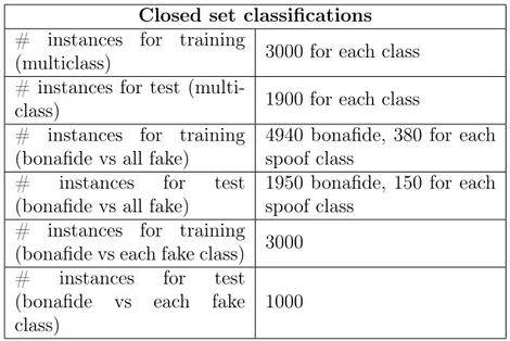
4 Experimental results 50 4.1 Dataset and setup . . . 50
4.2 Closed set classification results . . . 53
4.2.1 Closed set classification of MK features . . . 54
4.2.2 Closed set classification of UNET features . . . . 57
4.2.3 Closed set classification of MKU features . . . 59
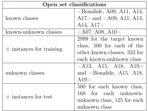
4.3 Open set classification results . . . 61
4.3.1 Open set classification of MK features . . . 62
4.3.2 Open set classification of MKU features . . . 66
5 Conclusions and Future Works 73 Appendices 76 A Results of the classification of the Bicoherences using a convolutional neural network . . . 76
B Results of the classification using a U-Net trained on bonafide bicoherences . . . 78
C Confusion matrixes of all the closed set classification of MK, UNET and MKU features . . . 83
C.1 Confusion matrixes of the closed set classifications of MK features . . . 83
C.2 Confusion matrices of the closed set classifications of UNET features . . . 88
C.3 Confusion matrices of the closed set classifications of MKU features . . . 90
1.1 Example structure of a convolutional neural network used for classification. Taken from https://towardsdatascience.com/a- comprehensive-guide-to-convolutional-neural-networks-the-eli5-way-3bd2b1164a53. . . 15 1.2 Autoencoder structure. . . 16 1.3 Confusion matrix for a two-class classification problem . 18 2.1 General architecture of a text to speech synthesiser. . . . 24 2.2 Modules and phases of the bicoherences extracted from
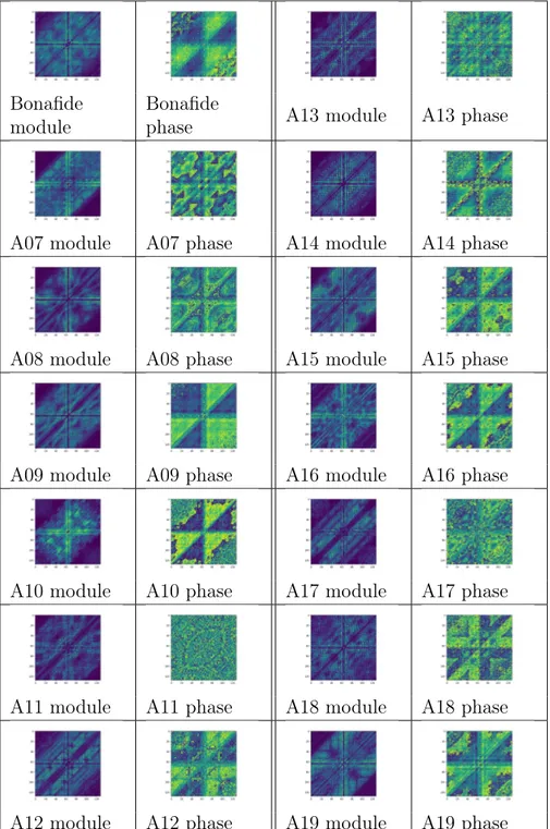
both bonafide speech and speech synthesised with state of the art methods. The picture is taken from [1] . . . 30 3.1 Scheme that shows the three different types of
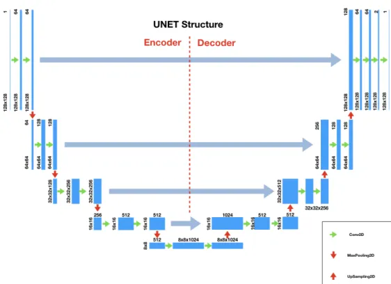
classifica-tion corresponding to the three objectives of this thesis. . 35 3.2 Block diagram of the proposed methodology. . . 36 3.3 Scheme that shows the architecture of the U-Net used for
feature extraction. . . 40 3.4 Feature extraction performed using an autoencoder. . . . 42 3.5 Scheme of the open set classification algorithm which
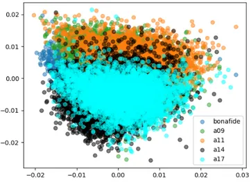
in-volves known-unknown features. . . 47 4.1 2D catter plot of the MK features belonging to the classes
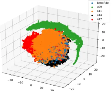
Bonafide, A09, A11, A14 and A17, reduced using t-SNE. 57 4.2 3D scatter plot of the MK features belonging to the classes
Bonafide, A09, A11, A14 and A17 reduced using t-SNE. . 57 4.3 Confusion matrix of a multiclass classification (CSM) that
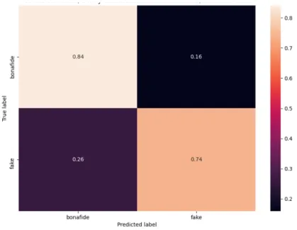
involves MK features, performed using a series of one-versus-the-rest support vector machines. . . 58 4.4 Confusion matrix of a binary (bonafide vs all spoof)
(CS-BVAS) classification that involves MK features, performed using a random forest. . . 58 4.5 Confusion matrix of a multiclass classification (CSM) that
involves UNET features, performed using a series of one-versus-the-rest support vector machines. . . 59 4.6 Confusion matrix of a binary (bonafide vs all spoof)
(CS-BVAS) classification that involves UNET features, per-formed using a logistic regression. . . 59
4.7 2D scatter plot of the MKU features belonging to the classes bonafide, A09, A11, A14 and A17, reduced using PCA. . . 60 4.8 3D scatter plot of the MKU features belonging to the
classes bonafide, A09, A11, A14 and A17, reduced using PCA. . . 60 4.9 2D scatter plot of the MKU features belonging to the
classes bonafide, A09, A11, A14 and A17, reduced using ICA. . . 61 4.10 3D scatter plot of the MKU features belonging to the
classes bonafide, A09, A11, A14 and A17, reduced using ICA. . . 61 4.11 Confusion matrix of a multiclass classification (CSM) that
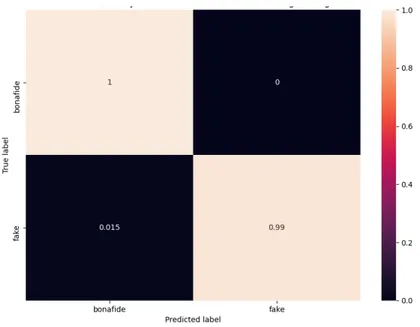
involves MKU features, performed using a series of one-versus-the-rest support vector machines. . . 62 4.12 Confusion matrix of a binary (bonafide vs all spoof)
(CSB-VAS) classification that involves MKU features, performed using a support vector machine. . . 62 4.13 Confusion matrix of an open set classification that involves
the MK features, without known-unknown features, per-formed using bonafide features as known (OSBT1). . . . 63 4.14 Confusion matrix of an open set classification that
in-volves the MK features, with known-unknown features, performed using bonafide features as known (OSBT2). . 63 4.15 Confusion matrix of an open set classification that
in-volves the MK features, with known-unknown features, performed using bonafide features as known (OSBT3). . 64 4.16 Comparison between the three methods for
distinguish-ing known and unknown features that consist in the ROC curves derived by the third version of the open set classi-fier using the scores of the SVMs and the confusion ma-trix of the third classifier, for MK features with bonafide as known. The blue curve corresponds to the maximum scores, while the orange one is associated to the ratio of the scores of the SVMs. The red dot represents the con-fusion matrix related to the third version of the open set classification algorithm (OSBT3). . . 65 4.17 Confusion matrix of an open set classification that involves
the MK features, without known-unknown features, per-formed using bonafide features as unknown (OSST1). . 66 4.18 Confusion matrix of an open set classification that
in-volves the MK features, with known-unknown features, performed using bonafide features as unknown (OSST2). 66 4.19 Confusion matrix of an open set classification that
in-volves the MK features, with known-unknown features, performed using bonafide features as unknown (OSST3). 67
4.20 Comparison between the three methods for distinguish-ing known and unknown features that consist in the ROC curves derived by the third version of the open set classi-fier using the scores of the SVMs and the confusion matrix of the third classification algorithm, for MK features with bonafide as unknown. The blue curve corresponds to the maximum scores, while the orange one is associated to the ratio of the scores of the SVMs. The red dot represents the confusion matrix related to the third version of the open set classification algorithm (OSST3). . . 67 4.21 Confusion matrix of an open set classification using the
MKU features, without known-unknown features, performed using bonafide features as known (OSBT1). . . 68 4.22 Confusion matrix of an open set classification using the
MKU features, with known-unknown features, performed using bonafide features as known (OSBT2). . . 68 4.23 Confusion matrix of an open set classification using the
MKU features, with known-unknown features, performed using bonafide features as known (OSBT3). . . 69 4.24 Comparison between the three methods for
distinguish-ing known and unknown features that consist in the ROC curves derived by the third version of the open set classifier using the scores of the SVMs and the confusion matrix of the third classification algorithm, for MKU features with Bonafide as known. The blue curve corresponds to the maximum scores, while the orange one is associated to the ratio of the scores. The red dot represents the confusion matrix related to the third version of the open set classi-fication algorithm (OSBT3). . . 69 4.25 Confusion matrix of an open set classification performed
using the MKU features, without known-unknown fea-tures, and bonafide features as unknown (OSST1). . . . 70 4.26 Confusion matrix of an open set classification performed
using the MKU features, with known-unknown features, and bonafide features as unknown (OSST2). . . 70 4.27 Confusion matrix of an open set classification performed
using the MKU features, with known-unknown features, and bonafide features as unknown (OSST3). . . 71
4.28 Comparison between the three methods for distinguish-ing known and unknown features that consist in the ROC curves derived by the third version of the open set classifier using the scores of the SVMs and the confusion matrix of the third classification algorithm, for MKU features with bonafide as unknown. The blue curve corresponds to the maximum scores, while the orange one is associated to the ratio of the scores. The red dot represents the confusion matrix related to the third version of the open set classi-fication algorithm (OSST3). . . 71 1 Confusion matrix of a multiclass classification that
in-volves the modules of the bicoherences, performed using a convolutional neural network. . . 78 2 Confusion matrix of a binary (bonafide vs all spoof)
clas-sification that involves the modules of the bicoherences, performed using a convolutional neural network. . . 78 3 Histogram that shows the mean MSE for each class of
speech, computed using a U-Net trained with the modules of the bicoherences extracted from bonafide speech. . . 80 4 ROC curve used to distinguish bonafide from all the classes
of spoofed speech taken together, obtained from the MSEs extracted by the U-Net trained with bonafide instances. 80 5 Confusion matrix of a multiclass classification (CSM) that
involves the MK features, performed using a series of one-versus-the-rest support vector machines. . . 84 6 Confusion matrix of a multiclass classification (CSM) that
involves the MK features, performed using a series of one-versus-the-rest logistic regressions. . . 84 7 Confusion matrix of a multiclass classification (CSM) that
involves the MK features, performed using a random forest. 84 8 Confusion matrix of a binary (bonafide vs all spoof)
(CS-BVAS) classification that involves the MK features, per-formed using a support vector machine. . . 85 9 Confusion matrix of a binary (bonafide vs all spoof)
(CS-BVAS) classification involving the MK features using, per-formed a logistic regression. . . 85 10 Confusion matrix of a binary (bonafide vs all spoof)(CSBVAS)
classification that involves the MK features, performed us-ing a random forest. . . 88 11 Confusion matrix of a multiclass classification (CSM) that
involves the UNET features, performed using a series of one-versus-the-rest support vector machines. . . 88 12 Confusion matrix of a multiclass classification (CSM) that
involves the UNET features, performed using a series of one-versus-the-rest logistic regressions. . . 89
13 Confusion matrix of a multiclass classification (CSM) that involves the UNET features, performed using a random forest. . . 89 14 Confusion matrix of a multiclass classification (CSM) that
involves the MKU features, performed using a series of one-versus-the-rest support vector machines. . . 90 15 Confusion matrix of a multiclass classification (CSM) that
involves the MKU features, performed using a series of one-versus-the-rest logistic regressions. . . 90 16 Confusion matrix of a multiclass classification (CSM) that
3.1 Summary of all the layers of the U-Net. . . 41 4.1 Details on the setup of the experiments: computation of
the bicoherences. . . 53 4.2 Details on the setup of the experiments: UNET features
extraction. . . 53 4.3 Details on the setup of the experiments: parameters of
the support vector machines involved in the closed set and open set classification (for more information see https://scikit-learn.org/stable/modules/generated/sklearn.svm.SVC.html). 54 4.4 Details on the setup of the experiments: closed set
classi-fications. . . 54 4.5 Details on the setup of the experiments: open set
classifi-cation without known-unknown features. . . 55 4.6 Details on the setup of the experiments: open set
classifi-cation with known-unknown features. . . 55 4.7 Examples of bicoherence module and phase for each class
involved in the classifications. . . 56 4.8 Summary of the classes of speech used in the open set
classification. . . 63 4.9 Summary of the classes of speech used in the open set
classification. . . 65 1 Summary of all the layers of the convolutional neural
net-work used for the classification. . . 76 2 Binary classifications (Bonafide vs each one of the fake
classes) involving the modules of the bicoherences, per-formed using a convolutional neural network. . . 77 3 Binary classifications (Bonafide vs each one of the fake
classes) involving the modules of the bicoherences, per-formed using a convolutional neural network. . . 79 4 ROC curves obtained from the MSEs computed from the
U-Net trained with the modules of the bicoherences ex-tracted from bonafide speech, one for each fake class. . . 81 5 ROC curves obtained from the MSEs computed from the
U-Net trained with the modules of the bicoherences ex-tracted from bonafide speech, one for each fake class. . . 82
6 Binary classifications (Bonafide vs each one of the fake classes) (CSBVSS) involving the MK features, performed using a support vector machine. . . 86 7 Binary classifications (bonafide vs each one of the fake
classes) (CSBVSS) that involve the MK features, performed using a support vector machine. . . 87 8 Summary of all the closed set classification accuracies. For
the cells of the table with three different accuracies, these are associated to classifications performed using respec-tively a series ofsupport vector machines, a series of logis-tic regressions and a random forest. . . 91
AI artificial intelligence. xiii, xix, 22, 27, 28, 34, 73, 74 ASV automatic speaker verification. xiii, 23, 50
AUC area under curve. xiii, 19
CNN convolutional neural network. xiii, xxi, 1, 14, 31, 39, 45, 76 CSBVAS closed set bonafide versus all spoof. xiii, 45, 52, 53, 57, 58,
70, 76, 83, 88
CSBVSS closed set bonafide versus single spoof. xiii, 45, 52, 53, 76, 83, 88
CSM closed set multiclass. xiii, 45, 52, 55, 58, 60, 70, 76, 83, 88, 90 DFT discrete Fourier transform. xiii, 2, 28, 37
EER equal error rate. xiii, 32
ENF electric network frequency. xiii, 22 FFT fast Fourier transform. xiii, 2, 52 FN false negative. xiii, 17
FP false positive. xiii, 17
FPR false positive rate. xiii, 19, 49 GCD Greatest Common Divisor. xiii GMM Gaussian mixture model. xiii, 26
GMM-UBM Gaussian mixture model - universal background model. xiii, 32
HMM hidden Markov model. xiii, 26, 51
ICA independent component analysis. xiii, 3, 5, 6, 44, 59
LA logical access. xiii, 50, 51
LPCCs linear prediction cepstrum coefficients. xiii, 2, 27, 32 LR logistic regression. xiii, xx, 1, 8, 11–13, 36, 45, 57, 58 LTS letter-to-sound. xiii, 24
MFCCs Mel-frequency cepstrum coefficients. xiii, 2, 22, 25–28, 32, 51, 52
MK mean-kurtosis. xiii, xx, xxi, 1, 3, 27, 35, 36, 38, 39, 43–45, 53, 54, 59–62, 66, 67, 70, 74, 83
MKU mean-kurtosis-UNET. xiii, xx, xxi, 1, 3, 27, 35, 36, 43–45, 53, 54, 59, 61, 66, 70, 74, 78, 83, 90
MSA morpho-syntactic analyser. xiii, 23, 24 MSE mean square error. xiii, xx, 42, 79, 80, 83 NLP natural language processing. xiii, 23, 24 NN neural network. xiii, 13, 51, 52
OSBT1 open set bonafide training version 1. xiii, 48, 52, 62, 64, 67 OSBT2 open set bonafide training version 2. xiii, 48, 52, 62, 64, 67 OSBT3 open set bonafide training version 3. xiii, 48, 52, 63, 64, 67, 70 OSST1 open set spoof training version 1. xiii, 48, 52, 65, 69
OSST2 open set spoof training version 2. xiii, 48, 52, 65, 69
OSST3 open set spoof training version 3. xiii, 48, 52, 65, 66, 69–71 PA physical access. xiii, 50, 51
PCA principal component analysis. xiii, 3, 4, 44, 59 PCs principal components. xiii, 4, 5
PG prosody generator. xiii, 24
PRNU photo response non uniformity. xiii, 21 PSOLA pitch synchronous overlap and add. xiii, 25 RF random forest. xiii, xx, 1, 8, 12, 13, 36, 45, 57, 58 RL reinforcement learning. xiii, 8
RNN recurrent neural network. xiii, 51
ROC receiver operating characteristic. xiii, 1, 8, 17, 19, 49, 64, 65, 68, 69, 79, 80, 83
SNE stochastic neighbour embedded. xiii, 6, 7
SVM support vector machine. xiii, xx, 1, 8, 10, 11, 13, 36, 45, 55, 58, 66, 69, 83
TN true negative. xiii, 17 TP true positive. xiii, 17
TPR true positive rate. xiii, 19, 49
TSNE t-distributed stochastic neighbour embedded. xiii, 3, 6, 7, 44 TTS text to speech. xiii, 20, 23, 26, 34, 44, 50–52
Nowadays it is increasingly common to get in contact with artificial in-telligence generated multimedia content. On one hand the spread of social media like Twitter, Facebook, Instagram, WhatsApp, Telegram, has made incredibly easy to instantly share both information and mul-timedia content like images, audio and video with anybody around the world, with no possibility to guarantee the truthfulness or authenticity of the material. This could lead to the diffusion of fake news, which is the most common side effect of the propagation of social media.
On the other hand, artificial intelligence applications are more and more common and easy to use. As concerns audio signals, and in particu-lar synthesised speech, it is easy to find it in everyday life. We can bump into artificial speech on public transportation, in many call centers, in the medical field (speech synthesis is used to support people with phonatory pathologies or with dyslexia / dysgraphia issues or visually impaired peo-ple), in audio books, navigation systems, smartphones and tablets, and domestic virtual assistants such as Amazon Alexa and Google Home.
Moreover, some tools that allow to algorithmically modify or generate speech have become more and more popular and straightforward, and while they have interesting applications, in the wrong hands they could become dangerous.
Allowing people to share multimedia content together with the diffu-sion of artificial intelligence (AI) generated one, leads us to issues when it comes to understand if this material is real or fake, and there are situations in which understanding it becomes absolutely fundamental.
In the case of speech, which is utterly delicate, let us imagine a sce-nario where someone was able to realistically modify the speech of some wiretapping to be used as proof in a court of law. The modified audio evidence could lead to a wrong sentence [2]. There is also the possibil-ity that the voice of a public figure (maybe a known political figure) is synthesised in order to make him/her say unwanted things. In this case the forged signal could be used to manipulate the results of an election or the relationships between states [3]. The examples above make clear the importance of understanding the nature of speech recordings (and multimedia content in general), which is one of the applications of the field of multimedia forensics (and more specifically audio forensics).
The work we have done aims at developing general automatic pro-cedures that are able to recognise recordings of real speakers (which we
are going to refer to as bonafide or real speech recordings) from speech synthesised using artificial intelligence methods (which we are going to refer to as spoofed or fake speech recordings).
In order to do that, we employed bispectral analysis, which consists in the computation of a complex feature called bicoherence, that can be derived starting from a time-frequency representation of an audio excerpt. The hypothesis we do is that spoofed speech recordings are supposed to show some kind of higher order correlations which are not present in bonafide speech recordings. These correlations are due to nonlinear processing applied to the signals, which alters the spectral content of the signals themselves, and cannot be detected by standard features like the power spectrum. Since the bicoherence is a third order feature (w.r.t to the power spectrum which is a second order feature) there should be a difference between the bicoherences computed from the spoofed and bonafide speech recordings, as pointed out in [1] and [4].
Once computed the bicoherences, we have classified them using dif-ferent techniques taken from the machine learning field.
In particular, we extracted three different sets of features from the bi-coherences, which we are going to denote as mean-kurtosis (MK), UNET and mean-kurtosis-UNET (MKU) features.
MK features are obtained computing mean, variance, skewness and kurtosis of both the modules and the phases of the Bicoherences. This features extraction operation has already been proposed in [1].
For the extraction of UNET features, five different U-Nets have been trained with the modules of the bicoherences extracted from five different classes of spoofed speech. After the training, the modules of all the available classes of bicoherences have been given as input to the five different U-Nets, obtaining, as output for each speech recording, five different images reconstructed by the networks. UNET features then correspond to the mean square errors (MSEs) between the "compressed" versions (obtained through the encoder part of the U-Net) of the original and reconstructed image. The result consists in five different MSEs for each speech recording.
MKU features, finally, are simply obtained concatenating MK and UNET features.
We have performed binary (bonafide versus fake) and multiclass (to distinguish every speech synthesis algorithm from all the others) classifi-cations of MK , UNET and MKU features using a support vector machine (SVM), a logistic regression (LR) and a random forest (RF).
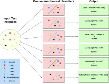
Moreover, we have also implemented an open set environment us-ing a series of support vector machines, where each SVM operates a one-versus-the-rest classification, with and without the use of known-unknown features.
We hope that the results achieved can further clarify the role of bis-pectral analysis in the distinction between real and fake speech and could lead to more research in the field of audio (and speech) forensics.
This work is organised as follows: in Chapter 1 we present some no-tions on features extraction and normalisation, dimensionality reduction techniques and classification algorithms that can be useful in order to understand the work we have done. Chapter 2 gives an overview on the state of the art as concerns multimedia forensics and speech synthesis techniques, other than describing few methods in literature that can be used to recognise real speakers from speech generated automatically by computing systems and artificial intelligence techniques. In Chapter 3 we will describe the methodology we have used in detail, while in Chapter 4 we will show the results of the open set and closed set classifications performed using the MK, UNET and MKU features, testing our models with a various and heterogeneous dataset of voices (both bonafide and spoofed speech signals). In Appendix A can be found the results of classi-fications performed using a convolutional neural network (CNN) applied to the modules of the bicoherences. In Appendix B are shown the results of experiments made using a U-Net trained on bonafide speech. Finally, in Appendix C we will show all the confusion matrices related to the closed set classifications that have been performed.
1
Theoretical Background
In this Chapter we will briefly introduce feature extraction and normal-isation and we will describe few techniques of dimensionality reduction.
Then, after an introduction on machine learning, will describe the problem of classification in detail. Moreover, we are going to analyse few different classifications techniques such as SVM, LR and RF, which we are going to use to classify our features, and we will show how to use CNNs and convolutional autoencoders to perform classifications.
Finally, we will explain what it means to perform an open set classifi-cation and we and we will introduce some metrics like confusion matrices, accuracy and receiver operating characteristic (ROC) curves, which will be useful in order to evaluate the performance of our classifiers.
1.1
Features extraction, features
normalisa-tion and dimensionality reducnormalisa-tion
In this Section we are going to introduce the concept of features ex-traction from multimedia content such audio files or images and we will present some post-processing techniques, like feature normalisation.
Moreover, we are going to describe few dimensionality reductions techniques, which will be used in order to visualise two different set of features extracted by the bicoherences , i.e. mean-kurtosis (MK) and mean-kurtosis-UNET (MKU) features, both in a 2D and a 3D space.
1.1.1
Features extraction and normalisation
Features extraction commonly refers to the set of techniques used to re-duce the dimensions of signals (and therefore the amount of data that needs to be processed by a digital system) selecting and computing vari-ables in order to maintain relevant information about the original data.
For example, if we have a signal consisting of temperature measure-ments in a room every minute, a possible feature that one may want to extract is the daily mean and variance of the temperature. This way we reduce the amount of data, keeping the relevant information about the temperature itself.
The most common features used in audio processing (and speech pro-cessing in particular) are basically three: the Mel-frequency cepstrum co-efficients (MFCCs), the linear prediction cepstrum coco-efficients (LPCCs) and the spectrogram.
In order to extract these features, usually the time-domain audio sig-nal y(k) is subjected to some pre-processing operations like segmentation and windowing. Segmentation consists in dividing the signal into small fragments, each one of which is processed on its own, while windowing is simply the multiplication of each segmented fragment for a window function; the most common window functions used in audio processing are rectangular window, Hamming window and Hann window.
Another common operation applied to audio signals, which is fre-quently involved as a fundamental step in feature extraction techniques, is the computation of the frequency representation of the signal itself, that is performed applying to the signal some implementation of the discrete Fourier transform (DFT), commonly referred to as fast Fourier transform (FFT).
Feature extraction is a crucial step in multimedia processing. How to extract ideal features that can reflect the intrinsic content of an image or audio signal as complete as possible is still a challenging problem in computer vision [5].
Once the desired features have been extracted, one may want to nor-malise them in order to change the range of values they assume. We are going to show two methods for features normalisation, which are the most commonly used in practice.
In the following we are going to use x and X to indicate respectively a vector or matrix that contains the features.
The first method is called min-max normalisation; it transform the features by scaling each feature to a given range as follows:
xscaled = a +
(x − min(x))(b − a)
max(x) − min(x) , (1.1) where x is the original feature vector, xscaled is the normalised vector,
a and b are the minimum and maximum values of the interval of values that the normalised features are going to assume, and min(x) and max(x) are respectively the minimum and maximum values of the original signal.
Usually, for features to be used in machine learning applications, one wants a = 0 and b = 1, such that the features are going to assume values in the interval [0, 1]. In that case the transformation becomes
x′scaled = x − min(x)
max(x) − min(x). (1.2) Another possible normalisation technique is called Z normalisation; it yields values that belong to the interval [0, 1], as follows:
x”scaled = x − µ σ , (1.3) with µ = ∑︁N i=1xi N (1.4) and σ = ⌜ ⃓ ⃓ ⎷ 1 N N ∑︂ i=1 (xi − µ)2, (1.5)
where N is the number of samples, µ, σ are respectively the mean and standard deviation, and xi is the i-th sample of the feature vector.
In the proposed system, the main feature extraction step corresponds to the transformation of speech audio signal into the bicoherence. Indeed bicoherences are supposed to retain all the relevant information from the original audio signals that can be used to classify the various classes of speech with respect to the synthesis method used to generate them. We will show how bicoherences are defined and how to extract them in Chapter 2. Moreover, we will extract additional sets of features from the bicoherences and these features will be used to perform our closed set and open set classifications; this latter feature extraction is useful to further reduce the amount of data we are going to work with.
1.1.2
Dimensionality reduction techniques
Dimensionality reduction is the transformation of data from a high-dimensional space into a low-high-dimensional space such that the low-high-dimensional representation retains some meaningful properties of the original data.
Working in high-dimensional spaces can be undesirable, for example for computational complexity reasons. Moreover, working in a two or three-dimensional space can be useful for visualizing the data by means of scatter plots.
In the following, we are going to describe three different methods for dimensionality reduction: principal component analysis (PCA), indepen-dent component analysis (ICA) and t-distributed stochastic neighbour embedded (TSNE). These techniques will be used to reduce the dimen-sionality of mean-kurtosis (MK) and mean-kurtosis-UNET (MKU) fea-tures in order to be able to visualise them in a 2D and 3D space, and see
how the different classes of speech that we are going to classify cluster in these spaces.
1.1.2.1 PCA
Principal component analysis (PCA) is one of the oldest and most widely used techniques for dimensionality reduction. PCA consists in finding new variables that are linear functions of those in the original dataset, that successively maximize variance and that are uncorrelated with each other. Finding such new variables, also known as the principal compo-nents (PCs), reduces to solving an eigenvalue/eigenvector problem. PCA as a descriptive tool needs no distributional assumptions and, as such, is very much an adaptive exploratory method which can be used on nu-merical data of various types [6].
Suppose we have n individuals, and for each of them we acquire ob-servations of p different variables. We can represent our initial dataset with an n × p data matrix X whose j-th column is the vector xj of
observations on the j-th variable.
We are looking for a linear combination of the columns of matrix X with maximum variance. Such linear combination is given by
p
∑︂
j=1
ajxj = Xa, (1.6)
where a is a vector of constants a1, a2...ap. The variance of any such
linear combination is given by
var(Xa) = aTSa, (1.7) where S is the sample covariance matrix associated with the dataset and the symbol T denotes the transpose operation.
Hence, identifying the linear combination with maximum variance is equivalent to obtaining a p-dimensional vector a which maximizes the quadratic form aTSa.
For this problem to have a well-defined solution, an additional restric-tion must be imposed, which involves working with unit-norm vectors, i.e. requiring
aTa = 1. (1.8)
The problem is equivalent to solve the well known eigenvalue/eigenvector problem given by
Sa − λa =0 ⇐⇒ Sa = λa (1.9) Thus, a must be a (unit-norm) eigenvector, and λ the corresponding eigenvalue, of the covariance matrix S.
In particular, we are interested in the largest eigenvalue, λ1 (and
corresponding eigenvector a1), since the eigenvalues are the variances of
the linear combinations defined by the corresponding eigenvector a: var(Xa) = aTSa = λaTa = λ. (1.10) Any p × p real symmetric matrix, such as a covariance matrix S , has exactly p real eigenvalues, λk (k = 1, ..., p), and their corresponding
eigenvectors can be defined to form an orthonormal set of vectors. The full set of eigenvectors of S are the solutions to the problem of obtaining up to p new linear combinations
Xak = p
∑︂
j=1
ajkxj, (1.11)
which successively maximize variance, subject to uncorrelatedness with previous linear combinations. These linear combinations Xak are
called the principal components (PCs) of the dataset [6]. 1.1.2.2 ICA
Another dimensionality reduction technique that we are going to intro-duce is independent component analysis (ICA). ICA is a linear trans-formation method in which the desired representation is the one that minimises the statistical dependence of the components.
ICA of the random vector x consists of finding a linear transform
s = W x (1.12)
such that the components si are as independent as possible, in the
sense of maximising some function F (s1, ..., sm) that measures
indepen-dence.
We can formulate the problem also in a generative way as follows: ICA of a random vector x consists of estimating the following generative model for the data:
x = As, (1.13)
where the components si in the vector s = (s1, ..., sn)T are assumed
independent, and the matrix A is a constant m × n "mixing" matrix. It can be shown that if the data follows the generative model, the Equa-tions (1.12) and (1.13) become asymptotically equivalent, and the natural relation
W = A−1 (1.14)
can be used with n = m.
The identifiability of the model can be assured by imposing the fol-lowing fundamental restrictions:
• All the independent components si with the possible exception of
one component, must be non Gaussian.
• The number of observed linear mixtures m must be at least as large as the number of independent components n, i.e. n ≥ m.
• The matrix A must be of full column rank.
The estimation of the data model of independent component anal-ysis (ICA) is usually performed formulating an objective function and minimising or maximising it.
An example of objective function is the likelihood: denoting by W = (w1, ...wm)T the matrix A−1, the log-likelihood takes the form
L = T ∑︂ t=1 m ∑︂ i=1 log fi(wiTx(t)) + T ln |det(W )|, (1.15)
where the fi are the density functions of the si (here assumed to be
known), and the x(t), t = 1, ..T are the realisations of x [7].
The log-likelihood can be maximised (for example using a classic gra-dient descent approach) in order to estimate the matrix W , which can be used to compute the independent components s thanks to Equation (1.12).
1.1.2.3 TSNE
The last dimensionality reduction technique that we are going to describe is the t-distributed stochastic neighbour embedded (TSNE). TSNE has been proposed by L. van der Maaten and G. Hinton [8] in order to offer a technique to convert an high dimensional dataset X = {x1, x2, ..., xn}
to a two or three dimensional dataset Y = {y1, y2, ..., yn} that can be
displayed in a scatter plot.
First of all we are going to introduce the stochastic neighbour embed-ded (SNE), and then we are going to explain the modifications to obtain the t-distributed SNE.
SNE starts by converting the high-dimensional Euclidean distances between data points into conditional probabilities that represent similar-ities. The similarity of data point xj to data point xi is the conditional
probability pj|i that xi would pick xj as its neighbour if neighbors were
picked in proportion to their probability density under a Gaussian cen-tered at xi. For nearby data points pj|i is relatively high, whereas for
widely separated data points, pj|i will be almost infinitesimal [8].
The conditional probability pj|i is given by
pj|i= e −||xi−xj ||2 2σ2 i ∑︁ k̸=ie −||xi−xk||2 2σ2i , (1.16)
where σi is the variance of the Gaussian centered on data point xi.
It is not likely that there is a single value of σi that is optimal for
all data points in the dataset, because the density of the data usually varies. In dense regions, a smaller value of σi is usually more appropriate
than in sparser regions. Since we are only interested in modeling pairwise similarities, we set the value of pi|i to zero.
For the low dimensional counterparts yiand yjof the high dimensional
points xiand xj it is possible to compute a similar conditional probability,
which we denote by qj|i; we set the variance of the Gaussian involved in
the computation of qj|i to √12, and we obtain the following:
qj|i=
e−||yi−yj||2
∑︁
k̸=ie−||yi−yk||
2. (1.17)
Again, since we are only interested in modeling pairwise similarities, we set qi|i = 0.
SNE aims to find a low dimensional data representation that mini-mizes the mismatch between pj|i and qj|i.
A natural measure of the faithfulness with which qj|imodels pj|iis the
Kullback-Leibler divergence. SNE minimizes the sum of Kullback-Leibler divergences over all data points using a gradient descent method.
The t-distributed SNE, has been introduced to solve problems like the difficulty to optimize the objective function of SNE and the so called "crowding problem" (for more information see [8]).
The cost function used by TSNE differs from the one used by SNE in two ways:
• It uses a symmetrised version of the SNE cost function with simpler gradients
• It uses a student-t distribution rather than a Gaussian to compute the similarity between two points in the low-dimensional space
1.2
Machine learning techniques and
classi-fication algorithms
The field of machine learning is concerned with the question of how to construct computer programs that automatically improve with experi-ence.
Most of machine learning processes can be divided into two phases: the learning phase and the performance measurement phase. The learn-ing phase is commonly known as "trainlearn-ing" (we say that a model is trained), and consists in learning new experience from data (which is called "training data" or "training set"); learning is the process of find-ing statistical regularities or other patterns of data [9].
The second phase consists in measuring the performance of the model after it has been trained; it is usually called "test", and is performed on
a dataset (called "test set") which has to be disjoint from the training set.
There are several types of learning, which differ w.r.t the way the model is trained. We are going to introduce four of them:
• The first one is the so called supervised learning, and consists of generating a function that maps the inputs to desired outputs, which are available during the training phase. The outputs are usually represented by labels on the training data [9].
• In opposition to supervised learning, we also have unsupervised learning, where the outputs are not available during the training phase. An example of unsupervised algorithm is clustering, which is the assignment of a set of observations into subsets (called clusters) such that observations within the same cluster are similar according to one or more predesignated criteria [10].
• Another form of learning is reinforcement learning (RL); in RL the algorithm learns a policy of how to act given an observation of the world. Every action has some impact in the environment, and the environment provides feedback that guides the learning algorithm. It has applications in many fields such as operations research and robotics [11].
• Finally, we have anomaly detection, which consists in analysing real world datasets in order to find which instances stand out as being dissimilar to all others. These instances are known as anomalies, and the goal of anomaly detection (also known as outlier detection) is to determine all such instances in a data-driven fashion. Anoma-lies can be caused by errors in the data, but sometimes they are indicative of a new, previously unknown, underlying process. In fact an outlier has been defined by Hawkins [12] as an observation that deviates so significantly from other observations as to arouse suspicion that it was generated by a different mechanism [13]. In the remaining of this Section, we are going to introduce the clas-sification problem (which is one of the most famous tasks in the field of machine learning); after that, we will describe some models such as support vector machine (SVM), logistic regression (LR), random for-est (RF), convolutional neural networks and convolutional autoencoder (and U-Net), which will be used in the following chapters to classify the features extracted from the bicoherences; moreover, we will discuss the problem of the open set classification. In the following Section we will introduce some metrics like confusion matrix, accuracy and ROC curve that are useful to measure the performance of a classification algorithm.
1.2.1
Classification problems
The goal of classification is to take an input vector x and to assign it to one of K discrete classes Ck for k = 1, ..., K. In the common scenario,
the classes are taken to be disjoint, such that each input is assigned to one and only one class. The input space is thereby divided into decision regions, where boundaries are called "decision boundaries" or "decision surfaces" [14].
Here we consider linear models for classifications, which means that the decision surfaces are linear functions of the input vector x.
1.2.1.1 Linear models for classification
Datasets whose classes can be separated exactly by linear decision sur-faces are said to be linearly separable. For two-class (or binary) problems, we can define a single target variable t ∈ [0, 1] such that t = 1 represents class C1 and t = 0 represents class C2. We can represent t as the
proba-bility that the class is C1, where t assumes only the extreme values of 0
and 1.
For K > 2 classes, we can define t as a vector of length K such that if the class is Cj, then all the elements tk of t are zero except element
tj, which takes value 1. For instance, if we have K = 5 classes, then a
pattern from class 2 would be given the vector
t = (0, 1, 0, 0, 0)T. (1.18) There are two different approaches to the classification problem. The simplest one involves constructing a "discriminant function" that directly assigns each vector x to a specific class.
A more powerful approach, however, models the conditional proba-bility distributions p(Ck|x)and uses these distributions to make optimal
decisions. In order to determine the probability distributions p(Ck|x)we
can proceed in two ways. One way is to model them directly, for example by representing them as parametric models and then optimising the pa-rameters using a training set (also known as probabilistic discriminative approach).
The other way is to adopt a probabilistic generative approach, in which we model the class conditional densities given by p(x|Ck)together
with the prior probabilities p(Ck) for the classes, and then we compute
the required conditional probabilities using the Bayes theorem p(Ck|x) =
p(x|Ck)p(Ck)
p(x) . (1.19)
We can model a prediction associated with input x as
where f() is a nonlinear function known as "activation function", w is the vector of coefficients to be determined called "weight vector" and w0 is a "bias" [14].
1.2.2
Support vector machine
In this section and the following ones we are going to describe some machine learning techniques that are useful to solve the classification problem and that we are going to use to classify the different classes of speech. We start from support vector machine (SVM).
Let us consider a linear model for the two-class classification problem: y(x) = wTϕ(x) + b, (1.21) where ϕ(x) denotes a fixed feature-space transformation, and b is the bias.
The training data set is composed by N input vectors x1, ..., xN with
corresponding target values t1, ..., tN where tn ∈ [−1, 1], and new data
points x are classified according to the sign of y(x).
We shall assume for the moment that the training dataset is linearly separable in the feature space.
The support vector machine (SVM) approaches the problem through the concept of the "margin", which is defined to be the smallest distance between the decision boundary and any of the samples. The decision boundary is chosen to be the one for which the margin is maximised.
The distance of a point xn to the decision surface is given by
tny(xn)
||w|| =
tn(wTϕ(x) + b)
||w|| . (1.22)
The margin is given by the perpendicular distance of the decision boundary to the closest point xn of the dataset, and we wish to optimise
the parameters w and b in order to maximise this distance. Thus the maximum margin solution is found by solving
arg max w,b {︃ 1 ||w|| minn [tn(w Tϕ(x) + b)] }︃ . (1.23) Direct solution of this optimisation problem would be very complex, and so we shall convert into an equivalent problem that is much easier to solve. To do this, we set
tn(wTϕ(x) + b) = 1 (1.24)
for the point that is closest to the surface. In this case all data points will satisfy the constraints
This is known as the canonical representation of the decision hyper-plane.
The optimisation problem then simply requires that we maximise ||w||−1, which is equivalent to maximising ||w||2, and so we have to solve
the optimisation problem
arg min
w,b
1 2||w||
2 (1.26)
subject to the constraints given by Equation (1.25).
This is an example of a quadratic programming problem, in which we are trying to minimise a quadratic function subject to a set of linear inequality constraints [14].
The points that lie on the maximum margin hyperplanes in feature space are called support vectors, and are the only one that will be retained in order to classify new data points. All other points, once the model is trained, can be discarded. This property is fundamental for the practical application of SVMs.
1.2.3
Logistic regression
The next classification model we discuss is logistic regression (LR), which is a probabilistic discriminative model.
In order to do that, instead of working with the original input vector x, we will work in the feature space using ϕ(x), which is a nonlinear transformation of the inputs.
All algorithms are equally applicable in the feature space. The re-sulting decision boundaries will be linear in the feature space ϕ, but will correspond to nonlinear decision boundaries in the original x space. Classes that are linearly separable in the feature space ϕ(x) need not be linearly separable in the original observation space x.
Consider a two-class problem. We model the posterior probability of class C1 as
p(C1|ϕ) = y(ϕ) = σ(wTϕ) (1.27)
with p(C2|ϕ) = 1−p(C1|ϕ). Here the σ is the logistic sigmoid function
defined by
σ(a) = 1
1 + e−a. (1.28)
This model is known as logistic regression (LR). For an M-dimensional feature space ϕ, this model has M adjustable parameters.
We can use maximum likelihood to determine the parameters of the logistic regression model. We can define an error function by taking
the negative logarithm of the likelihood, which gives the "cross-entropy" error function in the form
E(w) = − ln p(t|w) = −
N
∑︂
n=1
{tnln yn+ (1 − tn) ln(1 − yn)}, (1.29)
where yn= σ(an), and an= wTϕn.
For logistic regression there is no closed-form solution, due to the nonlinearity of the logistic sigmoid function. However, the error function is concave, and so it has a unique minimum.
This minimum can be found using an efficient iterative technique based on the Newton-Raphson iterative optimisation scheme. The algo-rithm that uses the Newton-Raphson iterative optimisation scheme to solve the LR problem is also known as iterative reweighted least squares. Additional information can be found in [14].
1.2.4
Decision tree and Random Forest
The next classification technique that we will introduce is called RF. We will first describe decision trees, and then we will explain how to combine them to obtain the RF.
1.2.4.1 Decision tree
Decision trees classify instances by sorting them down a tree from the root to some leaf node, which provides the classification of the instance. Each node of the tree specifies a test of some attribute of the instance, and each branch descending from that node corresponds to one of the possible values of this attribute. An instance is classified by starting from the root of the tree, testing the attribute specified by this node and then moving down the tree branch corresponding to the value of the attribute. This process is then repeated for the subtree rooted at the new node.
Decision tree learning is best suited to problems with the following characteristics:
• Instances are described by a fixed set of attributes and their val-ues. The easiest situation for a decision tree classifier is when each attribute takes on a small number of disjoint possible values. How-ever, extensions to the basic algorithm allow handling real value attributes as well
• The target function has discrete output values
Most algorithms that have been developed for learning decision trees are variations on a core algorithm that employs a top-down greedy search through the space of possible decision trees [15]. Some examples are the ID3 and C4.5 algorithms.
1.2.4.2 Random forest
Significant improvements in classification accuracy have resulted in grow-ing an ensemble of trees and lettgrow-ing them vote for the most popular class. In order to grow these ensembles, often random vectors are generated, that govern the growth of each tree in the ensemble.
In particular, for the k-th tree, a random vector θk is generated,
in-dependently on the past random vectors θ1...θk−1, but with the same
distribution; and a tree is grown using the training set and θk, resulting
in a classifier h(x, θk), where x is an input vector.
After a large number of trees is generated, they vote for the most popular class. We call these procedures random forests. More specifically, a RF is a classifier consisting of a collection of tree-structures classifiers {h(x, θk), k = 1...}where the {θk}are independent identically distributed
random vectors and each tree casts a unit vote for the most popular class associated with input x [16].
1.2.5
Convolutional neural networks
The next classification model we discuss is called artificial neural net-work or simply neural netnet-work (NN). NNs are also known as "multilayer perceptrons", which anyway is a quite misleading name: indeed, even if they are actually composed by many layers, each one of these layers can be seen as a logistic regression (LR) (instead of a perceptron).
The resulting model is significantly more compact and faster to eval-uate than a SVM having the same generalisation performance. However, the likelihood function, which forms the basis for the network training, is no longer a convex function of the model parameters.
With neural networks, we fix the number of basis functions in ad-vance, but we allow them to be adaptive, which means that we use para-metric forms for the basis functions in which the parameters values are adapted during training [14].
We start from the following linear classification model y(x, w) = f (︄ M ∑︂ j=1 wjϕj(x) )︄ , (1.30)
where f() is a nonlinear activation function. Our goal is to extend this model by making the basis functions ϕj(x) depend on parameters, and
then to allow these parameters to be adjusted, along with the coefficients {wj} during training.
Neural networks use basis functions that follow the same form as Equation (1.30), such that each basis function is itself a nonlinear func-tion of linear combinafunc-tions of the inputs, where the coefficients in the linear combinations are adaptive parameters.
In order to derive the basic neural network (NN) model, which can be described as series of functional transformations, first we construct M
linear combinations of the input variables x1, ..., xD of the form aj = D ∑︂ i=1 wji(1)xi+ w (1) j0 , (1.31)
where j = 1, ..., M and the superscript (1) indicates that the
corre-sponding parameters are in the first layer of the network. The parameters w(1)ji are called "weights", while the parameters wj0(1) are the "biases".
The quantities aj are known as "activations". Each of them is then
transformed using a differentiable nonlinear activation function h() to give
zj = h(aj). (1.32)
These quantities correspond to the output of the basis functions, and are called "hidden units". The nonlinear functions h() are generally chosen to be sigmoidal functions such as the logistic sigmoid.
The values zj are then again linearly combined to give "output unit
activations" ak= M ∑︂ j=1 w(2)kjzj + w (2) k0 (1.33)
where k = 1, ..., K and K is the total number of outputs. This trans-formation corresponds to the second layer of the network.
Finally, the output unit activations are transformed using a logistic sigmoid function for multiple binary classification problems or a softmax activation function for multiclass problems.
We can combine these various stages to give the overall network func-tion that, for sigmoidal output unit activafunc-tion funcfunc-tions, takes the form
yk(x, w) = σ (︄ M ∑︂ j=1 w(2)kjh (︄ D ∑︂ i=1 w(1)ji xi+ w (1) j0 )︄ + wk0(2) )︄ (1.34) where the sets of all weight and bias parameters have been grouped together into a single vector w. Thus the neural network model is simply a nonlinear function from a set of input variables {xi}to a set of output
variables {yk} controlled by a vectorw of adjustable parameters. The
process of evaluating Equation (1.34) is called "forward propagation" of information through the network. This model can be easily generalised adding more layers of processing, where each layer consists in a weighted linear combination followed by an element-wise transformation using a nonlinear activation function [14].
A convolutional neural network (CNN) is a neural network which comprises one or more convolutional layers. This kind of networks are particularly suitable to work with image data. In the convolutional layer
the units are organised into planes, each of which is called a "feature map". Units in a feature map each take inputs only from a small sub-region of the image, and all the units in a feature map are constrained to share the same weight values. Inputs values are linearly combined using the weights and the bias, and the result transformed by a sigmoid nonlinearity using Equation (1.30).
If we think of the units as feature detectors, then all of the units in a feature map detect the same pattern, but at different locations in the input image. Due to weight sharing, the evaluation of the activations of these units is equivalent to a convolution of the image pixel intensities with a "kernel" comprising the weight parameters.
The outputs of the convolutional units form the inputs to the sub-sampling layer (also known as pooling layer) of the network. For each feature map in the convolutional layer there is a plane of units in the subsampling layer and each unit takes inputs from a small receptive field in the corresponding feature map of the convolutional layer. These units perform subsampling. In a practical architecture there may be several pairs of convolutional and subsampling layers [14]. In Figure 1.1 is shown an example structure of a convolutional neural network used to perform a multiclass classification task.
Figure 1.1: Example structure of a convolutional neural network used for classi-fication. Taken from https://towardsdatascience.com/a-comprehensive-guide-to-convolutional-neural-networks-the-eli5-way-3bd2b1164a53.
In Appendix A you can find the results of both binary and multiclass classifications of the modules of the bicoherences (treated as images) using a simple convolutional neural network.
1.2.6
Convolutional autoencoder and U-Net
A convolutional autoencoder is a convolutional neural network, generally used to work with image data, which can be divided into two parts: an
"encoder" and a "decoder". The encoder part of the network takes the image as input and gives as output a compressed version of the image itself, while the decoder takes as input the compressed version (i.e. the output of the encoder) and gives as output a reconstructed image which is usually similar to the original one (See Figure 1.2).
Figure 1.2: Autoencoder structure.
The key aspect of autoencoders is that they can reconstruct better the class of images used in the training phase. For example, if an autoencoder is trained with images of dogs, than it will perform a better reconstruction when tested with images of dogs instead of images of other animals.
Usually the autoencoder is used for features extraction, anomaly de-tection or image segmentation. In [17] robust autoencoders used for anomaly detection are described and compared to PCA. In Chapter 3 we are going to describe a method for features extraction , while in Ap-pendix B we will describe a method for anomaly detection. Both of these methods involve the use of a complex convolutional autoencoder called U-Net, which has been initially used in [18] for image segmentation. The main difference between the U-Net and a traditional autoencoder is that in the U-Net some skip-connection (or concatenation) layers are present, which link deeper layers of the network to more shallow ones.
1.2.7
Closed set vs open set classification
We now introduce the problem of open set classification. In an open set environment, the aim is to both discriminate among some "known" classes, which are used to train the model, and to classify as "unknown" instances of the input space belonging to classes which have never been seen by the model during the training phase.
Following the definition in [19], three different kinds of data are in-volved in an open set classification:
• Known data: data belonging to known classes that the model has to correctly detect and classify; this is used for both training and test
• Known-unknown data: data available at training time but assumed as unknown in order to model unknown data at training time; this is used for both training and test
• Unknown-unknown Data: data only used to test the model with instances belonging to classes which have never been seen during the training phase.
In [20] you can find a method for open set classification that involves the use of neural networks.
In Chapter 3 we will describe a method to implement an open set environment using a series of support vector machines.
1.3
Confusion matrix, accuracy and ROC curve
In this Section we will introduce confusion matrices, accuracy and ROC curves, which are useful metrics when it comes to evaluate the perfor-mance of a classification algorithm.
1.3.1
Confusion matrix
Usually, when a classification has been performed, for each input xt
be-longing to the test set, two values are available: the true class it belongs t to and the predicted class that it has been assigned to ˆt.
From this information, we can build a table that allows visualization of the performance of the classification algorithm. In this table, each row represents the instances of the predicted class, while each column represents the instances of the actual class. For the case of two-class problems, we have a 2 × 2 matrix as in Figure 1.3, where the two classes are indicated as positive class (P) and negative class (N).
The elements that are contained in the matrix are the following: • True positive (TP): is the number of instances of the input vector
xt that belong to the positive class and were correctly classified as
positive.
• False positive (FP): is the number of instances of the input vector xt
that belong to the negative class and were misclassified as belonging to the positive class.
• False negative (FN): is the number of instances of the input vec-tor xt that belong to the positive class and were misclassified as
belonging to the negative class.
• True negative (TN): is the number of instances of the input vector xt that belong to the negative class and were correctly classified as
Figure 1.3: Confusion matrix for a two-class classification problem
In order to have a balanced matrix, it is recommended to test the model with an equal number of positive and negative instances. In that case we have the the sum of the elements of each column is constant.
A confusion matrix can be normalised dividing the elements of each column by the total number of elements belonging to each class. If the matrix is normalised, the elements in the matrix will assume values in the interval [0, 1], and moreover, we have that the sum of the elements of each column is exactly 1. Confusion matrices can also be used for classifications involving more than two classes. In that case we have a row (and a column) for each one of the classes.
1.3.2
Accuracy and other metrics
A number of other metrics are available that give an estimation of how well we are classifying the instances in the input vector xt. In the
follow-ing we are gofollow-ing to show four of them (i.e. accuracy, precision, recall and F1 score), and we consider the quantities defined in the previous section:
• Accuracy: The accuracy is defined as ACC = T P + T N
N , (1.35)
where N is the number of total instances in the input vector xt in
case the confusion matrix is not normalised, while it is the number of classes in case of a normalised confusion matrix.
• Precision: P RE = T P T P + F P. (1.36) • Recall: REC = T P T P + F N. (1.37) • F1 score: F 1 = 2 · P RE · REC P RE + REC . (1.38) The highest these metrics are, the better the model performs in the classification task. All of them take values belonging to the interval [0, 1]. In the following chapters we are going to use accuracy to evaluate the performance of our classifications.
1.3.3
ROC curve
Another method, together with confusion matrices, which is useful to visualise the performance of a classification algorithm, and that we are going to use in the next Chapters, is called receiver operating charac-teristic (ROC) curve. This is used specifically for binary classifications. The curve is a plot of the true positive rate (TPR), defined as
T P R = T P
p , (1.39)
where p is the number of instances belonging to the positive class P , versus the false positive rate (FPR), defined as
F P R = F P
n , (1.40)
where n is the number of instances belonging to the negative class N. Usually, given a ROC curve, it is desirable to compute the area under curve (AUC), which is a value that belongs to the interval [0, 1] that represents the area that lies under the curve, and is a metric of the probability that an instance is correctly classified.