Università degli Studi di Ferrara
Dottorato di ricerca in Fisica
Ciclo XXIVCoordinatore Prof. Filippo Frontera
Radiocarbon dating for
contemporary art: hardware
developments and measurements
Settore scientifico disciplinare FIS/07
Dottoranda: Tutor interno:
Caforio Lucia Anna
Prof. Calabrese Roberto
Tutor esterni:
Prof. Petrucci Ferruccio
Dott.ssa Fedi Mariaelena
Contents
Contents ... i
Introduction ... 1
Chapter 1 Radiocarbon dating ... 5
1.1 Basic principles ... 5
1.2 Variations of 14C in living organisms ... 7
1.3 Variations of 14C in atmosphere ... 9
1.3.1 Natural causes ... 10
1.3.2 Anthropogenic causes ... 11
1.4 How to perform radiocarbon measurements ... 13
Chapter 2 Accelerator Mass Spectrometry ... 17
2.1 Samples preparation for AMS measurements ... 17
2.1.1 The issue of contaminations and the extraction of the suitable fraction to date ... 18
2.1.2 The “standard” sample preparation protocol ... 19
2.2 Accelerator Mass Spectrometry at LABEC... 21
2.3 The Cs-sputter ion source ... 23
2.4 Analysis on the low energy side ... 25
2.4.1 54° electrostatic analyzer ... 25
2.4.2 The injection magnet ... 26
2.5 The accelerator ... 27
2.6 Analysis at high energy side ... 29
2.7 Detection of the rare isotope 14C ... 30
2.8 Reporting 14C data ... 31
Chapter 3 Hardware developments and new pre-treatment protocols ... 33
3.1 The new graphitization line ... 33
3.1.1 Accuracy tests performed using the new graphitization line ... 36
3.2 Upgrade of the AMS beam line ... 39
3.2.1 Accuracy tests of the upgraded AMS beam line ... 42
3.3 New pre-treatment protocols ... 45
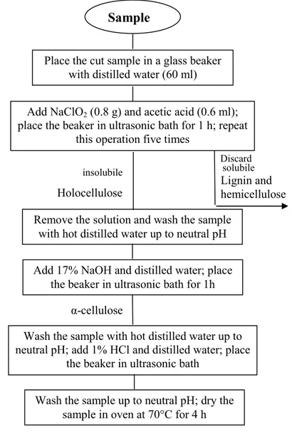
3.3.1 Alpha cellulose extraction ... 45
Chapter 4 Radiocarbon measurements on samples of the 20th century ... 53
4.1 The “local” bomb peak curve ... 53
4.2 Measurements on paper samples... 55
4.2.1 Newspaper samples ... 56
4.2.2 Fine paper samples ... 60
4.3 Measurements on canvas samples... 64
4.3.1 Textile fibres in modern and contemporary art ... 65
4.3.2 Canvas samples of the period 1900-1950 ... 69
4.3.3 Canvas samples of the bomb peak period ... 71
Chapter 5 Case studies: dating a restored painting and identifying a fake... 75
5.1 A restored painting ... 75
5.2 A forgery of a contemporary artwork ... 81
Conclusions ... 85
Introduction
The research developed during my PhD can be inserted within the activities of the Archaeometry Laboratory of the Ferrara Physics Department. In this laboratory, the artworks of historical-artistic interest are studied using non invasive and non destructive methods for diagnostic purposes and for a support to the work of the restorers, in order to identify e.g. the executive technique and the pigments utilized by the artists. In more recent years, the same methods have been also applied to investigate contemporary paintings (typically dated back to the period since the end of the 19th century until present). In fact, a rising interest has concerned this kind of artworks, given the necessity to characterize the new used materials to preserve these works of art by the natural and fast deterioration.
In addition, concerning contemporary art, it is well known that an important aspect, mainly in the trade field, is the authentication and so the identification of fakes. A simple analysis of the artistic style cannot sometimes be sufficient to solve these issues, while the support of scientific analyses, like that provided by a robust dating technique, is often required. In this framework, during my PhD, the capability to solve authentication issues by radiocarbon dating in an univocal way has been tested.
Radiocarbon (14C) is surely the principal radiometric method to study the past and in particular to date organic archaeological findings. However, since the end of the 1960s, radiocarbon has been also applied to forensics, initially in biological and medical fields, but also in archaeometry to identify forgeries of ancient artworks. The possibility to use 14C for the most recent samples is given by the so-called Bomb Peak. By this expression, the huge increase of the radiocarbon concentration in atmosphere after the Second World War is usually addressed. Actually, in the late 1950s and early 1960s, as a consequence of hundreds of nuclear weapon tests, large amounts of neutronswere produced in the atmosphere, thus significantly increasing the radiocarbon production rate. This artificial 14C input caused not only a global increase of the 14C/12C ratio in the atmospheric CO2 but also in all the other
reservoirs, i.e. in the oceans and in the biosphere. The increase was so large that the atmospheric radiocarbon concentration was almost doubled in less than 10 years. Then, after 1963, when the Nuclear Non-Proliferation Treat was signed, the 14C concentration started to
decrease due to the rapid exchanges with the carbon reservoirs. This is just the peculiar trend of the 14C concentration that is exploited in forensics to date samples with a very high precision.
During my PhD, to verify the possibility to date by radiocarbon contemporary artworks showing advantages and limits of the method, I have measured the 14C abundance in many paper and canvas samples of the 20th century. These materials were chosen because they represent the most common supports for artworks. All the samples were also carefully analysed by other techniques (Scanning Electron Microscopy, Fourier Transform Infrared Spectroscopy and Attenuated Total Reflectance Spectroscopy) to study the raw materials and their state of preservation, allowing us to choose the better protocol for the sample preparation (i.e. all the procedures to convert any sample to be dated to the proper chemical form needed for the measurements).
All the radiocarbon measurements were performed by Accelerator Mass Spectrometry (AMS) at INFN-LABEC (Laboratorio di Tecniche Nucleari per i Beni Culturali) in Florence, where a 3 MV Tandem accelerator is installed. Sample preparation to convert the samples to the graphite pellets for the AMS measurements was performed at LABEC as well. During my PhD, I have been also involved in the upgrade of the experimental set-up.
In the first chapter of this thesis, the basic principles of radiocarbon dating are described; in particular, the attention is focused on the natural and the anthropogenic causes that have affected the radiocarbon concentration in all living organisms during the centuries. In brief, the main reasons of the use of Accelerator Mass Spectrometry to perform radiocarbon measurements are also discussed.
In chapter 2, the features of AMS are described in detail. First, the standard sample preparation procedure (pre-treatment, combustion and graphitization process) necessary to obtain a graphite sample to be measured is presented. In particular, the need of the pre-treatment is due to the presence of possible contaminations in the sample to be dated; the specific case of contamination by dead carbon is mentioned, since this is the case that can be found when dealing with contemporary art samples. The 3 MV Tandem accelerator installed at LABEC is also explained; the AMS beam line is shown with reference to radiocarbon measurements.
In chapter 3, all the improvements in the experimental set-up developed during my PhD are presented. The new graphitization line and the upgrades of the AMS beam line are
described. Concerning new chemical pre-treatments, the new alpha cellulose extraction procedure and the new chloroform-based protocol for restored samples are reported.
In the fourth chapter, the radiocarbon measurements performed on paper and canvas samples of the 20th century are shown. Thanks to these measurements, the advantages and the limits of radiocarbon dating are highlighted.
In the last chapter, two case studies that demonstrate the feasibility of using radiocarbon dating applied to art are presented. The first case concerns the application of the new chloroform-based pre-treatment on a restored painting; as for the second case study, the identification of a forgery of a contemporary artwork is shown.
Chapter 1
Radiocarbon dating
In the mid of 1940s, studying the effects of cosmic rays on the earth and the earth’s atmosphere, Willard Libby put the bases of a new dating method based on the measurement of the residual abundance of a cosmogenic isotope: 14C (or radiocarbon). For this research, in 1960, he received the Nobel Prize in chemistry. Nowadays, radiocarbon dating represents one of the most important techniques to investigate the past. It has been used especially by archeologists to study the human evolution, but it has been also applied to others fields, such as geology, biology, art and forensics. In this chapter, the basic principles of radiocarbon dating are discussed.
1.1 Basic principles
Carbon is one of the most abundant elements on earth. In nature, there are three natural carbon isotopes. 12C and 13C are both stable and correspond to the 98.9% and 1.1% of the carbon on earth, respectively. 14C is present in a very small concentration and it is the only unstable isotope. It decays via beta emission to 14N with a half life T = 5730±40 years 1/2
[God1962].
Fig 1.1 Scheme of the radiocarbon decay.
14C is produced in the upper layers of the atmosphere by interaction of thermal neutrons
C
p
n
N
14 14(
,
)
(1.1)14C atoms rapidly combine with oxygen to form carbon dioxide. Considering the
radiocarbon half life and its fast production rate, the decayed radiocarbon is promptly compensated by natural continuous production; in this way, the 14C concentration in atmosphere can be considered constant, of the order of 1.2·10-12. Moreover, CO2 spreads over
the atmosphere and dissolves into the oceans. It enters also in the biosphere via e.g. photosynthesis in plants and nutrition in animals. A dynamic equilibrium is established between living organisms and the environment where they live, so that in all of these organisms the same 14C concentration as in the atmosphere is present.
When an organism dies, if we can consider it as a close system, this concentration starts to decrease due to radioactive decay. Assuming that the radiocarbon concentration in atmosphere has been constant in the past and it is the same in terrestrial and marine organisms, the residual radiocarbon concentration 14R(t) after a period t from the death is in
agreement with the radioactive law:
t total
e
R
C
C
C
C
t
R
14 0
12 14 14 14(
)
(1.2)In the equation (1.2), 14R0 is the radiocarbon concentration at the moment of death and τ is
the 14C mean life (= T1/2/ln2). Adopting for 14R0 the conventional value of 1.2·10-12, i.e. the
radiocarbon concentration in atmosphere in a year chosen as reference, namely AD 1950, and for τ the value of 8033 years (the so-called Libby mean life), we can define the conventional radiocarbon age tRC as:
)
(
ln
14 0 14t
R
R
t
RC
(1.3)The conventional radiocarbon age is expressed in years Before Present (years BP), where Present is 1950. 1950 was chosen as reference year partly for historical reasons (in that period, the first experimental results were published), but also because after this year the atmospheric radiocarbon concentration started to considerably change due to nuclear weapon
tests (see paragraph 1.3.2).
The age obtained from the equation (1.3) is not the true age of the sample, because some of the assumptions used to calculate tRC are true only as a first approximation (e.g. the
hypothesis according to which radiocarbon concentration in atmosphere has been constant in the past and it is equal in all organisms). In the next paragraphs these assumptions are discussed.
1.2 Variations of
14C in living organisms
When the conventional radiocarbon age (1.3) is defined, it is supposed that all living organisms are characterized by the same 14C concentration as the atmosphere. Actually, there are some alteration effects, depending on different carbon uptake paths and the environment where the organisms live, that may affect the radiocarbon concentration. The principal consequence of these effects is a discrepancy between the measured 14C concentration and the expected value.
One of the most important effects is known as isotopic fractionation, which is characteristic of many biological and chemical processes in which the isotopes of the same element are assimilated in different ways by living organisms; in particular, the lightest isotopes are preferentially taken up. In the case of processes involving the carbon isotopes, this means that 12C is better absorbed than 13C and 14C by the growing plants or animals. If the measured 14C concentration in a sample is very different with respect to the atmospheric value, the dated organisms will appear to be older or younger. In order to correct this effect, being 14C radioactive, the 13C/12C ratio is measured in all samples, since these two isotopes are stable and the variations of their abundances can be attributed only to fractionation.
The fractionation of 13C relative to 12C in a sample is defined as
1000
/
/
/
12 13 12 13 12 13 13
VPDB VPDB sampleC
C
C
C
C
C
C
(1.4)where (13C/12C)sample and (13C/12C)VPDB are respectively the isotopic ratio in the sample and
in the standard VPDB (Vienna Peedee Belemnite), a limestone fossil from a crustaceous formation in South Carolina (USA) [Cop1994]. Assuming the relationship between 13C
fractionation and 14C, demonstrated in [Cra1954], it is possible then to correct the measured 14C/12C ratio: 1000 25 2 1 13 , 12 14 , 12 14 sample meas sample corr sample C C C C C
(1.5)In the equation (1.5), by international convention, the δ13C
sample baseline is fixed at -25‰
with respect to VPDB; this value corresponds to the mean isotopic fractionation of terrestrial wood.
In Figure 1.2, the δ13C of several materials are reported.
Fig 1.2 Overview of isotopic fractionation mean values in different natural compounds (reproduced from
[wIA2011].
An effect concerning marine organisms is the so-called reservoir effect. In the oceans, the atmospheric carbon dioxide is exchanged only on the surface layers of water, which are so rich in 14C. Then, thanks to marine flows, CO2 absorbed from the atmosphere can diffuse into
the deep waters. In the meantime, the upwelling mechanism contributes to mix the waters, moving upwards the “old” waters, depleted in radiocarbon, and thus diluting the 14C concentration present in the ocean surface. Hence, as effect of these processes, the marine
samples are characterized by a lower radiocarbon concentration than terrestrial samples, showing a typical apparent ageing of about 400 years (as an average).
1.3 Variations of
14C in atmosphere
In order to test the new radiometric dating method, Libby performed the first measurements on samples of known ages, in particular archaeological findings from ancient Egypt. During the 1950s, when the instrumental set ups (in particular, the detection systems) and so the accuracy of the measurements improved, a discrepancy between the measured radiocarbon ages and the historical Egyptian chronology was eventually noticed [Lib1960, Bow1990]. This fact could be explained by assuming a variation of the 14C concentration in atmosphere during the centuries, as it was verified by measuring the radiocarbon content in samples that could be dated also by independent methods, i.e. tree rings.
Trees grow up annually, usually adding a single ring to their trunk each year. This ring is the only one that exchanges carbon with the atmosphere, reaching an equilibrium condition; thus it stores the 14C concentration of the year in which it “lived”. In this way, the measurements of 14C concentrations in tree rings allow recording the atmospheric variations year by year. A calibration curve, in which measured radiocarbon ages are correlated to calendar ages, can be so arranged, by comparing the radiocarbon data to the dates obtained by independent method e.g. dendrochronology1. In fact, the first recommended calibration curve, which covered the time period BC 2500 – AD 1950, was obtained by combining radiocarbon ages with dendrochronologically dated wood [Pea1986, Stu1986]. Since then, new materials have been dated, now extending the calibration curve back to about 50.000 years BP; these materials are corals, foraminifera and varve lake sediments, dated by other independent methods, such as that based on Uranium/Thorium series. In Figure 1.3, a portion of the recently updated calibration curve, IntCal09, is shown [Rei2009].
1 Dendrochronology is a dating method based on the analysis of patterns of tree rings. Measuring e.g. the width and the density of tree rings, master chronologies for different trees species are obtained. Therefore, comparing the sample rings with the corresponding master chronology, an absolute dating of wooden samples is achievable.
18000 19000 20000 21000 22000 23000 24000 25000 26000 27000 28000 20000 21000 22000 23000 24000 25000 26000 27000 28000 29000 30000 calendar age BC ra d io c a rb o n a g e B P
Fig 1.3 Portion of IntCal09, the atmospheric calibration curve [Rei2009]. On the y axis the radiocarbon age,
expressed in years BP, and on the x axis the calendar age are reported.
Observing the Figure 1.3, we can notice that the calibration curve is not a monotonic function and it has not a constant trend.
1.3.1 Natural causes
The measured variations of the 14C concentration in atmosphere are due both to natural and to anthropogenic causes that are described in the following.
Radiocarbon production in atmosphere is affected by the earth magnetic field, which is latitude dependent. Indeed, being charged particles, cosmic rays are deflected by magnetic field; as a consequence, the production rate of 14C atoms on earth is not constant with the latitude; for example, a bigger 14C concentration is present at the poles than at equator. This effect is minimized by a rapid mixing in the atmosphere due to the air fluxes that lead to uniform the 14C concentration [Kor1980, Bow1990].
However, changes of the magnetic field in the past, such as reversals and polarity excursions, have strongly influenced the abundance of radiocarbon in atmosphere. The relationship between the magnetic dipole moment changes and the 14C activity has been demonstrated by several investigators [Ste1983], finding a predominant trend with a periodicity of about 8000 years.
In addition, other short-term variations of the radiocarbon concentration are due to the solar activity. Actually, the variation of the solar activity causes a change of the flux of
protons on earth. Following this process, the quantity of neutrons, responsible of the 14C atoms production, is not constant; thus, the radiocarbon production rate is variable with time. This effect was demonstrated in several studies [Kor1980, Sue1986, Der1995], just measuring the 14C concentration in tree rings, as also explained in the previous paragraph. Generally, the solar variations have a periodicity of about 200 years and cause the so-called wiggles (fluctuations over short term calendar length). An 11-year sunspot activity cycle is registered too, but its effect has been estimated unimportant [Sue1986].
1.3.2 Anthropogenic causes
14C variations in atmosphere have been caused not only by nature, but also by human
activity, i.e. principally by the industrialization process and by the nuclear weapon tests. Since the beginning of the 19th century, the continental Europe, in particular Germany and England, has been involved in the industrial revolution process. Appreciable amounts of carbon dioxide began to be added to the atmosphere thanks to the combustion of fossil fuel [Rev1957]. The rate of combustion has continuously increased causing a dilution of the natural radiocarbon concentration in the atmosphere and, as a consequence, a decreasing of the 14C/12C ratio in all carbon reservoirs (e.g. oceans) and in all living organisms. This effect was discovered by Hans Suess in 1953 [Lev1989]. In order to estimate this so-called Suess effect, measurements were performed again on tree rings [Aws1986, Paw2004]. The industrialization process has been not concluded yet, so that this effect is still present in all living organisms [Lev2000].
Another anthropogenic effect is known as Bomb Peak (or Bomb Spike). In the late 1950s and early 1960s, as a consequence of hundreds of nuclear weapon tests, large amounts of neutrons were produced in the atmosphere, thus significantly increasing the radiocarbon production rate. This artificial 14C input caused not only a global increase of the 14C/12C ratio in the atmospheric CO2 but also in all the other reservoirs (mainly the oceans and the
biosphere). The increase was so large that the atmospheric radiocarbon concentration was almost doubled in less than 10 years. After 1963, when the Nuclear Non-Proliferation Treaty was signed [wFa2011], the 14C concentration started to decrease due to the rapid exchanges with the carbon reservoirs. In Figure 1.6, the atmospheric radiocarbon concentration is reported as a function of the year: the huge increase starting since 1955 is evident. In the figure, four different curves are shown, each of them related to a defined region of earth.
90 100 110 120 130 140 150 160 170 180 190 200 1940 1950 1960 1970 1980 1990 2000 years AD p M C Bomb04NH1 Bomb04NH2 Bomb04NH3 Bomb04SH
Fig 1.6 Atmospheric 14C curves relative to the four zones of earth. The 14C concentrations are expressed in pMC; reproduced from [Hua2004].
The NH1 zone covers the area from ~40°N to the North Pole; it is the zone where Italy (except the Sicily) is included. The NH2 zone extends from ~40°N to the summer maximum position of the summer so-called Intertropical Convergence Zone (ITCZ2); the NH3 zone covers the area from ITCZ to the equator; the SH zone is referred to the Southern hemisphere (see Figure 1.7).
Fig 1.7 World map showing the four zones; reproduced from [Hua2004].
Slight differences in the radiocarbon concentrations in atmosphere among the four different zones can be noticed in Figure 1.6. The highest 14C level was registered in northern
2 ICTZ (Intertropical Convergence Zone) is a zone close to the Equator where winds originating in the northern and in the southern hemispheres come together.
mid to high latitudes, while in the subtropics and mid-latitudes the level was lower. Nevertheless, the major number of nuclear weapon tests was carried out in the Pacific Ocean at different latitudes. Probably, these differences can be due to a bigger ocean surface in the southern hemisphere, contributing to a shorter residence time of 14C in the atmosphere than in the northern hemisphere.
The characteristic trend of the bomb peak curve allows us to date samples with a very high precision and permits thus the use of radiocarbon dating for forensics applications, for instance in biology and medicine to study the reproduction rate of the cells [Tun2004, Wil2000, Zop2004]. The Bomb peak curve can also be a very useful instrument in archaeometry, and in particular to recognize fakes of ancient artworks [Kre2004]. This PhD work has risen from the idea to use the bomb peak to also investigate contemporary artworks, realized in the 20th century. In the literature, not many applications on this topic are reported [Kei1972, Zav2004]. The advantages and the limits of using radiocarbon for such purposes are presented in this thesis, where measurements performed on different materials collected from objects of artistic interest of the 20th century are shown.
1.4 How to perform radiocarbon measurements
Only organic samples can of course be dated by radiocarbon. Among all the materials, we can here mention bone, charcoal, wood, textile, paper and papyrus. These samples generally are of archaeological and of historical-artistic interest. Since the radiocarbon dating method requires that a sample has to be collected from the object to be dated, the importance of choosing a measurement technique that needs just a small quantity of sample is mandatory. During the time, different methods for radiocarbon dating have been tested. The first measurements were done using the β counting method. Although this technique is not relatively very expensive and allows performing the measurements quite easily, a not positive aspect is the fact that it requires samples that are quite big. On the contrary, considering the typical historical value of the objects to be measured, the necessity to take a small sample is fundamental.
Nowadays, in most of the laboratories, radiocarbon measurements are performed using the technique known as Accelerator Mass Spectrometry (AMS) [Tun1998], which is based on the use of a particle accelerator coupled to selective filters like those characterizing a mass spectrometer.
In general, the basic principle on which mass spectrometry (MS) is based is that ions having the same energy and charge are deflected in a magnetic field with different trajectories according to their mass. The samples are ionized (usually as positive ions) and accelerated to energy in the range of 1-10 keV. Measuring the relative abundance of the isotopes, quantitative information about the sample can be obtained. In this range of energy the sensitivity is about 10-10. Limitations to the sensitivity are also caused by the background counts, produced by interaction with apertures, walls and residual gas into the spectrometer [Fin1993].
Since the relative abundance of 14C is only about 1.2·10-12 (in modern samples) and the
detection of this isotope is complicated by the presence of isobaric interferences that are more abundant than the 14C itself, the typical sensitivity of traditional mass spectrometry is too low to permit the radiocarbon measurements. Indeed, concerning 14C, one of the most important isobars is the stable isotope 14N (see Figure 1.8), representing about 78% of the earth’s atmosphere.
Fig 1.8 Portion of the table of nuclides showing carbon isotopes and their neighbours [wAt2000]
There are also molecular interferences. Indeed, 12C and 13C easily combine with H atoms, forming the 12CH2 and 13CH molecules; these molecules are characterized by a difference in
masses extremely small.
The limits of traditional MS are overcome by Accelerator Mass Spectrometry. It represents a very useful method for radiocarbon measurements because:
using a negative ion source, it is capable to suppress isobaric interferences that do not form negative ions (in the case of radiocarbon, the suppressed interference is 14N);
thanks to the stripping process at the high voltage terminal of the accelerator, the molecular interferences (i.e. 12CH2 and 13CH) are suppressed;
working in a range of energies of the order of MeV allows identifying and separating the ions of interest from any residual atomic and/or isobaric interferences.
Thanks to these characteristics, AMS is able to reach a very high sensitivity (10-15); in addition, the efficiency of the method allows measuring samples with masses of the order of few milligrams.
Chapter 2
Accelerator Mass Spectrometry
This chapter is divided into two sections. In the first part, the procedure to obtain a sample for 14C-AMS measurements is explained; in the second part, the Tandem accelerator installed at INFN-LABEC (LAboratorio di tecniche nucleari per i BEni Culturali, Florence), where the measurements for this thesis were performed, is presented; in particular the AMS beam line is described.2.1 Samples preparation for AMS measurements
With the term samples preparation, all the physical-chemical procedures used to treat the samples to be dated and the graphitization process employed to convert them into graphite (the chemical form for the sample to be inserted in the source of accelerator3) are meant. In particular, samples preparation aims at the removal of the contaminants that may affect the measurements and at the extraction of the suitable organic fraction to be dated.
The typical masses collected for a radiocarbon AMS measurement are of the order of some tens of mg (see Table 2.1), bigger than the mass of the final graphite pellet that will be used for the measurement itself (typically of the order of some hundreds of μg). Indeed, during the different steps of sample preparation, a mass loss has to be taken into account. This mass loss depends on the type of materials and on the percentage of contaminants present in the samples.
3 For radiocarbon measurements, the most of the AMS facilities are equipped with ion sources for solid state samples. There are also hybrid ion sources that are able to measure also samples in a gaseous state. For instance, this type of sources is advantageous in measuring very small samples (about ~50µg) [Ruf2010].
Materials Masses (mg) Charcoal 20-40 Wood 20-30 Textile 30-40 Paper 20-30 Bone 1000
Table 2.1 Order of magnitude of the typical masses of collected samples for radiocarbon measurements for
different materials (before any treatment).
2.1.1 The issue of contaminations and the extraction of the suitable
fraction to date
In general, there are two different kinds of contaminations: contamination by “dead” carbon (e.g. carbonates) contamination by “modern” carbon (e.g. humic acids).
The term “dead” carbon is referred to all materials containing a 14C concentration that is well below the sensitivity limit of the measurement technique, thus appearing infinitively old; as a consequence, if a percentage of this contamination is present in the samples, their radiocarbon age will appear older than the true age. In the case of “modern” carbon, the effect on radiocarbon age is opposite. Indeed, adding a contamination with a 14C content equal to the present concentration in atmosphere, the measured samples will appear younger.
More specifically, the case of contamination by dead carbon is here explained, since this is the situation that may occur when dealing with dating findings of historical-artistic interest, such as those analysed in this thesis. The relationship between the measured radiocarbon concentration 14Rmeas and the fraction x of dead carbon contamination in the sample is:
true meast
R
x
R
exp
1
1
0 14 14 (2.1)
x
t
R
R
t
true meas app
ln
14
ln
1
0 14
(2.2)Hence, a dead carbon contamination of 1% introduces an absolute discrepancy on the measured radiocarbon age of 80 years. This contamination effect is independent of the true age of the sample, but, obviously, this effect is more significant for recent sample.
Contaminations can be natural and/or anthropogenic. The natural contaminations, such as traces of humic acids from the soil and of calcium carbonates dissolved in groundwaters, are especially characteristics of archaeological findings (i.e. bones, charcoals and seeds) that had been buried for several centuries. Being a non endogenous carbon fraction, these traces have to be removed to exclude any contamination effect on measured radiocarbon ages. As far as the anthropogenic contaminations are concerned, the materials and the chemical products used by restorers to consolidate historical objects can be taken into account. These products are usually obtained by industrial processes and are synthesized by hydrocarbons, which are obviously fossil carbon based. These products are thus sources of contamination by dead carbon and their incomplete removal can affect the measured radiocarbon age.
As introduced above, the other goal of the sample preparation is the extraction from the sample of the appropriate fraction to be dated. To illustrate this, the case of bone can be reported as an example. Bone is formed by two fractions: an organic fraction, consisting in the collagen protein (more subjected to degradation), and an inorganic fraction, essentially calcium hydroxyapatite (Ca5(PO4)3(OH)). Both components contain carbon, so, in principle,
both of them might be dated. In practice, the inorganic fraction can be contaminated by calcium carbonates originated from percolating groundwater; hence, in order to exclude the contribution of non endogenous carbon, this fraction is removed using a chemical pre-treatment and only the collagen is extracted and dated. Collagen is only a small fraction in bone. This is the reason of the use of about 1 g of bone samples to be treated [McC2010, Tal2011].
2.1.2 The “standard” sample preparation protocol
At INFN-LABEC, a sample preparation laboratory is present; here the samples are subjected to a standard protocol (pre-treatment, combustion, graphitization process). In this way, the samples are converted into graphite powder.
Initially the sample undergoes a physical treatment in order to remove the most external layers that might be more contaminated and might thus affect the radiocarbon dating. This operation generally consists in scratching the sample surface, using tweezers and a scalpel. If necessary, an observation under optical microscope can be useful.
Afterwards, the sample is treated with chemical reagents. The most suitable chemical protocol has to be chosen according to the sample material and to the fraction that we would like to extract and date. In most cases, a simple protocol, called ABA (acid-base-acid), is applied; it consists in a series of baths in acid and basic solution [wHi99]. The acid solution (typically, at LABEC, hydrochloric acid 1M) allows dissolving carbonate residues. The bath in alkaline solution (typically, at LABEC, sodium hydroxide 0.1M) has the role to eliminate humic acids. Finally, a further bath in acid is necessary to remove traces of atmospheric CO2
entered in the solution in the previous step. The samples are then dried in oven.
Once the sample is clean, it is necessary to extract and isolate only carbon. For this purpose, the sample is oxidized so that carbon is collected as gaseous CO2. At LABEC, this
step is achieved by combusting the sample in an elemental analyzer (EA). The combustion process takes place in a furnace at a temperature of about 1100°C. The gas flows in a quartz column filled with different chemical materials (chromium oxide, reduced copper, silvered cobaltus oxide). As a consequence, when a typical organic sample is burnt, at the exit of this column, the gas is composed by N2+CO2+H2O, while any sulphides are absorbed. Then, the
three gaseous components pass through a gaschromatographic column, a spiral filled with an adsorbent material that adsorbs and desorbs the gases with different retention time according to their molecular weight. Therefore, the three gases come out of the column separately. At the exit of the gaschromatographic column, a thermal conductivity detector (TDC) is present. Three signals corresponding to each gas are detected. The area of each peak is proportional to the quantity of gas in the circuit. In Figure 2.1 a typical chromatogram acquired after gaschromatographic column is shown.
Fig 2.1 Chromatogram acquired for a cyclohexanone sample (C12H14N4O4): the three gaseous components are
well time-separated.
During the time interval t0-t1 (see Figure 2.1), only the gaseous CO2 is transferred into the
graphitization line, where it is converted to graphite, exploiting the reaction:
O
H
C
H
CO
2
2
2
Fe,
600
C
2
2 (2.3)In the reaction 2.3, carbon dioxide interacts with hydrogen at high temperature (about 600 °C) in the presence of iron powder as catalyst. The typical masses of the graphite samples prepared at LABEC (and for this work) are of the order of 700 µg. More details on the graphitisation line and on the principal steps of the graphitisation process will be given in chapter 3.
The iron and graphite mixture is then pressed into an aluminum target holder that is inserted in the source of the accelerator.
2.2 Accelerator Mass Spectrometry at LABEC
In the next paragraphs, the Tandem electrostatic accelerator installed at INFN-LABEC in Florence are explained. In particular, the AMS beam line will be described, with reference to radiocarbon measurements.
The 3 MV Tandem accelerator was produced by High Voltage Engineering Europe (HVEE) and it was installed in 2004 [Fed2007]. It is equipped to perform both AMS and Ion Beam Analysis (IBA) measurements.
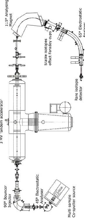
In Figure 2.3 a schematic layout of the AMS beam line is shown.
Fig 2.3 Schematic layout of the AMS beam line at the Tandem electrostatic accelerator of INFN-LABEC
(the two other independent ion sources and the switching magnet to the beam lines dedicated to IBA measurements are not shown).
2.3 The Cs-sputter ion source
The ions injected into Tandem accelerators have a negative charge. The typical requirements for an AMS solid samples ion source are high stable currents, high efficiency, low memory effects, rapid sample switching and isobaric separation [Kil1997]. In particular,
the high stable currents are important to reduce systematic errors especially when rare and abundant species are sequentially analyzed;
the high efficiency is related to the possibility to measure very small samples;
the low memory effect is necessary to guarantee the measurements in series of the samples minimizing cross contamination effects;
the possibility to switch the samples can reduce the measuring time;
the isobaric interferences due to particles that do not form negative ions can be suppressed.
The ion source installed on the AMS beam line at LABEC is of the Cs-sputter type.
As it is discussed in paragraph 1.4, the source acts as a filter to suppress the interference of nitrogen, since the nitrogen electron affinity is -0.07 eV.
In order to extract a negative beam from the sample (also called target), the graphite is bombarded by positive Cs ions. Cs is stored in a reservoir, which is heated up to about 75ºC; in this way, the vapours are released and come into contact with the spherical surface of the ionizer that is kept at about 1100 ºC. As a consequence of thermal ionization, positive Cs ions are formed. The Cs ions are accelerated on the sample surface thanks to a voltage of -7 kV (this voltage is called cathode voltage Vcat). The positive ions hit the sample graphite,
sputtering atoms and molecules from the surface. Since the sample is cooled, a thin Cs layer is condensed on its surface, so that when the molecules and the atoms pass through this layer, they can acquire electrons, becoming negative. The most probable charge state is q=-1. Being the target at a negative potential with respect to ground (-35 kV), the ions are extracted from the source through the small central hole (~ 5 mm) of the ionizer. At the exit of the source, the energy Einj of the negative ions is equal to Einj=q(Vext+Vcat), where q is -1, Vext is the voltage
difference between the ionizer and the exit of the source, kept at -28 kV, and Vcat is -7kV.
Extraction insulator Cathode insulator Potential Ground -28 KV -35 KV Extraction electrode Ionizer Cs-reservoir “cathode” allocation for the sample to be measured Sample Target wheel To th e b ea m l in e Extraction Voltage Extraction insulator Cathode insulator Potential Ground -28 KV -35 KV Extraction electrode Ionizer Cs-reservoir “cathode” allocation for the sample to be measured Sample Target wheel To th e b ea m l in e Extraction Voltage
Fig. 2.4 Technical drawing of the Cs-sputter source installed at LABEC in Florence.
The source of the LABEC facility is equipped with a wheel, or a “carrousel”, where up to 58 graphite samples pressed in the aluminium target holders can be allocated for the measurement (see Figure 2.5).
Fig 2.5 Picture of the wheel (“carrousel”) with graphite samples ready for the measurement.
During the measurement, each sample is pushed in the sputtering position by a mechanical arm and then is moved with respect to the Cs beam in order to avoid the formation of a crater on the graphite surface. In our case, the sample is sputtered in 9 different positions.
2.4 Analysis on the low energy side
In Figure 2.6 a schematic layout of the elements present on the low energy side of the accelerator is shown.
Fig. 2.6 Schematic layout of the low energy side on AMS beam line.
2.4.1 54° electrostatic analyzer
At the exit of the source, many fragments other than the ions that we would like to measure (14C, 12C and 13C) can be present; if not correctly removed, they can represent interference during the measurements. In addition, the beam cannot be exactly monoenergetic. In order to analyze the beam, several filters are installed on the beam line after the source. The first is an electrostatic analyzer (ESA). It consists in two concentric cylindrical electrodes between which a potential difference is applied. The purpose of this filter is to select particles with a fixed ratio energy/charge (E/q). In fact, simplifying in the case of parallel electrodes, a defined E/q ratio can be selected according to:
2
r q E (2.4)where E and q are respectively energy and charge of the ions, ε is the electric field and r the radius of curvature of the filter. Considering that r is fixed by the construction geometry, changing the electric field, it is possible to select the ions of interest.
In this facility, the first ESA has a radius of 68.8 mm. The applied voltage of about 8 kV permits to select ions with charge -1 and energy 35 keV.
2.4.2 The injection magnet
A second analysis of the beam is performed by a 90° magnet that selects the ions according to the masses; in our case the masses to be selected are 12, 13 and 14.
In a magnetic field, ions of the same energy and charge state are deflected according to their masses: 2 2
2
q
B
mE
r
(2.5)where r is the bending radius, B is the magnetic field, m, E and q are respectively mass, energy and charge of the ions.
Since r is fixed by the construction geometry, there are two possibilities to sequentially transmit the three masses of interest: changing the magnetic field or changing their energy. If we would like to quickly change the mass to transmit, the first method is not convenient since hysteresis effects can occur during the variations; hence, the best solution is to change the energy of the isotopes. To do this, the magnet is placed in a chamber that is electrically insulated with respect to the beam line. At its entrance, applying a proper voltage to the beam in rapid succession, we can change the energy of the ions so that the three masses can be injected into the accelerator one after the other (sequential injection).
In the AMS facility of LABEC, the field B in the magnet is set to transmit the mass 13; for the other masses the applied voltages are:
Vbounc ~ 2.9 kV for 12
Vbounc ~ - 2.5 kV for 14.
Between the transitions, a “blanking” voltage is applied so that spurious particles are not introduced into the accelerator.
The typical time intervals to transmit the three masses in radiocarbon measurements are: Δt14=8.5 ms
Δt13=0.6 ms
Δt12=6 µs.
Between Δt13 and Δt12, a factor of 100 is chosen according to the natural isotopic ratio of
the two isotopes; in this way, almost the same currents are measured for both.
At the exit of the magnet, the molecular interferences are still present. The beam is then injected into the accelerator, which also acts as a further filter.
2.5 The accelerator
In Figure 2.7 a picture of the tandem accelerator is reported.
Fig. 2.7 Picture of the tank of the Tandem accelerator at LABEC.
At LABEC, the high voltage is provided by a cascade generator similar to a Cockroft and Walton system4. The high voltage generator, the high voltage terminal and the accelerator tube are located in tank filled with an insulating gas (Sulphur Hexafluoride at a pressure of about 6 bar).
4 In the Cockroft and Walton cascade generator, a radio frequency signal is capacitively coupled to a series of stacked diode circuits, which rectify the radio frequency and sum the signal to a high DC voltage [Fin1993].
The negative ions coming from the magnet enter into the accelerator. Here, they are accelerated to the high voltage terminal Vt (for radiocarbon measurements, Vt is kept at
2.5 MV), increasing their energy up to E=Einj+e·Vt, where Einj is the energy of the ions at the
entrance of the accelerator and e is the elementary electronic charge.
At the terminal, the ions undergo the stripping process. The stripping process is the losing of one or more electrons by the ion that interacts with matter. Loosing electrons, the ions change their charge state becoming positive. Once the equilibrium conditions are achieved, the most probable charge state depends on the terminal voltage.
In the LABEC facility, the Tandem accelerator is equipped with a gaseous stripper (Argon). The gas is recirculated by a turbo molecular pump in a tube of 13 mm diameter and 100 cm length; the pressure in the stripper canal can be estimated of the order of 10-2 mbar. With these features of the stripper gas and with a terminal voltage of 2.5 MV, the most probable charge state for carbon is 3+ (see Figure 2.8).
Fig. 2.8 Charge-state fraction of 3+ and 4+ ions of 14C after stripping in O
2 gas (dotted line), Ar gas (dashed line) and carbon foil (full line). Reproduced from [Tun1998].
Another effect of the stripping process is the breaking of the molecular bonds. Analyzing a high charge state as 3+, a bigger probability to suppress the molecular interferences (12CH2
and 13CH) is fulfilled.
After the stripping process, the positive ions beam is further accelerated to the ground potential. At the exit of the accelerator the energy of the ions is given by:
t tot i t inj fin
qeV
m
m
V
e
E
E
(
)
(2.6)where Einj is the energy of the negative particles before the injection, e is the elementary
electronic charge, Vt is the terminal voltage, mi is the mass of positive ions with charge state q
and mtot is the mass of negative injected ions. The energy of the carbon ions Efin is about
10 MeV.
2.6 Analysis at high energy side
In Figure 2.9, a schematic layout of the elements present on high energy side is shown. As in the case of the low energy side, a magnet and an ESA filter are mounted in series.
Fig. 2.9 Schematic layout of the AMS beam line on the high energy side.
The first selective element is the 115° magnet with a bending radius of 1.2 m. The magnetic field is set in order to transmit the 14C3+ ions. The other two isotopes 12C3+ and
13C3+, having the same energy and charge but different mass with respect to 14C3+, cover
different trajectories. They are colleted and measured by two offset Faraday cups just at the exit of the magnet. The measured currents for the two isotopes are, typically, of the order of 1-10 nA.
After the magnet, due to possible recombination and charge exchange processes in the accelerator tube, the beam might be still composed by various components having different energies and charge states. For instance, some particles might be involved in the stripping process not exactly at the terminal and thus might be accelerated to a different extent. In order to remove these possible interferences, ions with a fixed E/q value are then selected by a 65° electrostatic filter (ESA). This electrostatic filter is arranged with two cylindrical plates with a bending radius of 1.7 m and a gap of 40 mm. According to the formula 2.4, applying a potential difference of about 160 kV, ions with energy of 10 MeV and charge 3+ are selected, corresponding to the 14C3+ ions.
2.7 Detection of the rare isotope
14C
Since the counting rate of 14C ions is too low to be detected by a Faraday cup, a detector used as a particle counter is installed. In fact, the typical count rate that we can expect in the case of a modern sample (14C/12C ~ 10-12) is only about 15 s-1. The signal coming from the detector is amplified and then acquired by a PC board in a spectrum only during the time interval Δt14 when the 14C ions are injected into the accelerator.
In the first year of my PhD, the detector installed for radiocarbon measurements was a gas ionization chamber. The chamber was filled with ~25 mbar of butane (C4H10); the entrance
window was a Mylar ((C10H8O4)n) foil with a diameter of about 10 mm and a thickness of
0.9 µm. The aluminium wall of the chamber acted as the cathode; while the anode was represented by an aluminium plate segmented in two parts for detection of the ΔE-E signal. In routine radiocarbon measurements, the information regarding the differential energy loss was not necessary and just the ΔE signal was typically acquired. In Figure 2.10, an example of a spectrum acquired for a modern sample is shown.
0 50 100 150 200 250 300 0 200 400 600 800 1000 channels c o u n ts
Fig. 2.10 Spectrum acquired for a modern sample.
2.8 Reporting
14C data
In a routine radiocarbon measurement, unknown, primary and secondary standard and blank samples are inserted in the same carrousel. The primary standards, which are samples characterized by a certified radiocarbon concentration, are measured to normalize the 14C/12C isotopic ratio of the unknown samples; at LABEC, the so-called Oxalic Acid II (SRM 4990C), supplied by the US National Institute of Standard and Technology (NIST, formerly NBS) [Man1983], is used. The secondary standards are employed to test the accuracy of the
14C measurement; for instance, at LABEC, samples from IAEA C7, supplied by the
International Atomic Energy Agency5, are usually prepared. Blank samples are characterized by a nominal 14C abundance equal to zero or at least well below the sensitivity limit of an AMS measurement. Being combusted and graphitized using the same procedure of the unknown samples, they are used to verify whether some contaminations are introduced in the different preparation steps. They also allow estimating the intrinsic background of the accelerator during the measurement. The contribution of this background is then subtracted to the 14C/12C isotopic ratios measured for the unknown and standard samples. At LABEC, the blank samples are obtained from a synthetic material, cyclohexanone (C12H14N4O4).
As already discussed in paragraph 1.2, the 14C/12C isotopic ratios measured both in standards and unknown samples have to be corrected for the isotopic fractionation effect; to
do this, according to equation (1.5), 13C/12C isotopic ratios are also measured in the accelerator.
Finally, the measured radiocarbon concentration 14Rsample in unknown samples is usually
expressed as per cent of Modern Carbon (pMC), according to:
100 (%) 14 14 ref sample R R pMC (2.7)
where 14Rref is the 95% of the radiocarbon concentration measured in NBS Oxalic Acid I,
supplied in 1950 by the National Bureau of Standards (NBS). Of course, in order to define pMC as a time-independent value, 14Rsample and 14Rref have to be measured at the same time (or
Chapter 3
Hardware developments and
new pre-treatment protocols
In this chapter, the developments and the improvements of the experimental set-up are presented. Two hardware developments, i.e. the new graphitization line and the new detector installed on the AMS beam line, and new chemical protocols to treat the samples before radiocarbon dating are discussed. For each of these improvements, the performed tests are shown.
3.1 The new graphitization line
In paragraph 2.1.2, a brief description of the standard protocol used to obtain a graphite sample to be measured by AMS is reported. During my PhD, the graphitization line at the LABEC laboratory was replaced. In Figure 3.1, a picture of the new line is shown.
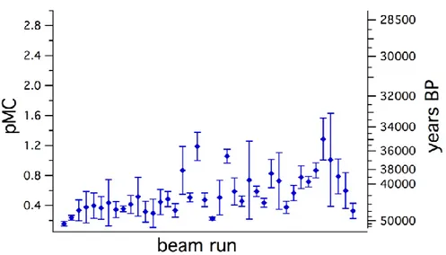
The new line was designed because, during the years, a slight increase of the pMC value in blank samples was noticed, as it is shown in Figure 3.2 where the average blank values measured during five years are reported. As it is said in chapter 2, the blank samples are characterized by a 14C concentration nominally equal to zero or, at least, well below the sensitivity limit of AMS; hence, these samples give us the possibility to verify whether contaminations have been introduced during sample preparation and AMS measurement, estimating the background contribution (due to both sample processing and measurement in the accelerator). In fact, an increase of the pMC value measured in blanks corresponds to a decrease of the sensitivity achievable in the AMS measurements, putting a limit on the oldest sample that can be dated.
Fig 3.2 Average blank values measured since 2004 until 2009. Each point represents the average calculated
over the several blanks measured in a same beam run; the quoted error corresponds to the maximum deviation. On the left y-axis the radiocarbon concentration, expressed in pMC, is reported; on the right y-axis the corresponding radiocarbon age expressed in years BP is shown.
The new graphitization line was thus thought in order to: improve the vacuum level in the line;
reduce the effect of contamination possibly correlated to the graphitization process and to the deterioration of some mechanical components of the line.
The line (see Figure 3.3) was designed keeping the structure of the old graphitization line, adding some improvements:
installation of a new Swagelok® three-way valve at the outlet of the elemental analyser (EA), in order to easily switch the gas flowing from the EA either into the line or into
atmosphere;
substitution of the old LN2 trap with a new spiral trap arranged in the horizontal plane
in order to provide a homogeneous cooling in liquid nitrogen;
addition of a new connection to transfer the CO2 obtained from samples that are not
combusted in the elemental analyzer6;
capability of installing up to eight graphitization reactors in order to have the possibility to prepare up to eight samples in parallel.
The schematic layout of the new graphitization line is presented in Figure 3.4.
Fig. 3.3 Schematic layout of the new graphitization line.
Talking about how to operate on the line, the gaseous mixture of CO2 and helium coming out
from the elemental analyzer7 is transferred to the graphitization line thanks to the new 3-way switching valve. The valve is switched to the line just in the moment when the CO2 is flowing, i.e.
when the correspondent peak is visible in the chromatogram. In the graphitization line, the gases
6 For instance, carbonates (e.g. foraminifera and shells) can be either combusted using the EA or can undergo a chemical reaction (3CaCO3 + 2 H3PO4 Ca3(PO4)2 + 3CO2 + 3H2O), which takes place in an independent dedicated preparation line.
7 It is worth to remember that helium is used in the EA as carrier to transport the gases through the combustion and gaschromatographic columns and the gas detector.
Pumping system Sample in H2 Pumping system LN2 trap HV gauge LV gauge A C B Exhaust to air Elemental analyzer Swagelok® Ultra-Torr
Swagelok® Switching (3-Way) Valve
A B C
are first collected in the freezing trap (LN2 in Figure 3.3). Since helium does not condense at the
LN2 temperature, it can be removed by the pumping system8 while carbon dioxide is kept frozen
in the trap. Afterwards, when the helium is completely removed, the spiral is heated and CO2 can
be transferred to the quartz reactor where graphitization takes place. The quartz tube for the reaction has been already filled with iron powder that acts as catalyst in the graphitization (see equation 2.3). A double quantity of hydrogen with respect to the CO2 is also added in the reactor
in order to convert the CO2 into elemental carbon, i.e. graphite (see the reaction described in
paragraph 2.1.2, equation (2.3)). Since the reaction takes place at 600°C, the tube filled with iron is inserted in an oven. At the same time, the water, secondary product of the reaction, is trapped in order to prevent the reverse reaction to start. To this purpose, the other quartz tube of the reactor acts as a cool finger inserted in a Peltier cooling device (reaching a temperature of about -20°C). After about two hours and a half, the reaction is complete and the graphite sample is obtained. In Figure 3.4, the typical pressure trend of the graphitization reaction is shown.
0 200 400 600 800 1000 1200 0 20 40 60 80 100 120 140 160 180 time (min) p re s s u re ( m b a r)
Fig 3.4 Typical pressure trend of the graphitisation reaction.
3.1.1 Accuracy tests performed using the new graphitization line
In order to test the new graphitization line, several samples were prepared and measured, in particular blanks and standard reference materials with certified 14C concentration, i.e.:
8 The dry pumping system is based on a diaphragm pump and a turbo molecular pump; the choice of these dry pumps was done in order to reduce possible contamination effects due to the presence of oil (for example the oil of a diffusion preliminary pumps).
IAEA C7 (certified radiocarbon concentration 49.53±0.12 pMC), an Oxalic Acid standard reference material supplied by the International Atomic Energy Agency;
VIRI D (certified radiocarbon age 2836±4 years BP): seeds from an archaeological excavation in Israel, dispatched to the laboratory within the Fifth International Radiocarbon Intercomparison (VIRI) campaign [Sco2007];
VIRI S (certified radiocarbon concentration 109.96±0.04 pMC): barley mashes collected in a Scottish whiskey factory, dispatched to the laboratory within the Fifth International Radiocarbon Intercomparison (VIRI) campaign [Sco2010].
In Figures 3.5-8 the measured radiocarbon concentrations or radiocarbon age of these materials are reported.
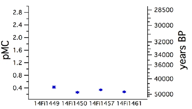
Fig. 3.5 Radiocarbon concentrations measured in blank samples expressed in percent of Modern Carbon; on
the right y axis, the corresponding radiocarbon ages in years BP are also reported.
48.00 48.50 49.00 49.50 50.00 50.50 51.00
14Fi1453 14Fi1455 14Fi1458 14Fi1468 14Fi1463
p
M
C
Fig. 3.6 Radiocarbon concentrations expressed in percent of Modern Carbon measured in standard IAEA C7
samples. The certified value (49.53±0.12 pMC) is represented with the dotted line. The experimental uncertainty on each sample concentration is quoted as 1 sigma.
2600 2700 2800 2900 3000 3100 3200 14Fi1462 14Fi1467 ye a rs B P
Fig. 3.7 Conventional radiocarbon ages expressed in years Before Present measured in VIRI D samples. The
certified value (2836±4 years BP) is represented with the dotted line. The experimental uncertainty on each sample age is quoted as 1 sigma.
105 107 109 111 113 115 14Fi1464 14Fi1466 p M C
Fig. 3.8 Radiocarbon concentrations expressed in percent of Modern Carbon measured in VIRI S samples.
The certified value (109.96±0.04 pMC) is represented with the dotted line. The experimental uncertainty on each sample concentration is quoted as 1 sigma.
The radiocarbon concentrations measured in blank samples are satisfactory and of the same order of magnitude of the typical concentrations measured in the first years of operation of the AMS facility at LABEC.
Concerning the standard materials, the data are consistent with the certified values. Only the 14C concentration measured in samples 14Fi1462 and 14Fi1464 is slightly different with respect to the certified value; however, the two results are within 2 sigma confidence levels and thus can be accepted.
3.2 Upgrade of the AMS beam line
In chapter 2, the AMS beam line installed at the Tandem accelerator of LABEC was described; in particular, the rare isotope detection system based on the employment of an ionization chamber was presented.
Despite all the filters present on the AMS beam line and as a consequence of recombination or charge-exchange processes, some particles that simulate the same combination of energy, mass and charge of 14C atoms might arrive on the detector. Considering the low energy resolution of the ionization chamber (about 70 keV) [Laz2007], identifying the residual atomic/molecular interferences with this system is not possible.
In the framework of an experiment funded by INFN (Istituto Nazionale di Fisica Nucleare), the final part of the AMS beam line has completely been re-designed: new detection system have been installed in order to improve the capability of discrimination, thus paving the way also to the measurements of rare isotopes other than 14C. The upgrade has affected the line at the exit of the high energy electrostatic analyzer. The new channel is equipped with:
a new silicon particle detector;
a multiwire proportional chamber used as a beam profile monitor (BPM) for very low intensity ion beams (few tens of counts per second) [Tac2010];
a time of flight system (TOF) with start and stop signals provided by modules based on micro-channel plates.
In Figure 3.9, a schematic drawing of the new channel is shown.
Fig. 3.9 Schematic drawing of the new AMS beam line installed at the exit of the electrostatic analyzer on
the high energy side.
As a consequence of the addition of new elements, the AMS beam line was extended; in particular the rare isotope detector, now the silicon one, has been moved ahead of about 200 cm. In principle, this might have introduced some difficulties in the beam transport, since the only focusing element is represented by the electrostatic quadrupole doublets already installed at the exit of the electrostatic analyser, just before the new valve (see the blue valve in Figure 3.9).
In this section, only the upgrade concerning the new installed detector is described, being a part of this PhD work. The new detector is a Hamamatsu Silicon PIN photodiode S3590-09, having an active area of 100 mm2 and a thickness of 300 μm. In Figure 3.10, the silicon detector and the retractable arm on which it is mounted are shown.
Silicon detector Faraday cup BPM Pumping system Pumping system TOF start TOF stop beam
Fig 3.10 The new silicon detector (indicated by the black arrow) mounted on a retractable arm.
In Figure 3.11 a comparison between a spectrum acquired with the “old” ionization chamber and the new silicon detector is reported.
Fig 3.11 Beam energy spectra acquired with the ionization chamber and the silicon detector.
The comparison between the two detectors shows a remarkable improvement of the energy resolution by using the silicon photodiode. This means that it would be possible to identify the presence of possible particles having a slightly different energy with respect to the atoms of interest.
low counting rate (see paragraph 2.7); however, it is well known that the exposure of this detectors to charged particle causes a significant deterioration in their performance. Serious changes of the energy resolution typically take place after the detector has been irradiated with about 108 ions/cm2 [Kno1979]. To estimate the degree of deterioration of the new installed detector after two years of operation, we can do a simple calculation considering that, since its installation at the beginning of 2010, approximately 600 samples have been measured. Assuming for each modern sample:
a counting rate of about 15 counts/s·cm2;
a measuring time of 60 min (which is needed to acquire a reasonable number of total counts to reach the desired level of precision);
it is possible to calculate a total flux of ~3·107 ions/cm2, still below the certified critical limit. It is worth to remember that this estimate represents an upper limit because most of the measured samples are characterized by a lower counting rate with respect to the modern samples (as one could expect, the oldest is the sample, the lower is the counting rate).
3.2.1 Accuracy tests of the upgraded AMS beam line
The upgraded AMS beam line was tested measuring the radiocarbon concentration in standard materials of certified 14C abundance. The analyzed standard materials were IAEA C7, VIRI D, VIRI S (see paragraph 3.1.1) and:
VIRI O (certified radiocarbon concentration 98.46±0.04 pMC), cellulose collected from Cambridge corresponding to 60 rings from a plateau period, dispatched to the laboratory within the Fifth International Radiocarbon Intercomparison (VIRI) campaign [Sco2010].

![Fig 1.3 Portion of IntCal09, the atmospheric calibration curve [Rei2009]. On the y axis the radiocarbon age,](https://thumb-eu.123doks.com/thumbv2/123dokorg/4731819.46122/14.892.148.733.113.406/fig-portion-intcal-atmospheric-calibration-curve-rei-radiocarbon.webp)
![Fig 1.8 Portion of the table of nuclides showing carbon isotopes and their neighbours [wAt2000]](https://thumb-eu.123doks.com/thumbv2/123dokorg/4731819.46122/18.892.186.657.569.832/fig-portion-table-nuclides-showing-carbon-isotopes-neighbours.webp)