Water and Sediment Output Evaluation Using Cellular Automata on Alpine Catchment: Soana, Italy - Test Case

(1)

IOP Conference Series: Earth and Environmental Science

PAPER • OPEN ACCESS

Water and Sediment Output Evaluation Using

Cellular Automata on Alpine Catchment: Soana,

Italy - Test Case

To cite this article: Antonio Pasculli et al 2017 IOP Conf. Ser.: Earth Environ. Sci. 95 022031

View the article online for updates and enhancements.

Water and Sediment Output Evaluation Using Cellular

Automata on Alpine Catchment: Soana, Italy - Test Case

Antonio Pasculli1_{, Chiara Audisio}1,2_{, Nicola Sciarra}1

1_{Department of Engineering and Geology (INGEO), University of Chieti-Pescara, Via}

dei Vestini 31, Chieti, Italy

2 _{Città Metropolitana di Torino, Italy}

antonio.pasculli@unich.it

Abstract. In the alpine contest, the estimation of the rainfall (inflow) and the discharge

(outflow) data are very important in order to, at least, analyse historical time series at catchment scale; determine the hydrological maximum and minimum estimate flood and drought frequency. Hydrological researches become a precious source of information for various human activities, in particular for land use management and planning. Many rainfall-runoff models have been proposed to reflect steady, gradually-varied flow condition inside a catchment. In these last years, the application of Reduced Complexity Models (RCM) has been representing an excellent alternative resource for evaluating the hydrological response of catchments, within a period of time up to decades. Hence, this paper is aimed at the discussion of the application of the research code CAESAR, based on cellular automaton (CA) approach, in order to evaluate the water and the sediment outputs from an alpine catchment (Soana, Italy), selected as test case. The comparison between the predicted numerical results, developed through parametric analysis, and the available measured data are discussed. Finally, the analysis of a numerical estimate of the sediment budget over ten years is presented. The necessity of a fast, but reliable numerical support when the measured data are not so easily accessible, as in Alpine catchments, is highlighted.

1. Introduction

The rainfall and hydrometric data are often available with great difficulty or, even if the measurement instruments are present in the catchment, their position is not always appropriate. The application of rainfall-runoff model, which represents the major components of the water system, is an effective tool, commonly employed in this kind of studies. The use of simple models, usually, can solve just only few aspects of some problems. On the other hand, the category known as 'complex conceptual models' assumed that most of their parameters could be defined from the physiographic characteristics of the basins. In this field, commonly utilized approaches are based on the balance equations of physics, pursued by the CFD (Computational Fluid Dynamic) and the RCM. Nearly, all CFD rely on solving Navier-Stokes flow equations [1], supplemented by experimental laws that define the parameters related to the mass transport of material, the rate of erosion (for instance: [2]), etc. Besides the most common 'grid based methods', another category of approaches was proposed: the mesh-less solution of the differential equation. Among others, SPH (Smoothed Particle Hydrodynamics) appears to be promising ([3], [4], among many others). On the other hand, the RCM, to which Cellular Automata (CA, [5]) approach belongs, now, represents an important alternative to the CFD. CAESAR, a CA

(3)

2 1234567890

research code, is a 2D flow and sediment model [6]. It was conceived to be applied in order to predict morphological changes, within large area and over relevant time scale (climate evolution as well), both at reach ([7]; [8]) and at catchment scale ([9]). More details could be found in [10]. The analyses in this paper were carried out with the CAESAR version 6.1f and 6.2m, with two purposes: a further testing of the capability of a CA model to predict discharges on a catchment's scale, not properly gauged, through the comparison between measured and predicted data and, after the identification of the most appropriate input parameters values, an estimate of the sediment budget along a period of ten years. The method is applied on an Alpine catchment, Soana (Western Italy), selected as a test case.

2. Selected test case

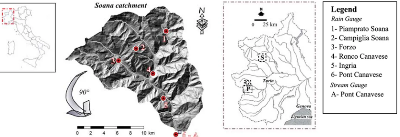
The Soana catchment, is located in the North Western Sector of the Italian Alps (Graian Alps), in Piedmont region bordering to the North with Aosta Valley (Figure 1). The available acquired time series regard only a relatively short period (less than ten years).

Several hydroelectric plants, affecting the hydrology management of the territory, are located within the basin. For the measured discharge, the Pont Canavese time series (2002-2012) (see Figure 1 for the instruments location) was selected. Slide activation usually follows extreme rainfall or flood. Intense rainfall, frequent in summer, can trigger shallow slides, hyperconcentrated flow or debris flows. Furthermore, frequent wetting and drying phenomena, lowering soil mechanical strength (in particular for pyroclastic soils, in the South of Italy ([11]; [12]), may trigger possible landslides occurrences and, accordingly, morphological variation of the territory.

3. Data inputs

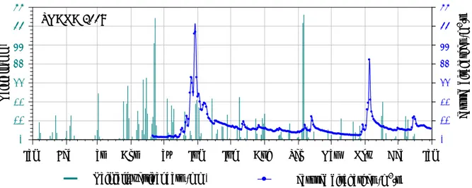
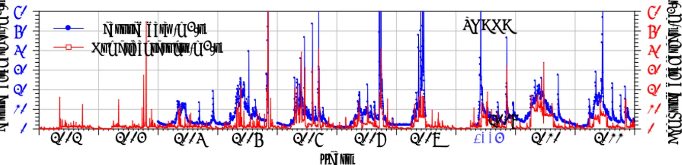
The topographic data was derived from a Digital Elevation Model. In order to meet the CAESAR's requirements, we used a 50 x 50 m grid DEM (Regione Piemonte), obtaining 154,049 cells. Exploiting available datasets, the localization of bedrock and, further, the cells in which erosion is avoided were acquired. Then, the obtained vectorial dataset was converted in a raster (named 'land use') based on the bedrock presence or absence (considering also the vegetation and type of deposits). The Piamprato's rainfall gauge and Pont Canavese stream gauge for the measured discharges (respectively '1' and 'A' in Figure 1) were selected as representative for the analysis discussed in this paper. In Figure 2 the rainfall and the discharges measured during the calibration year 2009 are reported. Finally, the granulometric data were derived from available bibliography.

(4)

1234567890

Jan Feb Mar Apr May Jun Jul Aug Sep Oct Nov Dec Jan

0 11 22 33 44 55 66 77 0 11 22 33 44 55 66 77 Measured discharges (m3/s) SOANA 2009 R ain fa ll ( m m ) Measu red d is ch arges ( m 3 /s )

Rainfall, vertical bars (mm)

Figure 2. Daily rainfall and measured discharges within a selected year (2009) 4. Methods

Oreskes et al. [13] specified and discussed the appropriate strategies with which to evaluate numerical models in the Earth Sciences. At least three possible approaches were proposed: (1) the sensitivity analysis of the results changing the numerical values of some selected parameters and grid structure; (2) the comparison of the model prediction with measured data; (3) the comparison between the results coming from the selected model and alternative approaches. Thus, in order to calibrate the catchment modality implemented in CAESAR, we performed a comparison between the predicted and the measured discharge based on a sort of sensitivity analysis (first Oreskes's strategy). Because of the high demand of CPU computation time, the sensitivity analysis was performed within a period of just one selected year (2009). The selection of the rainfall, exploited as the main CAESAR's inputs, and the stream gauges were performed on empirical considerations. However, the measured discharges may be influenced by many other sources. By consequence, in order to test how much the selected rainfall time series could affect the comparisons among simulations and the available data regarding discharges, we conducted the main part of test changing the input precipitation (total or half) and

m-coeff parameter, strictly related to the vegetation cover, the catchment storage capacity and

transmissivity. The m-coeff is derived, essentially, from the effect of the flood hydrograph on the recession limb. Then, in some simulations we tested a few additional parameters of the model: 1) the 'flow distribution cell', that indicates the number of cells involved in the discharge distribution; 2) the 'max erodible limit', that specifies the maximum amount of material that can be eroded or deposited within a cell; 3) the 'active layer' that represents thickness of a single active layer and 4) the 'initial

number of scan', referring to the number of scans that are required to establish the zone or buffer

around the channel where the CAESAR algorithm focused the numerical elaborations. Totally, 18 simulation tests were carried out. Then we performed the simulations, the most significant of which with the values of some important input parameters are reported in Table 1. As 'rainfall' we indicated the fraction (50% or 100%), utilized as input, of the actual measured rainfall.

(5)

4 1234567890

Table 1. Soana catchment simulations set up.

Simulation rainfall m-coeff flow distrib. cell max erod. limit active layer initial # of scan

S2 total 0.001 4 0.02 0.2 10 S3 total 0.002 4 0.02 0.2 10 S4 total 0.003 4 0.02 0.2 10 S5 total 0.005 4 0.02 0.2 10 S6 0.5 0.001 4 0.02 0.2 10 S7 0.5 0.002 4 0.02 0.2 10 S8 0.5 0.003 4 0.02 0.2 10 S9 0.5 0.005 4 0.02 0.2 10 S11 total 0.002 4 0.04 0.2 20 S12 total 0.002 4 0.08 0.4 20 S13 total 0.002 4 0.04 0.5 20 S14 total 0.002 4 0.05 0.2 20

A direct comparison between computed and measured discharges over a period of 10 years, (following the second Oreskes's strategy) were carried out. Moreover, the inventory of the sediments and their distribution within the water flow (turbulence, deposition, saltation and so on) was particularly hard to acquire directly in situ. Thus, in order to test the reasonability of the computed estimates of the sediments inventory, at least respect to alternative approaches (the third Oreskes's strategy), we compared the CAESAR's numerical outputs, already calibrated by sensitivity analyses, to the results obtained through two commonly worldwide used erosion models.

5. Results

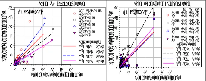
Then, in Figure 3a the calculated discharges of selected simulations, in particular with different

m-coeff (MC), described in Table 1, were linearly compared to one another, while in Figure 3b, max-erod.-limit (ER) and active-layer (AL) were changed, setting m-coeff (MC) = 0.002. Each simulation

introduced above generated a time series of the discharges, consisting of 365 values, one for each day of the selected year (2009). In order to describe the resulting numerical ensemble by a global point of view, a suitable tool that could be used is the analysis of some of their statistical moments, reported in Table 2. Therefore, a second kind of calibration was performed. In Figure 4 the comparison among the resulting CAESAR's computed discharges, referred to just one year (2009) (12 cyan filled circles) and the statistical parameters resulting from the ensembles of the measured discharges data related to a period ranging from 2003 to 2010 (8 black crosses) are displayed.

Soana m-coeff comparison

Discharge (total rainfall, m3/s)

0 10 20 30 40 50 60

D

ischarge (half rai

nfall , m 3 /s) 0 3 6 9 12 15 18 S6(MC=0.001) vs S2(0.001) S7(0.002) vs S3(0.002) S8(0.003) vs S4(0.003) S9(0.005) vs S5(0.005) Linear regression R2 = 0.501 S6-S2 R2 = 0.745 S7-S3 R2 = 0.816 S8-S4 R2 = 0.614 S9-S5 (a)year 2009

Soana sediment and cell comparison

Discharge (total rainfall, m3/s)

0 10 20 30 40 50 60 D is ch ar ge (t ot al r ai nf al l, m 3 /s ) 0 5 10 15 20 25 30 R2 = 0.714 S11-S3 R2 = 0.876 S12-S3 R2 = 0.681 S13-S3 R2 = 0.724 S14-S3 Linear regression MC ER AL S11 vs 0.002 0.04 0.2 S31vs 0.002 0.02 0.2 S12 vs 0.002 0.08 0.4 S32vs 0.002 0.02 0.2 S13 vs 0.002 0.04 0.5 S33vs 0.002 0.02 0.2 S14 vs 0.002 0.05 0.2 S34vs 0.002 0.02 0.2 (b) year 2009

Figure 3. Comparison among different simulations of the predicted discharges; MC: m-coeff; ER:

(6)

1234567890

Red circles around a black cross, indicate the yearly averages of the selected statistical parameters of the measured discharges ensemble related to the year 2009. Beside each red circles, the labels of the simulations whose statistical parameters are more close than others to the values of the measured ensemble, are indicated.

Table 2. Statistical parameters

Name Formula Notes

Sample moment of r-th order r

m

=



  n 1 i r i μ x n 1 ) ˆ

( Statistical central moment about the mean μˆ

(information about distribution's shape) Standard Deviation 2 1 2

m

σ

_ˆ

_

/ ₌







n 1 i 2 i

μˆ

)

x

(

n

1

Provides a measure of the _{data spread around the}

sample mean Skewness 3 3 1

σ

m

γ

ˆ



= 3 n 1 i 2 i n 1 i 3 i

x

μ

n

1 μ

x

n

1 











_













_



 

)

ˆ

(

)

ˆ

(

Asymmetry of the data

around the median.; a

negative skew (left) has fewer low values and a positive skew (right) has fewer large values. Kurtosis 4 4

σ

m

k

ˆ

ˆ 

=

_n

1 x

μ

_n

1 x

μ

3

4 n 1 i 2 i n 1 i 4 i















_













_

_

_

 

)

ˆ

(

)

ˆ

(

A high kurtosis value

indicates that the distribution has a sharp peak with long and fat tails.

Figure 4. Comparison between statistical moments of the computed discharges data obtained by all

the simulations performed during the year 2009 and the statistical moments of the measured discharges obtained from 2003 to 2010.

Thus, from Figure 3 and 4, after some attempts, comparing computed data to measured discharges over a period of 10 years, the parameters reported in Table 3 were selected.

Table 3. Input parameters for sediment evaluation at catchment scale used for the ten years’

simulation.

Rainfall m coeff max-erodible- limit active layer initial # scan flow

distribution total 0.005 0.02 0.2 20 4 Variance 0 50 100 150 200 Conf idence interval 0 50 100 150 200 c) S3 year 2009 S2 Standard deviation 0 4 8 12 16 Max imu m d isc ha rge ( m 3 /s) 0 50 100 150 200 a) year 2009 S3 S5 S2 Kurtosis 0 75 150 225 300 Ske w nes s 0 5 10 15 20 computed data measured data b) year 2009 S9

Soana (reference year: 2009)

computed data: Table 1 measured data: years 2003-2010

(7)

6 1234567890

Accordingly, the best obtained results are reported in Figure 5, regarding the partially complete time series of measured and computed discharges from 2002 to 2011. In particular, the comparison related to the selected year 2009, used as a calibration year, is reported in Figure 6.

0 10 20 30 40 50 60 0 10 20 30 40 50 60 Measured data (m3/s) Numerical results (m3/s) SOANA 2009 2009 2008 2007 2006 2005 2004 2003 2002 2010 2011 years Me asu red discharges ( m 3/s) C om put ed d is cha rges (m 3/s )

Figure 5. Computed vs measured discharges comparison, within ten years, without missing data.

0 10 20 30 40 50 60 70 0 10 20 30 40 50 60 70 Measured discharges (m3/s) Computed discharges (m3/s) Rainfall (mm) vertical bars SOANA 2009 M

easured and com

puted di scharges (m 3/s ) Rain fal l ( m m )

Jan Feb Mar Apr May Jun Jul Aug Sep Oct Nov Dec Jan

Figure 6. Computed, measured and rainfall comparison, during the year 2009.

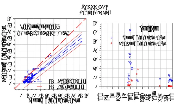
Moreover, in Figure 7, the direct comparison between the computed and the available measured discharges during the selected year 2009, is displayed. The final plot (left part) was obtained after the outliers exclusion by inspection of the confidence bands, resulting from the first comparison, based on raw data. The linear regression index R2_{indicates how much we can 'align' data along a straight line.}

Also, it shows how much data has been scattered around a trend. On the other hand, the angular coefficient of the regression line indicates how much the two sets of data are correctly correlated with each other. The maximum correlation value is obviously m = 1, which corresponds to 45 degrees (red dashed line). In Figure 7 the angular coefficient of the linear regression is about 76% of the perfect correlation between measured and computed discharges with the exclusion of the outliers values. Moreover, it is interesting to note (right part of the Figure 7) that the outliers are clustered at the half and at the end period of the year.

6. Sediment estimate

Employing the parameters values obtained by the previous calibration and comparison analyses (Table 3, Figures. 5, 6), a simulations of the total sediments produced in the selected year 2009 was performed. Then, considering the common method for soil erosion evaluation such as Rusle [14] and Gavrilovic [15], we can estimate that, potentially, the Soana's catchment can produce annually millions of cubic meters of sediment, as also CEASAR has evidenced. Comparing the three different methods (Table 4), the annual soil erosion rate resulting from Caesar's calculations underestimate the values obtained by Rusle and Gavrilovic approaches. However, due to the complexity of the attempt, this results could be considered quite satisfactory. (for detailed description of the parameters R, K, C, P, X, Y, G, introduced in Table 3, see Rusle [14]).

(8)

1234567890

Measured discharges (m3_/s) 0 5 10 15 20 25 30 35 40 45 50 C om puted discharge s (m 3/s) 0 5 10 15 20 25 30 35 40 45 50 76 0 R 75 1 x 79 0 y_ _. _ _ _. _; 2 _ _. SOANA 2009 (16 Jun - 12 Dec) 0 10 20 30 40 50 60 70 Measured discharges (m3_/s) Computed discharges (m3_/s)

Jan Feb _Mar Apr _May Jun Jul _Aug Sep Oc

t No v De c Jan

Linear regression :

_outliers

95% Confidence Band 95% Prediction Band

Figure 7. Computed discharges compared directly to measured discharges; left, comparison without

outliers; right, the excluded outliers.

Table 4. Comparison of soil erosion between CAESAR’s predicted value and the values derived by

the two equation of Rusle and Gavrilovic (in bold). Data are in m/year.

RUSLE GAVRILOVIC CAESAR

R K C P LS X Y G

SOANA 1360 0.036 0.14 1 30 0.31 1.51 0.25

0.014 0.014 0.006

All these analyses allowed the selection of the most suitable numerical values of the input parameters in order to perform a further simulation aimed at evaluating ten years sediment production. The results are reported in Figure 8.

Days 500 1000 1500 2000 2500 3000 3500 4000 Cu mu lative s edim

ent output pre

diction (m 3 ) 0.0 5.0e+5 1.0e+6 1.5e+6 2.0e+6 2.5e+6 Cumulative sediment Sigmoidal regression: R2_=0.961

(9)

8 1234567890

The following sigmoidal regression expression could be used as a predictive tool to estimate the quantity of sediment produced by the selected basin over time.

]

695 .

162 /

)

871 .

622 ]

[

exp(

1 [

025 .

2 ]

[

3 ) (

Mm





t

day



S

_S

(1)

7. Discussion

The Figure 3a indicates the first notable aspect: the predicted discharge, calculated by CAESAR using the total rainfall as input (abscissa), usually triples or sometimes quadruples the predicted discharges using the half rainfall as input (ordinate). This occurrence is independent of the value assigned to the

m-coeff. R2_{is always less than 0.82. However, in many simulations, considering the half rainfall as}

input, the highest predicted discharges were always underestimated; on the other hand, the total rainfall as input tends to slightly overestimate the predicted discharge. Therefore, the use of the total rainfall needs to be correctly evaluated with the m-coeff. From Figure 3b, it is clear the influence of the 'max erodible limit' on the predicted discharge. In Figure 3b, S3 is progressively compared to other simulations characterized by increased values of the 'max erodible limit' and or different 'active layer' values (S11, S12, S13, S14, Table 1). From simulations not reported, also the 'initial number of scan', which determines how many scans the model performs before the next water-sediment passage, is an important input parameter. Furthermore, higher is the 'initial number of scan', higher is the iterations number and, accordingly, longer is the run time. The comparison between predicted and measured discharge was carried out through the use of statistics and taking in account the whole series of measured data. Soana catchment reveals an incoherent comparison related to the high discharge data (Figures. 5, 6 and 7). The same trend is evident comparing the confidence interval and the variance of data (Figure 4c). Then, the kurtosis and skewness of the discharge distributions were reported. The generally positive and high value of skewness, both in measured and predicted data, confirm the large difference between the mean and the median of data. The kurtosis values are very high indicating the sharp peak both of measured and predicted data. From Figure 7 clearly emerges the need to consider the melting of the snow, but also the hydrological capacity of the basin, possible

anthropomorphic

factors and others causes to be explored in much details

. It is also important to consider the correlation that may exist between the selected rainfall gauges and the flow rate gauges selected for comparison, but not analyzed in this paper.

8. Conclusions

The comparison among several simulation tests and the comparison between the discharge predicted by the CA model and the measured data at the selected stream gauge are illustrated and discussed. In addition, after this comparison, the sediment outputs were estimated over a period of ten years and the soil erosion rates are evaluated and compared to other common methods of evaluation. The sediment discharge appears to be largely dependent on the rainfall (flood) magnitude, but the sensitivity analysis demonstrated also the influence of the vegetation cover in the catchment. The sediment model, if compared to common methods of analysis of soil erosion, predicts reliable value of soil erosion rates and volumes, after appropriate calibration. An additional advantage of CAESAR utilization is the computational speed and power, compared to CFD approaches. With opportune calibration and validation, CAESAR can be used as a tool to predict several geomorphological and hydrological evolution or sediment flux from a catchment in order to anticipate possible future change, in particular, in this contest of climatic variation and alpine catchment evolution. Moreover, it is worth noting that since the sediment output of a catchment is an important input for evaluating the morphological evolution of a river embedded in the selected basin, the outcomes obtained by the application of CAESAR in catchment modality, in particular the resulting sediment output would be the input for the CAESAR model at reach scale modality.

(10)

1234567890

References

[1] Pasculli, A., 2008. CFD-FEM 2D Modeling of a local water flow. Some numerical results.

Alpine and Mediterranean Quaternary (ex: “Il Quaternario, Italian Journal of Quaternary Sciences”), vol. 21 (1B), pp. 215–228. ISSN: 22797327; SCOPUS id: 2-s2.0-84983037047.

[2] Pasculli, A., Sciarra, N., 2006. A probalistic approach to determine the local erosion of a watery debris flow. 11th International Congress for Mathematical Geology: Quantitative Geology

from Multiple Sources, IAMG 2006, Liege, Belgium. ISBN: 978-296006440-7; SCOPUS id:

2-s2.0-84902449614.

[3] Minatti, L., Pasculli, A., 2010. Dam break Smoothed Particle Hydrodynamic modeling based on Riemann solvers. WIT Transactions on Engineering Sciences, vol. 69 pp.145-156. ISSN: 1743-3533; ISBN: 978-184564476-5; doi: 10.2495/AFM100131; SCOPUS id: 2-s2.0-78449235684.

[4] Pasculli, A., Minatti, L., Audisio, C., Sciarra, N., 2014. Insights on the application of some current SPH approaches for the study of muddy debris flow: numerical and experimental comparison. WIT Transactions on Engineering Sciences, vol. 82, pp. 3-14. ISSN: 17433533; ISBN: 978-1-84564-790-2; doi: 10.2495/AFM140011; SCOPUS id: 2-s2.0-84907611231.

[5] Wolfram, S., 1983. Statistical Mechanics of Cellular Automata. Reviews of Modern Physics, vol. 55, pp. 601-644.

[6] http://www.coulthard.org.uk/CAESAR.html

[7] Pasculli, A., Audisio, C., 2015. Cellular automata modelling of fluvial evolution: real and parametric numerical results comparison along River Pellice (NW Italy). Environmental

Modelling and Assessment, vol. 20 (5), pp. 425-441. ISSN: 14202026; doi:

10.1007/s10666-015-9444-8; WOS: 000360554900002; SCOPUS id: 2-s2.0-84940588890. [8] Audisio, C, Pasculli, A, Sciarra, N., 2015. Conceptual and numerical models applied on the

River Pellice (North Western Italy). In: Engineering Geology for Society and Territory. Vol. 3. Springer International Publishing Switzerland, pp. 327–330; ISBN: 978-3-319-09053-5. doi: 10.1007/978-3-319-09054-68; WOS: 000358990300068; SCOPUS id: 2-s2.0-84944586202.

[9] Pasculli, A., Audisio, C., Sciarra, N., 2015. Application of CAESAR for catchment and river evolution. Rend Online Soc Geol It, vol. 35, pp. 224-227. ISSN: 20358008; doi: 10.3301/ROL.2015.106; WOS:000373173500058; SCOPUS id: 2-s2.0-84930707096. [10] Coulthard, T.J., Macklin, M.G., Kirkby, M.J., 2002. A cellular model of Holocene upland river

basin and alluvial fan formation. Earth Surf Processes and Landf, vol. 27, pp. 269–288. [11] Esposito, L., Esposito, A.W., Pasculli, A., Sciarra, N., 2013. Particular features of the physical

and mechanical characteristics of certain Phlegraean pyroclastic soils. CATENA, vol. 104, pp. 186-194. ISSN: 03418162; doi: 10.1016/j.catena.2012.11.009; WOS: 000315556600019; SCOPUS id: 2-s2.0-84873130083.

[12] Pasculli, A., Sciarra, N., Esposito, L., Esposito, A.W., 2017. Effects of wetting and drying cycles on mechanical properties of pyroclastic soils. CATENA, vol. 156, pp. 113-123. ISSN: 03418162 doi: 10.1016/j.catena.2017.04.004; SCOPUS id: 2-s2.0-85017109027. [13] Oreskes, N., Shrader-Frechette, K., Belitz, K., 1994. Verification, Validation, and Confirmation

of Numerical Models in the Earth Science. Science, vol. 263, pp. 641-646. [14] Rusle, 2015-http://esdac.jrc.ec.europa.eu/themes/rusle2015.

[15] Gavrilovic, S., 1959. Méthode de la classification des bassins torrentiels et équations nouvelles pour le calcul des hautes eaux et du débit solide. Vadopriveda, Belgrado.

Water and Sediment Output Evaluation Using Cellular Automata on Alpine Catchment: Soana, Italy - Test Case

IOP Conference Series: Earth and Environmental Science