Multivariate Analysis Applications in X-ray Diffraction

Crystals 2021, 11, 12. https://doi.org/10.3390/cryst11010012 www.mdpi.com/journal/crystals Review

Multivariate Analysis Applications in X-ray Diffraction

1 _{Dipartimento di Ingegneria Elettrica e dell’Informazione, Politecnico di Bari, via Orabona 4,}

70125 Bari, Italy; pietro.guccione@gmail.com

2 _{Dipartimento di Scienze e Innovazione Tecnologica, Università del Piemonte Orientale, viale T. Michel 11,}

15121 Alessandria, Italy; mattia.lopresti@uniupo.it (M.L.); marco.milanesio@uniupo.it (M.M.)

3 _{Institute of Crystallography, CNR, via Amendola, 122/o, 70126 Bari, Italy}

* Correspondence: rocco.caliandro@ic.cnr.it; Tel.: +39-080-592-9150

Abstract: Multivariate analysis (MA) is becoming a fundamental tool for processing in an efficient

way the large amount of data collected in X-ray diffraction experiments. Multi-wedge data collections can increase the data quality in case of tiny protein crystals; in situ or operando setups allow investigating changes on powder samples occurring during repeated fast measurements; pump and probe experiments at X-ray free-electron laser (XFEL) sources supply structural characterization of fast photo-excitation processes. In all these cases, MA can facilitate the extraction of relevant information hidden in data, disclosing the possibility of automatic data processing even in absence of a priori structural knowledge. MA methods recently used in the field of X-ray diffraction are here reviewed and described, giving hints about theoretical background and possible applications. The use of MA in the framework of the modulated enhanced diffraction technique is described in detail.

Keywords: multivariate analysis; chemometrics; principal component analysis; partial least square;

X-ray powder diffraction; X-ray single crystal diffraction

1. Introduction

Multivariate analysis (MA) consists of the application of a set of mathematical tools to problems involving more than one variable in large datasets, often combining data from different sources to find hidden structures. MA provides decomposition in simpler components and makes predictions based on models or recovers signals buried in data noise.

Analysis of dependency of data in more dimensions (or variables) can be derived from the former work of Gauss on linear regression (LR) and successively generalized to more than one predictor by Yule and Pearson, who reformulated the linear relation between explanatory and response variables in a joint context [1,2].

The need to solve problems of data decomposition into simpler components and simplify the multivariate regression using few, representative explanatory variables brought towards the advent of the principal component analysis (PCA) by Pearson and, later, by Hotelling [3,4] in the first years of the 20th century. Since then, PCA has been considered a great step towards data analysis exploration because the idea of data decomposition into its principal axes (analogies with mechanics and physics were noted by the authors) allows the data to be explained into a new multidimensional space, where directions are orthogonal to each other (i.e., the new variables are uncorrelated) and each successive direction is decreasing in importance and, therefore, in explained variance. This paved the way to the concept of dimensionality reduction [5] that is crucially important in many research areas such as chemometrics.

Chemometrics involves primarily the use of statistical tools in analytical chemistry [6] and, for this reason, it is as aged as MA. It is also for this reason that the two disciplines started to talk since the late 1960s, initially concerning the use of factor analysis (FA) in

Citation: Guccione, P.; Lopresti, M.;

Milanesio, M.; Caliandro, R. Multivariate Analysis Applications in X-ray diffraction. 2021, 11, 12. https://doi.org/10.3390/cryst11010012 Received: 21 November 2020 Accepted: 21 December 2020 Published: 25 December 2020

Publisher’s Note: MDPI stays

neutral with regard to jurisdictional claims in published maps and institutional affiliations.

Copyright: © 2020 by the author.

Licensee MDPI, Basel, Switzerland. This article is an open access article distributed under the terms and conditions of the Creative Commons Attribution (CC BY) license (http://creativecommons.org/licenses /by/4.0/).

chromatography [7]. FA is a different way to see the same problem faced by PCA, as in FA data are explained by hidden variables (latent variables or factors) by using different conditions for factor extraction [8], while in PCA components are extracted by using the variance maximization as unique criterion. Since then, chemometrics and MA have contaminated each other drawing both advantages [9].

Multivariate curve resolution (MCR) [10] is a recent development consisting in the separation of multicomponent systems and able to provide a scientifically meaningful bilinear model of pure contributions from the information of the mixed measurements. Another data modeling tool is the partial least square (PLS) [11], a regression method that avoids the bad conditioning intrinsic of LR by projecting the explanatory variables onto a new space where the variables are uncorrelated each other, but maximally correlated with the dependent variable. PLS has been successfully applied in problems such as quantitative structure-activity vs. quantitative structure-property of dataset of peptides [12] or in the analysis of relation of crystallite shapes in synthesis of super-structures of CaCO3 through a hydrogel membrane platform [13].

Moreover, classification methods have been adopted in chemometrics since the beginning, mainly for pattern recognition, i.e., classification of objects in groups according to structures dictated by variables. Discriminant analysis (DA), PLS-DA [14], support vector machines (SM) [15] have been used for problems such as classification of food quality or adulteration on the basis of sensitive crystallization [16], toxicity of sediment samples [17] or in classification of biomarkers [18], gene data expression or proteomics [19] just to mention few examples.

MA has been also used to improve the signal-to-noise ratio in measurements. Methods such as phase sensitive detection (PSD) have been developed and implemented for technical applications as in the lock-in amplifier, which amplifies only signals in phase with an internal reference signal. PSD has found a large applications in chemometrics connected to excitation enhanced spectroscopy, where it has been used to highlight excitation-response correlations in chemical systems [20]. Summarizing, although widely used in analytical chemistry, MA is less diffused in materials science and certainly under-exploited in crystallography, where much wider applications are forecast in the next decade.

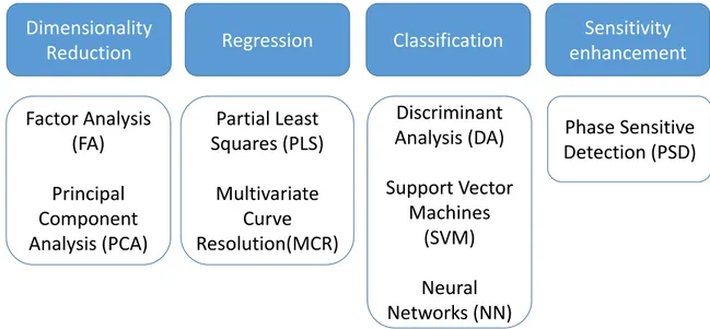
The main multivariate methods, grouped according to their main field of application, are outlined in Figure 1. In the following, they are critically compared each other, with particular attention on the specificity of chemometric problems and applications to crystallography. In detail, the bad conditioning due to the high dimensionality and the concept of overfitting is analyzed and the needs and advantages in reducing the problem of dimensionality are discussed (Section 2.1); then, similar methods are put in comparison in the successive subsections: PCA vs. FA vs. MCR for dimensionality reduction (Section 2.2), with particular attention to X-ray diffraction applications. In Section 3 we describe a new technique, called modulated enhanced diffraction (MED), which allows the extraction of signals from single components from complex crystal systems monitored by X-ray diffraction experiment, showing the convergence of PSD (a Fourier deconvolution approach) with standard and constrained (OCCR) PCA approaches. PCA, MCR and FA applications to the investigation of powder samples and single-crystal samples by X-ray diffraction are reviewed in sections 4 and 5, respectively. In detail, Section 4 is devoted to the main applications to kinetic (4.1) and quantitative analysis (4.2). Examples of these two main applications are given to highlight the wide potentialities of MA-based approaches. Section 5 describes the results and perspectives in single crystal diffraction, in details in solving the phase problem (Section 5.1) merging datasets (Section 5.2) and crystal monitoring (Section 5.3), exploiting the capability of MA methods in general and PCA in particular to highlight dynamic phenomena.

Figure 1. Schematic view showing main multivariate methods grouped according to their field of application.

2. Multivariate Methods

2.1. High Dimension and Overfitting

MA provides answers for prediction, data structure, parameter estimations. In facing these problems, we can think at data collected from experiments as objects of an unknown manifold in a hyperspace of many dimensions [21]. In the context of X-ray diffraction, experimental data are constituted by diffraction patterns in case of single crystals or dif-fraction profiles in case of powder samples. Difdif-fraction patterns, after indexing, are con-stituted by a set of reflections, each identified by three integers (the Miller indices) and an intensity value, while diffraction profiles are formed by 2ϑ values as independent variable and intensity values as dependent variable. The data dimensionality depends on the num-ber of reflections or on the numnum-ber of 2ϑ values included in the dataset. Thus, high-reso-lution data contain more information about the crystal system under investigation, but have also higher dimensionality.

In this powerful and suggestive representation, prediction, parameter estimation, finding latent variables or structure in data (such as classify or clustering) are all different aspects of the same problem: model the data, i.e., retrieve the characteristics of such a complex hypersurface plunged within a hyperspace, by using just a sampling of it. Some-times, few other properties can be added to aid the construction of the model, such as the smoothness of the manifold (the hypersurface) that represents the physical model under-lying the data. Mathematically speaking, this means that the hypersurface is locally ho-meomorphic to a Euclidean space and can be useful to make derivatives, finding local minimum in optimization and so on.

In MA, it is common to consider balanced a problem in which the number of variables involved is significantly fewer than the number of samples. In such situations, the sam-pling of the manifold is adequate and statistical methods to infer its model are robust enough to make predictions, structuring and so on. Unfortunately, in chemometrics it is common to face problems in which the number of dimensions is much higher than the number of samples. Some notable examples involve diffraction/scattering profiles, but other cases can be found in bioinformatics, in study for gene expression in DNA microar-ray [22,23]. Getting high resolution data is considered a good result in Crystallography. However, this implies a larger number of variables describing a dataset: (more reflections in case of single-crystal data or higher 2ϑ values in case of powder data). Consequently, it makes more complicated the application of MA.

When the dimensionality increases, the volume of the space increases so fast that the available data become sparse on the hypersurface, making it difficult to infer any trend in

Dimensionality

Reduction

Regression

Classification

Sensitivity

enhancement

Factor Analysis

(FA)

Principal

Component

Analysis (PCA)

Partial Least

Squares (PLS)

Multivariate

Curve

Resolution(MCR)

Discriminant

Analysis (DA)

Support Vector

Machines

(SVM)

Neural

Networks (NN)

Phase Sensitive

Detection (PSD)

data. In other words, the sparsity becomes rapidly problematic for any method that re-quires statistical significance. In principle, to keep the same amount of information (i.e., to support the results) the number of samples should grow exponentially with the dimen-sion of the problem.

A drawback of having a so much high number of dimensions is the risk of overfitting. Overfitting is an excessive adjustment of the model to data. When a model is built, it must account for an adequate number of parameters in order to explain the data. However, this should not be done too precisely, so to keep the right amount of generality in explaining another set of data that would be extracted from the same experiment or population. This feature is commonly known as model’s robustness. Adapting a model to the data too tightly introduces spurious parameters that explain the residuals and natural oscillations of data commonly imputed to noise. This known problem was named by Bellman the “curse of dimensionality” [5], but it has other names (e.g., the Hughes phenomenon in classification). A way to partially mitigate such impairment is to reduce the number of dimensions of the problem, giving up to some characteristic of the data structure.

The dimensionality reduction can be performed by following two different strategies: selection of variables or transformation of variables. In the literature, the methods are known as feature selection and feature extraction [24].

Formally, if we model each variate of the problem as a random variable Xi, the

selec-tion of variables is the process of selecting a subset of relevant variables to be used for model construction. This selection requires some optimality criterion, i.e., it is performed according to an agreed method of judgement. Problems to which feature selection meth-ods can be applied are the ones where one of the variables, Y, has the role of ‘response’, i.e., it has some degree of dependency from the remaining variables. The optimality crite-rion is then based on the maximization of a performance figure, achieved by combining a subset of variables and the response. In this way, each variable is judged by its level of relevance or redundancy compared to the others, to explain Y. An example of such a fig-ure of performance is the information gain (IG) [25], which resorts from the concept of entropy, developed in the information theory. IG is a measure of the gain in information achieved by the response variable (Y) when a new variable (Xi) is introduced into the

measure. Formally:

𝐼𝐺(𝑌, 𝑋 ) = 𝐻(𝑌) − 𝐻(𝑌|𝑋 ) (1)

being H() the entropy of the random variable. High value of IG means that the second term 𝐻(𝑌|𝑋 ) is little compared to the first one, 𝐻(𝑌), i.e., that when the new variable 𝑋 is introduced, it explains well the response 𝑌 and the corresponding entropy becomes low. The highest values of IG are used to decide which variables are relevant for the re-sponse prediction. If the rere-sponse variable is discrete (i.e., used to classify), another suc-cessful method is Relief [26], which is based on the idea that the ranking of features can be decided on the basis of weights coming from the measured distance of each sample (of a given class) from nearby samples of different classes and the distance of the same sample measured from nearby samples of the same class. The highest weights provide the most relevant features, able to make the best prediction of the response.

Such methods have found application in the analysis of DNA microarray data, where the number of variables (up to tenths of thousands) is much higher than the number of samples (few hundreds), to select the genes responsible for the expression of some rele-vant characteristic, as in the presence of a genetic disease [27]. Another relerele-vant applica-tion can be found in proteomics [28], where the number of different proteins under study or retrieved in a particular experimental environment is not comparable with the bigger number of protein features, so that reduction of data through the identification of the rel-evant feature becomes essential to discern the most important ones [29].

Feature extraction methods, instead, are based on the idea of transforming the varia-bles set into another set of reduced size. Using a simple and general mathematical formu-lation, we have:

𝑌 , … , 𝑌 = 𝑓( 𝑋 , … , 𝑋 ), 𝑚 ≪ 𝑛 (2) with the output set [Y1,…,Ym] a completely different set of features from the input

[X1,…,Xn], but achieved from them. Common feature-extraction methods are based on

lin-ear transformation, i.e.,

𝒀 = 𝐴𝑿, 𝑚 ≪ 𝑛 (3)

where the variables are transformed losing their original meaning to get new characteris-tics that may reveal some hidden structure in data.

Among these methods, PCA is based on the transformation in a space where varia-bles are all uncorrelated each other and sorted by decreasing variance. Independent Com-ponent Analysis (ICA), instead, transforms variables in a space where they are all inde-pendent each other and maximally not-Gaussian, apart for one, which represents the un-explained part of the model, typically noise. Other methods, such as MCR, solve the prob-lem by applying more complicated conditions such as the positivity of the values in the new set of variables or similar, so that the physical meaning of the data is still preserved. A critical review of dimensionality reduction feature extraction methods is in Section 2.2. PCA and MCR have an important application in solving mixing problems or in de-composing powder diffraction profiles of mixtures in pure-phase components. In such decomposition, the first principal components (or contributions, in MCR terminology) usually include the pure-phase profiles or have a high correlation with these.

2.2. Dimensionality Reduction Methods

In Section 2.1, the importance of applying dimensionality reduction to simplify the problem view and reveal underlying model within data was underlined. One of the most common method to make dimensionality reduction is principal component analysis.

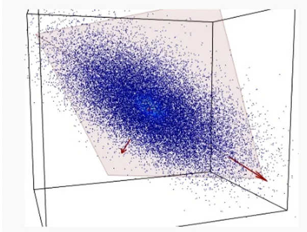
PCA is a method to decompose a data matrix finding new variables orthogonal each other (i.e., uncorrelated), while preserving the maximum variance (see Figure 2). These new uncorrelated variables are named principal components (PCs).

Figure 2. A set of data (blue dots) of three variables is represented into a 3D space. Data are mostly

spread on the orange plane, with little departure from it. Principle component analysis (PCA) identifies the plane and the directions of maximum variability of data within it.

PCA is then an orthogonal linear transformation that transforms data from the cur-rent space of variables to a new space of the same dimension (in this sense, no reduction of dimension is applied), but so that the greatest variance lies on the first coordinate, the second greatest variance on the second coordinate and so on. From a mathematical view-point, said X the dataset, of size N × P (N being the number of samples, P that of the vari-ates), PCA decomposes it so that

𝑿 = 𝑻𝑾′ (4) with 𝑻 (of size N × P) the matrix of the principal components (called also scores), which are the transformed variable values corresponding to each sample and with 𝑾 (of size P × P) the matrix of the loadings, corresponding to the weights by which each original vari-able must be multiplied to get the component scores. The matrix 𝑾 is composed by or-thogonal columns that are the eigenvectors of the diagonalization [30] of the sample co-variance matrix of 𝑿:

𝑿′𝑿 = 𝑾′𝚲𝑾 (5)

In Equation (5), 𝚲 is a diagonal matrix containing the eigenvalues of the sample co-variance matrix of 𝑿, i.e., 𝑿′𝑿. Since a coco-variance matrix is always semi-definite positive, the eigenvalues are all real and positive or null and correspond to the explained variance of each principal component. The main idea behind PCA is that in making such decom-position, often occurs that not all the directions are equally important. Rather, the number of directions preserving most of the explained variance (i.e., energy) of the data are few, often the first 1–3 principal components (PC). Dimensionality reduction is then a lossy process, in which data are reconstructed by an acceptable approximation that uses just the first few principal components, while the remaining are neglected:

𝑿 ≈ 𝑻(𝟏:𝒔)𝑾′(𝟏:𝒔) (6)

With 𝒔 the retained components (i.e., the first s columns of both the matrices) and 𝒔 ≪ 𝑷.

Diagonalization of the covariance matrix of data is the heart of PCA and it is achieved by resorting to singular value decomposition (SVD), a basic methodology in linear alge-bra. SVD should not be confused with PCA, the main difference being the meaning given to the results. In SVD the input matrix is decomposed into the product a left matrix of eigenvectors 𝑼, a diagonal matrix of eigenvalues 𝚲 and a right matrix of eigenvectors 𝑽, reading the decomposition from left to right:

𝒀 = 𝑼𝚲𝑽′ (7)

SVD may provide decomposition also of rectangular matrices. PCA, instead, uses SVD for diagonalization of the data covariance matrix 𝑿′𝑿, which is square and semi-definite positive. Therefore, left and right eigenvector matrices are the same, and the di-agonal matrix is square and with real and positive value included. The choice of the most important eigenvalues allows the choice of the components to retain, a step that is missing from SVD meaning.

Factor analysis is a method based on the same concept of PCA: a dataset is explained by a linear combination of hidden factors, which are uncorrelated each other, apart for a residual error:

𝑿 = 𝒍𝟏𝑭𝟏+ ⋯ 𝒍𝒏𝑭𝒏+ 𝜺 (8)

FA is a more elaborated version of PCA in which factors are supposed (usually) to be known in number and, although orthogonal each other (as in PCA), they can be achieved adopting external conditions to the problem. A common way to extract factors in FA is by using a depletion method in which the dataset 𝑿 is subjected to an iterative extraction of factors that can be analyzed time by time: 𝑿(𝒌)= 𝑿(𝒌 𝟏)− 𝒍𝐤𝑭𝐤. In FA, there is the clear

intent to find physical causes of the model in the linear combination. For this reason, their number is fixed and independency of the factors with the residual 𝜺 is imposed too. It can be considered, then, a supervised deconvolution of original dataset in which inde-pendent and fixed number of factors must be found. PCA, instead, explores uncorrelated directions without any intent of fixing the number of the most important ones.

FA has been applied as an alternative to PCA in reducing the number of parameters and various structural descriptors for different molecules in chromatographic datasets

[31]. Moreover, developments of the original concepts have been achieved by introducing a certain degree of complexity such as the shifting of factors [32] (factors can have a certain degree of misalignment in the time direction, such as in the time profile for X-ray powder diffraction data) or the shifting and warping (i.e., a time stretching) [33].

Exploring more complete linear decomposition methods, MCR [8] has found some success as a family of methods that solve the mixture analysis problem, i.e., the problem of finding the pure-phase contribution and the amount of mixing into a data matrix in-cluding only the mixed measurements. A typical paradigm for MCR, as well as for PCA, is represented by spectroscopic or X-ray diffraction data. In this context, each row of the data matrix represents a different profile, where the columns are the spectral channels or diffraction/scattering angles, and the different rows are the different spectra or profiles recorded during the change of an external condition during time.

In MCR analysis, the dataset is described as the contribution coming from reference components (or profiles), weighted by coefficients that vary their action through time:

𝑿𝒊≈ 𝒄𝒊𝑺′𝒊 (9)

With 𝒄𝒊 the vector of weights (the profile of change of the i-th profile through time)

and 𝑺𝒊 the pure-phase i-th reference profile. The approximation sign is since MCR leaves

some degree of uncertainty in the model. In a compact form we have:

𝑿 = 𝑪𝑺 + 𝑬 (10)

MCR shares the same mathematical model of PCA, apart for the inclusion of a resid-ual contribution 𝑬 that represents the part of the model we give up explaining. The algo-rithm that solves the mixture problem in the MCR approach, however, is quite different from the one used in PCA. While PCA is mainly based on the singular value decomposi-tion (i.e., basically the diagonalizadecomposi-tion of its sample covariance matrix), MCR is based on the alternating least square (ALS) algorithm, an iterative method that tries to solve condi-tioned minimum square problems of the form:

𝑪, 𝑺 = 𝑎𝑟𝑔𝑚𝑖𝑛𝑪,𝑺 𝒙, − 𝒄 𝒔′ + 𝜆 ‖𝒄𝒊‖ + 𝒔 ,

(11) The previous problem is a least square problem with a regularization term properly weighted by a Lagrange parameter 𝝀. The regularization term, quite common in optimi-zation problems, is used to drive the solution so that it owns some characteristics. The 𝑳𝟐

-norm of the columns of 𝑺 or 𝑪, as reported in the Equation (11), is used to minimize the energy of the residual and it is the most common way to solve ALS. However, other reg-ularizations exist, such as 𝑳𝟏-norm to get more sparse solutions [34] or imposing

positiv-ity of the elements of 𝑺 and 𝑪. Usually, the solution to Equation (11) is provided by iter-ative methods, where initial guesses of the decomposition matrices 𝑺 or 𝑪 are substi-tuted iteratively by alternating the solution of the least-square problem and the applica-tion of the constraints. In MCR, the condiapplica-tion of positivity of elements in both 𝑺 or 𝑪 is fundamental to give physical meaning to matrices that represent profile intensity and mixing amounts, respectively.

The MCR solution does not provide the direction of maximum variability as PCA. PCA makes no assumption on data; the principal components and particularly the first one, try to catch the main trend of variability through time (or samples). MCR imposes external conditions (such as the positivity), it is more powerful, but also more computa-tionally intensive. Moreover, for quite complicated data structures, such as the ones mod-eling the evolution of crystalline phases through time [35,36], it could be quite difficult to impose constraints into the regularization term, making the iterative search unstable if not properly set [37,38]. Another important difference between MCR and PCA is in the model selection: in MCR the number of latent variables (i.e., the number of profiles in which decomposition must be done) must be known and set in advance; in PCA, instead, while

there are some criterion of selection of the number of significative PC such as the Mali-nowski indicator function (MIF) [39,40] or the average eigenvalue criterion (AEC) [41,42], it can also be inferred by simply looking at the trend of the eigenvalues, which is typical of an unsupervised approach. The most informative principal components are the ones with highest values.

For simple mathematical models, it will be shown in practical cases taken from X-ray diffraction that PCA is able to optimally identify the components without external con-straints. In other cases, when the model is more complicated, we successfully experi-mented a variation of PCA called orthogonal constrained component rotation (OCCR) [43]. In OCCR, a post-processing is applied after PCA aimed at revealing the directions of the first few principal components that can satisfy external constraints, given by the model. The components, this way, are no longer required to keep the orthogonality. OCCR is then an optimization method in which the selected principal components of the model are let free to explore their subspace until a condition imposed by the data model is optimized. OCCR has been shown to give results that are better than traditional PCA, even when PCA produces already satisfactory results. A practical example (see Section 3) is the decomposition of the MED dataset in pure-phase profiles, where PCA scores, pro-portional to profiles, may be related each other with specific equations.

Smoothed principal component analysis or (SPCA) is a modification of common PCA suited for complex data matrices coming from single or multi-technique approaches where the time is a variable, in which sampling is a continuous, such as in situ experiment or kinetic studies. The ratio behind the algorithm proposed by Silvermann [44] is that data without noise should be smooth. For this reason, in continuous data, such as profiles or time-resolved data, the eigenvector that describes the variance of data should be also smooth [45]. Within these assumptions, a function called “roughness function” is inserted within the PCA algorithm for searching the eigenvectors along the directions of maximum variance. The aim of the procedure is reducing the noise in the data by promoting the smoothness between the eigenvectors and discouraging more discrete and less continuous data. SPCA had been successfully applied to crystallographic data in solution-mediated kinetic studies of polymorphs, such as L-glutamic acid from α to β form by Dharmayat et al. [46] or p-Aminobenzoic acid from α to β form by Turner and colleagues [47].

3. Modulated Enhanced Diffraction

The Modulated Enhanced Diffraction (MED) technique has been conceived to achieve chemical selectivity in X-ray diffraction. Series of measurements from in situ or operando X-ray diffraction experiments, where the sample is subjected to a varying exter-nal stimulus, can be processed by MA to extract information about active atoms, i.e., at-oms of the sample responding to the applied stimulus. This approach has the great ad-vantage of not requiring preliminary structural information, so it can be applied to com-plex systems, such as composite materials, quasi-amorphous samples, multi-component solid-state processes, with the aim to characterize the (simpler) sub-structure comprising active atoms. The main steps involved in a MED experiment are sketched in Figure 3. During data collection of X-ray diffraction data, the crystal sample is perturbed by apply-ing an external stimulus that can be controlled in its shape and duration. The stimulus determines a variation of structural parameters of the crystallized molecule and/or of the crystal lattice itself. These changes represent the response of the crystal, which is usually unknown. Repeated X-ray diffraction measurements allow to collect diffraction patterns at different times, thus sampling the effect of the external perturbation. In principle, the set of collected diffraction patterns can be used to detect the diffraction response to the stimulus. Offline data analysis based on MA methods must be applied to implement the deconvolution step, i.e., to process time-dependent diffraction intensities Ih measured for

each reflection h to recover the time evolution of the parameters for each atom j of the crystal structure, such as occupancy (nj), atomic scattering factor (fj) and atomic position

the detected variable, depend on the square of the structure factors Fh, embedding the

actual response of the system.

Figure 3. Main steps involved in a MED experiment. A perturbation is applied in a controlled way on a crystal sample,

which responds by changing the crystal structural parameters in unknown way. Repeated X-ray diffraction measurements allow detecting the diffraction response, which can be properly analyzed through an offline process called deconvolution, to determine the variations in main structural parameters.

Applications of MED are twofold: on one hand, the active atoms sub-structure can be recovered, so disclosing information at atomic scale about the part of the system chang-ing with the stimulus, on the other hand the kinetic of changes occurrchang-ing in the sample can be immediately captured, even ignoring the nature of such changes.

To achieve both these goals, MA tools have been developed and successfully applied to crystallographic case studies. These methods, which will be surveyed in the next para-graph, implement the so-called data deconvolution, i.e., they allow extracting a single MED profile out of the data matrix comprising the set of measurements.

Deconvolution Methods

The first deconvolution method applied to MED technique was sensitive phase detec-tion (SPD). SPD is a MA approach widely applied since decades to spectroscopic data (mod-ulation enhanced spectroscopy—MES), which can be applied to systems linearly respond-ing to periodic stimuli. SPD projects the system response from time domain to phase domain by using a reference periodic -typically sinusoidal- signal, through the following Equation:

𝒑(𝒙, 𝝋) =𝟐 𝑵 𝒚𝒊(𝒙)𝒔𝒊𝒏 𝟐𝑲𝝅 𝑵 𝒊 + 𝝋 𝑵 𝒊 𝟎 (12) where φ is the SPD phase angle, yi(x) are the n measurements collected at the time i, and k is the order of the demodulation. The variable x can be the angular variable 2ϑ in case

of X-ray powder diffraction measurements or the reflection h in case of single-crystal dif-fraction data. Equation (12) represents a demodulation in the frequency space of the system response, collected in the time space. Demodulation at k = 1, i.e., at the lower frequency of the reference signal, allows the extraction of kinetic features, involving both active and silent atoms; demodulation at k = 2, i.e., at double the lower frequency of the reference signal, allow to single out contribution from only active atoms. This was demonstrated in [35] and comes from the unique property of X-ray diffraction that the measured intensities Ih depends on the square of the structure factors Fh. A pictorial way to deduce this property

is given in Figure 4: silent and active atoms respond in a different way to the external stimulus applied to the crystal. This can be parameterized by assigning different time de-pendences to their structure factors, respectively FS and FA. For sake of simplicity, we can

assume that silent atoms do not respond at all to the stimulus, thus FS remain constant

during the experiment, while active atoms respond elastically, thus FA has the same time

dependence of that of the stimulus applied (supposed sinusoidal in Figure 4). In these hypotheses, the diffraction response can be divided in three terms, the first being constant, the second having the same time dependence of the stimulus, the third having a doubled frequency with respect to that of the stimulus and representing the contribution of active atoms only. PSD performed incredibly well for the first case study considered, where the adsorption of Xe atoms in an MFI zeolite was monitored in situ by X-ray diffraction, by using pressure or temperature variations as external stimulus [48,49]. However, it was immediately clear that this approach had very limited applications, since very few sys-tems, only in particular conditions, have a linear response -mandatory to apply PSD for the demodulation- to periodic stimuli, and it is easier to apply non-periodic stimuli.

Figure 4. Pictorial demonstration of the possibility to extract information of active atoms only in a MED experiment. The

crystal system is divided in silent (S) and active (A) atoms, depending on how they respond to an external stimulus ap-plied. The diffraction response measured on the X-ray detector can be divided in two contributions from S and A atoms. This give rise to three terms, the first being constant in time, the second having the same time-dependence of the stimulus, the third varying with double the frequency of the stimulus and representing the contribution of active atoms only.

A more general approach would allow coping with periodic stimuli and non-linear system responses. To this aim, PCA was applied to MED data, with the underlying idea that in simple cases, the first principal component (PC1) should capture changes due to active and silent atoms, the second principal component (PC2) should instead capture changes due to active atoms only. In fact, if the time-dependence of the contribution from active atoms can be separated, i.e., 𝑭𝑨(𝒕) = 𝑭𝑨∗ 𝒈(𝒕), then the MED demodulation shown

in Figure 4 can be written in a matrix form: 𝑰𝒉= (𝟏 𝒈(𝒕) 𝒈(𝒕)𝟐) ∗

𝑭𝑺𝟐

𝟐𝑭𝑨𝑭𝑺𝐜𝐨𝐬(𝝋𝑨− 𝝋𝑺)

𝑭𝑨𝟐

(13) By comparing Equation (13) with Equation (12) it can be inferred that PCA scores should capture the time-dependence of the stimulus, while PCA loadings should capture the dependence from the 2ϑ or h variable of the diffraction pattern. In particular, we ex-pect two significant principal component, the first having 𝑻𝟏= 𝒈(𝒕) and 𝑾𝟏=

𝟐𝑭𝑨𝑭𝑺𝐜𝐨𝐬(𝝋𝑨− 𝝋𝑺), the second having 𝑻𝟐= 𝒈(𝒕)𝟐 and 𝑾𝟐= 𝑭𝑨𝟐. Notably, constant

terms are excluded by PCA processing, since in PCA it is assumed zero-mean of the data

-1,0 -0,5 0,0 0,5 1,0 Time

S

A

Detector

F

+

F

2

F

_{+ 2}

_F

F

cos(φ

-φ

) +

F

Crystal

Sinusoidal stimulus

Same frequency of stimulus

Doubled frequency

Atoms A respond elastically

matrix columns. An example of deconvolution carried out by PCA, which is more properly referred to as decomposition of the system response, is shown in Figure 5, consid-ering in situ X-ray powder diffraction data. The PC1 scores reproduce the time depend-ence of the applied stimulus, whereas PC2 scores have a doubled frequency. PC1 loadings have positive and negative peaks, depending on the values of the phase angles 𝝋𝑨 and

𝝋𝑺, while PC2 loadings have only positive peaks, representing the diffraction pattern from

active atoms only.

Figure 5. Example of PCA decomposition applied to in situ X-ray powder diffraction data. Scores

(a) and loadings (b) of the first principal component (PC1); scores (c) and loadings (d) of the second principal component (PC2). A sinusoidal stimulus was applied during the in situ experiment.

In this framework, a rationale can be figured out, where the PC1 term is like the k = 1 PSD term and the PC2 term is like the k = 2 PSD term. This correspondence is strict for systems responding linearly to periodic stimuli, while for more general systems PCA is the only way to perform decomposition. This new approach was successfully applied to different case studies [50,51] outperforming the PSD method.

Another important advancement in MED development was to introduce adapted variants of existing MA methods. In fact, PCA decomposition cannot be accomplished as outlined above for complex systems, where several parts (sub-structures) vary with dif-ferent time trends, each of them captured by specific components. A signature for failure of the standard PCA approach is a high number of principal components describing non-negligible data variability, and failure to satisfy two conditions for PC1 and PC2, descend-ing from the above-mentioned squared dependence of measured intensity from structure factors. In the standard PCA case, PC2 loadings, which describe the data variability across reflections (or 2ϑ axis in case of powder samples), are expected to be positive, given the proportionality with squared structure factors of only active atoms. Moreover, PC1 and PC2 scores, which describe the data variability across measurements, are expected to fol-low the relation:

𝑻𝟐= (𝑻𝟏)𝟐 (14)

as changes for active atoms vary with a frequency doubled with respect to that of the stimulus. A MA approach adapted to MED analysis has been developed, where constraints on PC2 loadings and on PC1/PC2 scores according to Equation (14) are included in the PCA decomposition. This gave rise to a new MA method, called orthogonal constrained com-ponent rotation (OCCR), which aims at finding the best rotations of the principal compo-nents determined by PCA, driven by figure of merits based on the two MED constraints. The OCCR approach allows overcoming the main limitation of PCA, i.e., to blind

search-ing components that are mutually orthogonal. It has been successfully applied to charac-terize water-splitting processes catalyzed by spinel compounds [43] or to locate Xe atoms in the MFI zeolite to an unprecedented precision [50].

A further advancement in the route of routinely applying PCA to MED was done in [51,52], where the output of PCA was analytically derived, and expected contribution to scores and loadings to specific changes in crystallographic parameters have been listed. This would make easier the interpretation of the results of PCA decomposition.

4. Applications in Powder X-ray Diffraction

X-ray powder diffraction (XRPD) offers the advantage of very fast measurements, as many crystals are in diffracting orientation under the X-ray beam at the same time. A complete diffraction pattern at reasonable statistics can be acquired in seconds, even with lab equipment and such high measurement rates enable the possibility to perform in situ experiments, where repeated measurements are made on the same sample, while varying some external variable, the most simple one being time [53]. On the other hand, the con-temporary diffraction from many crystals makes it difficult to retrieve structural infor-mation about the average crystal structure by using phasing methods. In this context, MA has great potential, since it allows extracting relevant information from raw data, which could be used to carry out the crystal structure determination process on subset of atoms, or to characterize the system under study without any prior structural knowledge. Some specific applications of MA on powder X-ray diffraction are reviewed in the following sections. The two main fields of applications are the extraction of dynamic data (Section 4.1) in a temporal gradient and qualitative and quantitative analysis (Section 4.2) in pres-ence of concentration gradients.

4.1. Kinetic Studies by Single or Multi-Probe Experiments

The advent of MA has also revolutionized kinetic studies based on in situ powder X-ray diffraction measurements. Several works have used MA to extract efficiently the reac-tion coordinate from raw measurements [54–56]. Moreover, in a recent study of solid-state reactions of organic compounds, the classical approach of fitting the reaction coordinate by several kinetic models has been replaced by a new approach, which embeds kinetic models within the PCA decomposition [57,58]. The discrimination of the best kinetic model is enhanced by the fact that it produces both the best estimate of the reaction coor-dinate and the best agreement with the theoretical model. MCR-ALS is another decompo-sition method that had been employed in the last few years in several kinetic studies on chemical reactions [59–61].

MA is even more powerful when applied to datasets acquired in multi-technique ex-periments, where X-ray diffraction is complemented by one or more other techniques. The MA approach allows, in these cases, to extract at best the information by the different instruments, probing complementary features. In fact, the complete characterization of an evolving system is nowadays achieved by complex in situ experiments that adopt multi-probe measurements, where X-ray measurements are combined with spectroscopic probes, such as Raman FT-IR or UV-vis spectroscopy. In this context, covariance maps have been used to identify correlated features present in diffraction and spectroscopic profiles. Examples include investigations of temperature-induced phase changes in spin crossover materials by XRPD/Raman [36] perovskites by combining XRPD and pair dis-tribution function (PDF) measurements [62], characterization of hybrid composite mate-rial known as Maya Blue performed by XRPD/UV-Vis [63] and metabolite-crystalline phase correlation in wine leaves by XRPD coupled with mass spectrometry and nuclear magnetic resonance [64].

To highlight the potentialities of the application of PCA to unravel dynamics from in situ X-ray diffraction studies, a recently published case study [52] is briefly described. In this paper, the sedimentation of barium sulfate additive inside an oligomeric mixture was studied during polymerization by repeated XRPD measurements with a scan rate of

1°/min. The kinetic behavior of the sedimentation process was investigated by processing the high number (150) of XRPD patterns with PCA, without using any prior structural knowledge. The trend in data can hardly be observed by visual inspection of the data matrix (Figure 6a), as the peak intensity does not change with a clear trend and their po-sitions drift to lower 2ϑ values during the data collection. PCA processes the whole data matrix in seconds, obtaining a PC that explains the 89% of the system’s variance (Figure 6b). The loadings associated to this PC resemble the first derivative of an XRPD profile (Figure 6c), suggesting that this PC captured the changes in data due to barite peak shift toward lower 2ϑ values. In fact, PCA, looking for the maximum variance in the data, ba-sically extract from the data and highlight the variations of the signal through time. PCA scores, which characterize in the time domain the variations in data highlighted by load-ings, indicate a decreasing trend (Figure 6d). In fact, the peak shift is strongly evident at the beginning of the reaction, with an asymptotic trend at the end of the experiment. Scores in Figure 6d can thus be interpreted as the reaction coordinate of the sedimentation process. In ref. [52], the comparison of PCA scores with the zero-error obtained by Rietveld refinement confirmed that the dynamic trend extracted by PCA is consistent with that derived from the traditional approach. However, the time for data processing (few seconds with MA, few hours with Rietveld Refinement) makes PCA a very useful com-plementary tool to extract dynamic and kinetic data while executing the experiment, to check data quality and monitor the results without a priori information.

Figure 6. In situ analysis of sedimentation data for barite additive in an oligomeric mixture during gelation time; 150

measurements were collected during the experiment, covering the angular range of the three more intense peaks of barium sulfate XRPD profile; (a) Analyzed data matrix; (b) scree plot; (c) loadings plot; (d) score plot.

4.2. Qualitative and Quantitative Studies

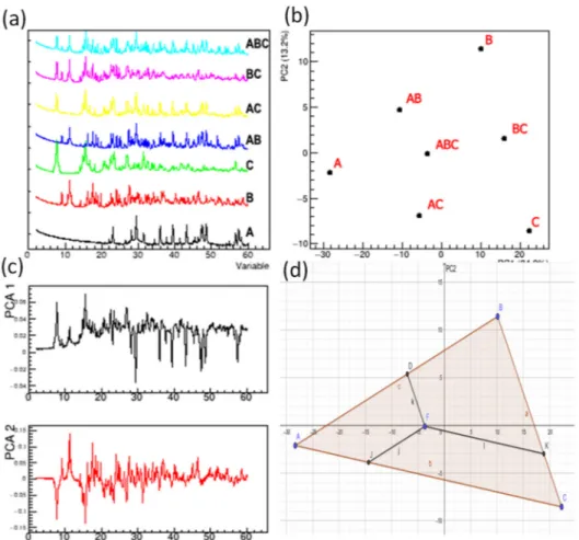
Having prompt hints about main trends in data is beneficial in many applications and can facilitate subsequent structural analysis. Qualitative and/or quantitative analysis on sets from X-ray powder diffraction profiles can be achieved by both FA [65,66] and PCA, particularly from the score values of the main components. This approach is com-mon in the -omics sciences in the analytical chemistry field. Euclidean distances in PC score plots can be calculated to obtain also a semi-quantitative estimation between groups or clusters [67,68]. In fact, the arrangement of representative points in the scores plot can be used to guess the composition of the mixture. An example of application of this ap-proach is given in Figure 7. Figure 7a reports the original X-ray diffraction data collected on pure phases (A, B, C), the binary mixtures (AB, BC, AC) 50:50 weight and ternary mix-ture ABC prepared by properly mixing calcium carbonate (A), acetylsalicylic acid (B) and sodium citrate (C). PCA analysis was carried out and the corresponding PC scores (Figure 7b) and loadings (Figure 7c) are reported. It is evident that the PCA scores are sensible to %weight of the samples since they form a triangle with the monophasic datasets (A, B, C) at the vertices, the binary mixtures (AB, BC, AC) in the middle of the edges and the ternary mixture ABC in its center. All the possible mixtures are within the triangle, in the typical representation of a ternary mixture experimental domain. PCA recognizes the single-phase contributions by the PC loadings, containing the XRPD pattern features, high-lighted in Figure 7c. PC1 loadings have positive peaks corresponding to phases B and C, and negative ones to phase A. PC2 loadings show positive peaks corresponding to phase B and negative ones to phase C, while phase A has a very moderate negative contribution, being located close to 0 along the PC2 axis in Figure 7b.

Figure 7. Original data (a), PC scores (b), PC loading (c) and calculation of Euclidean distances from PC scores (d) from

X-ray powder diffraction data by ternary mixtures. Data points A, B, and C correspond to powder diffraction profiles from monophasic mixtures, data points AB, AC and BC to binary mixtures and ABC to a mixture containing an equal amount of the three crystal phases.

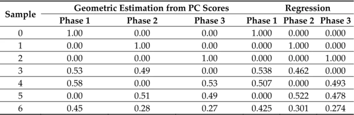
PCA scores in Figure 7b can be exploited to perform a semi-quantitative analysis, since the above described dependence of the topology of data points in the scores plot is related to the composition. The procedure is easy for binary and ternary mixtures where a 2D plot (Figure 7b) can be exploited to calculate Euclidean distances (Figure 7d) and thus compositions (Table 1). For instance, the A phase amount within the ABC mixture, identified by the F score in Figure 7d, is given by the ratio AJ/AC. Given any score in the triangle, the corresponding phase amounts can be calculated accordingly. The comparison between compositions (Table 1) from PC scores (not requiring a priori information) and multilinear regression, exploiting the knowledge of profiles of the pure phases, is impres-sive and very promising for wide applications in quality control where solid mixtures are involved. Quantification errors can occur if data are not perfectly positioned in the trian-gle, such as the AC mixture in Figure 7b that is slightly out of the polygon. In such case, the sum of the estimated phase amounts can exceed or in general be different from 1 as a result of the unrealistic negative quantification of the third phase B. Deviations from unity of the sum of estimated phase amounts can be used as indicator of systematic errors, due for example to the presence of amorphous content in the samples, phases with different X-ray absorption properties or missing phases in the model [69].

The approach can be extended to more than 3 phases. With four phases, the analysis can still be carried out graphically, even if a 3D plot is necessary, with increased difficul-ties in its representation and analysis. The graphical approach is of course impossible to represent without simplification or projections with 5 or more phases. In these cases, a non-graphic and general matrix-based approach can be used, as proposed by Cornell [70]. Quantitative analysis from raw data (Figure 6a) can be carried out exploiting a dif-ferent approach, i.e., using least-squares calculations. Each individual experimental pat-tern is fitted by using a linear regression model:

𝑦(𝑥) = 𝑎 𝑦 (𝑥) + 𝑏(𝑥) (15)

where i = 1, …, n runs for all the crystal phases present in the sample, 𝑦 (𝑥) is the experi-mental profiles of the i-th pure crystal phases and 𝑏(𝑥) is the background estimated from the experimental pattern.

Table 1. Results of the quantification of the phases in polycrystalline mixtures represented in

Fig-ure 6 by PCA scores and multilinear regression.

Sample Geometric Estimation from PC Scores Regression

Phase 1 Phase 2 Phase 3 Phase 1 Phase 2 Phase 3

0 1.00 0.00 0.00 1.000 0.000 0.000 1 0.00 1.00 0.00 0.000 1.000 0.000 2 0.00 0.00 1.00 0.000 0.000 1.000 3 0.53 0.49 0.00 0.538 0.462 0.000 4 0.58 0.00 0.53 0.507 0.000 0.493 5 0.00 0.51 0.49 0.000 0.522 0.478 6 0.45 0.28 0.27 0.425 0.301 0.274

The weight fraction can be derived from the coefficients 𝑎 estimated from the fitting procedures. This approach is followed by the RootProf program, where it can be also used in combination with a preliminary PCA step aiming at filtering the experimental patterns to highlight their common properties [69]. Results obtained by the PCA + least squares approach have been compared with those obtained by supervised analysis based on PLS for a case study of quaternary carbamazepine-saccharin mixtures monitored by X-ray dif-fraction and infrared spectroscopy [71].

As a final note concerning recent developments in this field, the deep-learning tech-nique based on Convolutional Neural Network (CNN) models has been applied for phase identification in multiphase inorganic compounds [72]. The network has been trained us-ing synthetic XRPD patterns, and the approach has been validated on real experimental XRPD data, showing an accuracy of nearly 100% for phase identification and 86% for phase-fraction quantification. The drawback of this approach is the large computational effort necessary for preliminary operations. In fact, a training set of more than 1.5 × 106

synthetic XRPD profiles was necessary, even for a limited chemical space of 170 inorganic compounds belonging to the Sr-Li-Al-O quaternary compositional pool used in ref [72]. 5. Applications in Single-crystal X-ray Diffraction

Single-crystal diffraction data are much more informative than X-ray powder diffrac-tion data as highlighted by Conterosito et al. [52], as they contain informadiffrac-tion about the intensity of each diffraction direction (reflection), which is usually enough to obtain the average crystal structure by phasing methods. By contrast, the measurement is longer than for powder X-ray diffraction, since the crystal must be rotated during the measure-ment to obtain diffraction conditions from all reflections. For this reason, radiation dam-age issues can be very important for single-crystal X-ray diffraction, and in fact this pre-vents carrying out in situ studies on radiation-sensitive molecules, as often observed in organic and bio-macromolecular systems. MA can still be useful for single crystal diffrac-tion data, since it helps in solving specific aspects that will be highlighted in the following paragraphs. Regarding MED applications, it is worth mentioning that single-crystal X-ray diffraction has an intrinsic advantage over powder X-ray diffraction, related to the effect of lattice distortions during measurements: in a powder diffraction pattern a change of crystal cell parameters manifest itself in a shift in peak positions, which is usually com-bined with changes in peak shape and height due to variations of the average crystal struc-ture. The combined effect of lattice distortions and structural changes makes difficult to interpret MA results. In a single-crystal pattern, the intensity of individual reflections is not affected by crystal lattice distortions, and crystal cell parameters are determined by indexing individual patterns measured at different times, so that they are not convoluted with structural variations.

5.1. Multivariate Approaches to Solve the Phase Problem

As noticed by Pannu et al. [73], multivariate distributions emerged in crystallography with the milestone work by Hauptman and Karle [74], dealing with the phase problem solution. The phase problem is “multivariate” by definition because the phases of the re-flections, needed to solve a crystal structure, are in general complex numbers depending on the coordinate of all atoms. In other words, the atomic positions are the random varia-bles related to the multivariate normal distribution of structure factors. After these con-siderations, statistical methods like joint probability distribution functions were of para-mount importance in crystallography in general [75] developing direct methods, used for decades, until today, for crystal structure solution [76]. Despite these premises, the meth-ods more diffused in analytical chemistry such as PCA were rarely exploited to solve the phase problems. The more closely related approach is that of maximum likelihood, ex-ploited to carry out the structure solution and heavy-atom refinement. In the framework of the isomorphous replacement approach [77] the native and derivative structure factors are all highly correlated: to eliminate this correlation, covariance is minimized [73,78,79]. PCA in a stricter sense was used to monitor protein dynamics in theoretical molecular dynamics [80] and in experimental in situ SAXS studies [81] and recently in in situ single crystal diffraction data [51]. Even if much less applications of PCA to in situ X-ray single crystal with respect to powder diffraction data can be found, a huge potential of applica-tion also in in situ single crystal diffracapplica-tion is envisaged in the next decades.

5.2. Merging of Single-Crystal Datasets

A common problem in protein crystallography is to combine X-ray diffraction da-tasets taken from different crystals grown in the same conditions. This operation is re-quired since only partial datasets can be taken from single crystals before they get dam-aged by X-ray irradiation. Thus, a complete dataset (sampling the whole crystal lattice in the reciprocal space) can be recovered by merging partial datasets from different crystals. However, this can be only accomplished if merged crystals have similar properties, i.e., comparable crystal cell dimensions and average crystal structures. To select such crystals, clustering protocols have been implemented to identify isomorphous clusters that may be scaled and merged to form a more complete multi-crystal dataset [82,83]. MA applications in this field have a great potential, since protein crystallography experiments at X-ray free-electron laser (XFEL) sources are even more demanding in terms of dataset merging. Here thousands to millions of partial datasets from very tiny crystals are acquired in few sec-onds, which needs to be efficiently merged before further processing may get structural information [84].

5.3. Crystal Monitoring

Crystal recognition is a key step in high-throughput Protein Crystallography initia-tives, where high-throughput crystallization screening is implemented, which demand for the systematic analysis of crystallization results. 42 diffraction datasets related to pro-tein crystals grown under diffusion mass-transport controlled regime have been analyzed by PCA to determine possible trends in quality indicators [85]. In reference [86] neural networks were used to assess crystal quality directly from diffraction images, i.e., without using quality indicators. More recently, CNN has been used to efficiently and automati-cally classify crystallization outputs by processing optical images [87]. The training has been accomplished by using nearly half a million of experiments across a large range of conditions stored in the framework of the machine recognition of crystallization outcomes (MARCO) initiative from different proteins and crystallization conditions. The resulting machine-learning scheme was able to recapitulate the labels of more than 94% of a test set, which represents a benchmark for actual attainable accuracy for uncured datasets. The MA performances could be enhanced by complementing optical microscopy with UV measurements or second-order nonlinear optical imaging of chiral crystals (SONICC), or by using time course information, as each crystallization experiment records a series of images taken over times [88]. Moreover, the possibility of classifying crystallization im-ages in terms of crystals, precipitate and clear drop can be used to identify pathways for optimization [89]. The application of this approach to large libraries of historical data may therefore reveal patterns that guide future crystallization strategies, including novel chemical screens and mutagenesis programs.

6. Conclusions and Perspectives

Multivariate methods in general and PCA approach in particular are widely used in analytical chemistry, but less diffused in materials science and rarely used in X-ray dif-fraction, even if their possible applications have been envisaged already in the 50s of the last century [74], in relation to the phase problem solution. More systematic MA applica-tions in Crystallography started appearing in the literature since about 2000 on and in the last two decades some groups started working with a more systematic approach to ex-plore potentialities and limitations of multivariate methods applications in crystallog-raphy, focusing the efforts mainly in powder diffraction data analysis. Among the various approaches, multilinear regression and PCA are the main methods showing huge poten-tialities in this context.

Two main fields of application are envisaged: e.g., fast on-site kinetic analysis and qualitative/semi-quantitative analysis from in situ X-ray powder diffraction data. In

de-tails, MA has the ability to extract the dynamics in time series (i.e., in measurements mon-itoring the time evolution of a crystal system) or qualitative and quantitative information in concentration gradients (i.e., in samples showing different composition). Typically, the presented methods have the advantages, with respect to traditional methods, of needing no or much less a priori information about the crystal structure and being so efficient and fast to be applied on site during experiment execution. The main drawbacks of MA ap-proaches lie on the fact that they exploit data-driven methods and do not claim to provide physical meaning to the obtained results. Outputs from PCA, MCR or FA, if not properly driven or interpreted may lead to wrong or unreasonable results.

Applications in single crystal diffraction started appearing in the last years and huge potentialities are foreseen, especially in serial crystallography experiments where the data amount is very large and unfeasible for the traditional approaches. Crystal monitoring and dataset merging are the more promising approaches in single crystal diffraction, where huge potentialities are envisaged. Kinetic analysis in singles crystal diffraction is also envisaged as a possible breakthrough field of applications, since the evolution of source and detectors suggest for the next decade a huge growth, as seen for in situ powder diffraction in the last decades of the 20th century. MA methods can for sure play a key role, because the huge amount of data make the traditional approaches unfeasible.

This review is centered on PCA, MCR, FA and PSD since they are the approaches employed in X-ray diffraction data analysis in the last decade. However, also other MA approaches have many potentialities in the field and wait to be tested on X-ray diffraction data. Statistical methods have revolutionized the field in the past, producing disrupting advances in the crystal structure determination of small molecules and biological macro-molecules. We expect to be close to a similar turning point regarding applications of arti-ficial intelligence to solve complex problems related to basic crystallography, such as merging thousands of datasets from different crystals or finding phase values to diffrac-tion amplitudes starting from random values. Neural networks have a great potential to tackle these problems and accomplish the non-linear deconvolution of multivariate data, provided a proper training is given.

The spread of use of MA methods is intimately connected with availability of soft-ware with friendly graphic interfaces available to scientific community. Programs like RootProf [90] or MCR-ALS 2.0 toolbox [91] have contributed to this goal, making MA available to scientists carrying out X-ray diffraction studies.

The possibility of exploiting automated processes—highly demanding in terms of computational resources, but very fast and with minimal user intervention—is highly at-tractive both for industrial applications, where X-ray diffraction is used for quality control and monitoring of production processes, and in fundamental research applications, where extremely fast data analysis tools are required to cope with very bright X-ray sources and detectors with fast readouts.

Author Contributions: R.C. conceived and supervised the project; P.G. wrote Sections 1 and 2; R.C.

wrote Sections 3 and 4; M.M. and M.L. wrote Sections 4 and 5; all authors contributed to Section 6 and revised the full manuscript. All authors have read and agreed to the published version of the manuscript.

Funding: Mattia Lopresti acknowledge project 288–105, funded by FINPIEMONTE, for supporting

his Ph.D. bursary.

Conflicts of Interest: Declare conflicts of interest.

References

1. Pearson, K.; Yule, G.U.; Blanchard, N.; Lee, A. The Law of Ancestral Heredity. Biometrika 1903, 2, 211–236. 2. Yule, G.U. On the Theory of Correlation. J. R. Stat. Soc. 1897, 60, 812–854.

3. Hotelling, H. Analysis of a complex of statistical variables into principal components. J. Educ. Psychol. 1933, 24, 417. 4. Jolliffe, I.T. Principal Components Analysis, 2nd ed.; Springer: Berlin, Germany, 2002.

6. Brereton, R.G. The evolution of chemometrics. Anal. Methods 2013, 5, 3785–3789.

7. Massart, D.L. The use of information theory for evaluating the quality of thin-layer chromatographic separations. J. Chromatogr.

A 1973, 79, 157–163.

8. Child, D. The Essentials of Factor Analysis, 3rd ed.; Bloomsbury Academic Press: London, UK, 2006. 9. Bro, R.; Smilde, A.K. Principal Component Analysis. Anal. Methods 2014, 6, 2812–2831.

10. De Juan, A.; Jaumot, J.; Tauler, R. Multivariate Curve Resolution (MCR). Solving the mixture analysis problem. Anal. Methods

2014, 6, 4964–4976.

11. Wold, S.; Sjöström, M.; Eriksson, L. PLS-regression: A basic tool of chemometrics. Chemom. Intell. Lab. Syst. 2001, 58, 109–130. 12. Hellberg, S.; Sjöström, M.; Wold, S. The prediction of bradykinin potentiating potency of pentapeptides, an example of a peptide

quantitative structure–activity relationship. Acta Chem. Scand. B 1986, 40, 135–140.

13. Di Profio, G.; Salehi, S.M.; Caliandro, R.; Guccione, P. Bioinspired Synthesis of CaCO3 Superstructures through a Novel Hydro-gel Composite Membranes Mineralization Platform: A Comprehensive View. Adv. Mater. 2015, 28, 610–616.

14. Ballabio, D.; Consonni, V. Classification tools in chemistry: Part 1: Linear models. PLS-DA. Anal. Methods 2013, 5, 3790–3798. 15. Xu, Y.; Zomer, S.; Brereton, R. Support vector machines: A recent method for classification in chemometrics. Crit. Rev. Anal.

Chem. 2006, 36, 177–188.

16. Ellis, D.L.; Brewster, V.L.; Dunn, W.B.; Allwood, J.W.; Golovanov, A.P.; Goodacrea, R. Fingerprinting food: Current technolo-gies for the detection of food adulteration and contamination. Chem. Soc. Rev. 2012, 41, 5706–5727.

17. Alvarez-Guerra, M.; Ballabio, D.; Amigo, J.M.; Viguri, J.R.; Bro, R. A chemometric approach to the environmental problem of predicting toxicity in contaminated sediments. J. Chemom. 2009, 24, 379–386.

18. Heinemann, J.; Mazurie, A.; Lukaszewska, M.T.; Beilman, G.L.; Bothner, B. Application of support vector machines to metabo-lomics experiments with limited replicates. Metabometabo-lomics 2014, 10, 1121–1128.

19. Huang, S.; Cai, N.; Pacheco, P.P.; Narandes, S.; Wang, Y.; Xu, W. Applications of SVM Learning Cancer Genomics. Cancer Genom.

Proteom. 2018, 15, 41–51.

20. Schwaighofer, A.; Ferfuson-Miller, S.; Naumann, R.L.; Knoll, W.; Nowak, C. Phase-sensitive detection in modulation excitation spectroscopy applied to potential induced electron transfer in crytochrome c oxidase. Appl. Spectrosc. 2014, 68, 5–13.

21. Izenmann, A.J. Introduction to Manifold Learning. WIREs Comput. Stat. 2012, 4, 439–446.

22. Jaumot, J.; Tauler, R.; Gargallo, R. Exploratory data analysis of DNA microarrays by multivariate curve resolution. Anal.

Bio-chem. 2006, 358, 76–89.

23. Culhane, A.C.; Thioulouse, J.; Perrière, G.; Higgins, D.G. MADE4: An R package for multivariate analysis of gene expression data. Bioinformatics 2005, 21, 2789–2790.

24. James, G.; Witten, D.; Hastie, T.; Tibshirani, R. An Introduction to Statistical Learning, 8th ed.; Casella, G., Fienberg, S., Olkin, I., Eds.; Springer: Berlin/Heidelberg, Germany, 2013; p. 204.

25. Quinlan, J.R. Induction of Decision Trees. Mach. Learn. 1986, 1, 81–106.

26. Kira, K.; Rendell, L. A Practical Approach to Feature Selection. In Proceedings of the Ninth International Workshop on Machine Learning, Aberdeen, UK, 1–3 July 1992; pp. 249–256.

27. Kumar, A.P.; Valsala, P. Feature Selection for high Dimensional DNA Microarray data using hybrid approaches. Bioinformation

2013, 9, 824–828.

28. Giannopoulou, E.G.; Garbis, S.D.; Vlahou, A.; Kossida, S.; Lepouras, G.; Manolakos, E.S. Proteomic feature maps: A new visu-alization approach in proteomics analysis. J. Biomed. Inform. 2009, 42, 644–653.

29. Lualdi, M.; Fasano, M. Statistical analysis of proteomics data: A review on feature selection. J. Proteom. 2019, 198, 18–26. 30. Anton, H.; Rorres, C. Elementary Linear Algebra (Applications Version), 8th ed.; John Wiley & Sons: Hoboken, NJ, USA, 2000. 31. Stasiak, J.; Koba, M.; Gackowski, M.; Baczek, T. Chemometric Analysis for the Classification of some Groups of Drugs with

Divergent Pharmacological Activity on the Basis of some Chromatographic and Molecular Modeling Parameters. Comb. Chem.

High Throughput Screen. 2018, 21, 125–137.

32. Harshman, R.A.; Hong, S.; Lundy, M.E. Shifted factor analysis—Part I: Models and properties. J. Chemometr. 2003, 17, 363–378. 33. Hong, S. Warped factor analysis. J. Chemom. 2009, 23, 371–384.

34. Zhou, Y.; Wilkinson, D.; Schreiber, R.; Pan, R. Large-Scale Parallel Collaborative Filtering for the Netflix Prize. In Algorithmic

Aspects in Information and Management; Springer: Berlin/Heidelberg, Germany, 2008; pp. 337–348.

35. Chernyshov, D.; Van Beek, W.; Emerich, H.; Milanesio, M.; Urakawa, A.; Viterbo, D.; Palin, L.; Caliandro, R. Kinematic diffrac-tion on a structure with periodically varying scattering funcdiffrac-tion. Acta Cryst. A 2011, 67, 327–335.

36. Urakawa, A.; Van Beek, W.; Monrabal-Capilla, M.; Galán-Mascarós, J.R.; Palin, L.; Milanesio, M. Combined, Modulation En-hanced X-ray Powder Diffraction and Raman Spectroscopic Study of Structural Transitions in the Spin Crossover Material [Fe(Htrz)2(trz)](BF4)]. J. Phys. Chem. C 2011, 115, 1323–1329.

37. Uschmajew, A. Local Convergence of the Alternating Least Square Algorithm for Canonical Tensor Approximation. J. Matrix

Anal. Appl. 2012, 33, 639–652.

38. Comona, P.; Luciania, X.; De Almeida, A.L.F. Tensor decompositions, alternating least squares and other tales. J. Chemom. 2009,

23, 393–405.

39. Malinowski, E.R. Theory of the distribution of error eigenvalues resulting from principal component analysis with applications to spectroscopic data. J. Chemom. 1987, 1, 33–40.