On the relations between discrete and continuous dynamics in C2

(1)

University of Pisa

Faculty of Mathematical, Physical and Natural Sciences

Academic year 2005 - 2006

PHD Thesis

On the relations between

discrete and continuous

dynamics in C

2 Francesco Degli Innocenti

Advisor:

Prof. Filippo Bracci

President of doctorate:

(2)

Introduction

The theory of local holomorphic foliations in C2 _{deals with the study of}

com-plex dynamics and invariant curves (separatrices) of germs of holomorphic vector fields, regardless their parametrizations.

Let F be a germ of a holomorphic foliation at 0 defined by

X = A(x, y) ∂

∂x + B(x, y) ∂ ∂y.

The origin is a singularity for F if A(0, 0) = B(0, 0) = 0. The Poincar`e problem consists in the study of the existence of invariant curves through a point. If the origin is not singular the Cauchy-Kowaleskaya theorem provides the existence of a unique, non singular, invariant, holomorphic curve through the origin. Namely, the differential holomorphic equation

(

˙x = A(x, y)

˙y = B(x, y) x(0) = y(0) = 0 has a unique analytic solution through (0, 0).

In case (0, 0) is a singularity the dynamics of F around (0, 0) was first studied at the end of the XIX century by Briot-Bouquet [14] and Dulac [30]. They studied the problem for a particular class of singularities, nowadays called reduced singularities. Let (0, 0) be a singularity for F and let J1

(0,0)X

denote the linear part of the the vector field X which defines F. If both eigenvalues are different from zero and their ratio is not a positive rational

(6)

Introduction 2

number, then (0, 0) is a singularity of type (∗1). If one of the eigenvalues of J1

(0,0)X is zero but the other is different from zero, then, we say that the

singularity is reduced of type (∗2). Briot-Bouquet [14] and Dulac [30] proved that for a singularity of type (∗1) there exist exactly two separatrices through 0 which are not singular and intersect transversally at (0, 0). In case of a (∗2) singularity it can be proved that there exists a separatrix through 0, but there might exists another one.

In 1968 Seidenberg [51] shows the importance of this class of singularities. He proves that, after a finite number of blows-up, it is possible to reduce the foliation to one having only reduced or dicritical singularities, namely, singularities for which there exist infinitely many separatrices.

In 1982 Camacho and Sad [18] prove that through every singularity passes at least one, possibly singular, separatrix, thus completely solving the Poincar`e problem.

The new ingredient in their proof is the possibility of relating the dy-namics of a holomorphic foliation on a compact non singular separatrix to the topological properties of the separatrix itself. More precisely, if S is a complex compact non singular curve, on a complex surface M, which is in-variant by a holomorphic foliation F, then, for every point p ∈ S one can define a complex number Ind(F, S, p), called index, that reads the dynam-ics of F near p. The sum of all these indices is equal to the self intersection number of S, namely, to the way S sits into M. This “index theorem” was generalized to the case of a singular curve by Lins Neto [40] and Suwa [55] and in higher dimension by Lehmann [38] and Lehmann-Suwa [39]. By this index theorem, Camacho and Sad prove that the reduced foliation always admits a good reduced singularity. This means that there exists a reduced singularity through which passes a separatrix that projects to a separatrix

(7)

Introduction 3

for the original vector field.

Subsequently J. Cano in 1997 [20] found an easier strategy to find the

good singularity in the resolved foliation. He introduces a special class of

points among the points of the exceptional divisor S:

- a point p ∈ S is of type (C1) if S is not singular at p and

Ind(F, S, p) 6∈ Q+_{∪ {0}.}

- a point p ∈ S is of type (C2) if S has exactly two irreducible non

sin-gular branches S0, S1 that intersect transversally at p and there exists

a number r > 0 such that:

Ind(F, S0, p) ∈ Q≤−1_r := {x ∈ Q | x ≤ −

1

r}

Ind(F, S1, p) 6∈ Q≥−r := {x ∈ Q | x ≥ −r}.

Cano proves that blowing-up a (C1) or a (C2) singularity one gets another

(C1) or a (C2) singularity. Then, after a finite number of blows-up this gives

a good singularity.

The study of local holomorphic foliations is very much related to the study of local holomorphic diffeomorphisms. In one direction, because the exponential flow of a holomorphic vector field is a holomorphic diffeomor-phism and, on the other direction, because the holonomy along a separatrix of a holomorphic foliation, is a holomorphic diffeomorphism.

The local dynamics of diffeomorphisms in dimension one is mostly well understood (see e.g. [21]). The most interesting case is when |f0_{(0)| = 1,}

which corresponds to the local holonomy around a singularity for a local holomorphic foliation. In the other cases the map is, indeed, linearizable. When f0_{(0) = 1 (or more generally when f}0_{(0) is a root of 1) the map is said}

(8)

Introduction 4

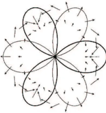
Leau and Fatou theorem. The dynamical picture appears as a flower where each petal is, alternatively, an attractive and repelling domain.

Figure 1: Leau-Fatou dynamics with three attractive petals and three re-pelling petals. The arrows go from z to f (z).

When f0_{(0) = e}2πiθ _{with θ ∈ R \ Q the germ is for almost every θ}

lin-earizable [52]. Cremer finds in [25] and [26] a family of maps that are not linearizable.

One of the goal of this work is to understand something more on dynamics of tangent to the identity maps in C2_.

`

Ecalle [31] and Hakim [36] proved that, if f is a germ of holomorphic diffeomorphism of Cn _{and df}

0 = Id, then generically there exist f −invariant

curves whose closure contains the origin and such that the dynamics is at-tractive (such curves are called parabolic curves for f in 0).

Successively Abate [2] proved the existence of such parabolic curves for

every germ tangent to the identity in C2_.

Abate technique retraces Seidenberg and Camacho-Sad strategy. In par-ticular Abate introduces an index Ind(f, S, p) for a diffeomorphism f at a point p of a curve S of fixed points and gets an index theorem, similar to the

(9)

Introduction 5

Camacho-Sad index one, that links the dynamics to the topological proper-ties of the curve. Abate, as Camacho and Sad, blows-up the map and reduces to the case of a map with a smooth curve of fixed points for which he can use the index theorem.

This formal analogy with the continuous dynamics theory was studied in more detail in [3], [11], [12]. In [3] and [11] Abate, Bracci and Tovena relate discrete and continuous dynamics (see Chapter 2) associating to a map a family of local vector fields, whose flows approximate, at the first order, the map. In [2], [11] and [12] the crucial concept of tangentiality of a map along a curve of fixed points is introduced (and generalized in [3]), i.e. something analogous to the ”continuous” concept of invariant curve for a vector field [28].

In [11] Bracci notes the possibility of simplifying Abate’s technique, as Cano did in case of foliation. So the presence of a (C1) or a (C2) point

guarantees the existence of a parabolic curve. A point that admits, in its resolution, a (C1) or (C2) point is called appropriate singularity.

At this point natural questions arise:

- by Camacho-Sad theorem we know that through every singularity of a holomorphic vector field a separatrix passes. So, when does another separatrix exist?

- given a diffeomorphism tangent to the identity with a singular curve of fixed points through which points does a parabolic curve pass?

We start with a holomorphic foliation (respectively a diffeomorphism tan-gent to the identity) with a separarix (respectively curve of fixed points) and we want to know if, and through which points, another separatrix (parabolic curve) passes.

(10)

Introduction 6

A first step in this direction is made by Bracci, that in [11] examines the case of generalized cusps, i.e., curves of type {yn _{= x}m_{}. The strategy}

consists in finding which conditions guarantee that a point is an appropriate singularity.

To make this we have to analyze the behavior of the index during the resolution of singularities of the foliation (map) but also of the separatrix (curve). This last analysis creates a lot of complications on the study of the evolution of the index, because we find points that can belong to one, two or even three irreducible branches of the total transform and in every of these cases the bheavior of the index changes.

An accurate study of the evolution of such index allows to state:

Theorem 0.1. Let M be a complex two dimensional manifold, F a

holo-morphic foliation on some open subset of M, S ⊂ M a possibly singular curve locally irreducible at a point p ∈ M, such that it is a separatrix for F at p. If Ind(F, S, p) 6∈ Q+ _{∪ {0} then there exists (at least) another}

separatrix for F at p.

The answer we find to the second question is specular to the previous one:

Theorem 0.2. Let M be a two dimensional complex manifold, f : M −→ M

a holomorphic map such that Fix(f ) = S with S a locally irreducible, possi-bly singular curve at a point p ∈ M. Assume that f is tangential on S and Ind(f, S, p) 6∈ Q+∪ {0}. Then there exists (at least) a parabolic curve for f at p.

These results generalize the results of Camacho-Sad and Abate. It is sufficient to perform a blow-up and remember that the self intersection of the exceptional divisor is −1 to find the conditions required by these theorems.

(11)

Introduction 7

Both results are of local flavour, in fact they allow to find exactly through which points a separatrix (parabolic curve) passes. We note that this criterion of localization is the same in the two contexts.

All these facts underline, another time, the strict relation between the two settings.

If this connection is so deep, as it seems, how can we read definitions and objects of one setting in the other one?

Differently from [2], [3] and [11], in [28] we associated to a germ f of diffeomorphism tangent to the identity, having a curve S of fixed points, a formal vector field X such that exp(X) = f .

Under this construction we have only to work with one vector field, in-stead of a family of vector fields as in [3] and [11], but we loose the con-vergence of the vector field. This construction is proposed even in a very recent preprint of Brochero Martinez, Cano and L´opez Hernanz [15]. These authors consider the case of a map with an isolated singularity. They, as always, make a blow-up and reduce to a map with a particular curve of fixed points, i.e. the exceptional divisor. According to the philosophical idea that the natural setting is a map with a generic curve of fixed points, we start with this general assumption. So we find their results as particular cases.

Naturally, this construction is useful only if we can get an index theorem for the vector field X which is exacltly the same of that of the map’s one. Such an index theorem might not exist for formal vector fields.

So, does the vector field X have some additional useful structure? To answer to this question let observe what happens when the vector field is the blow-up of a formal one and the invariant curve is the exceptional divisor. If

X := A(x, y) ∂

∂x + B(x, y) ∂ ∂y,

(12)

Introduction 8

where A, B ∈ C[[x, y]] then, when we formally blow-up X, in the chart

x = u; y = uv, the vector field becomes: A(u, uv) ∂

∂u +

µ

B(u, uv) − vA(u, uv) u

¶

∂ ∂v.

Now, it is easy to see that the coefficients of such vector field live in C[v][[u]] ⊕ C[v][[u]].

Namely, the coefficients are convergent (polynomial) in the coordinate

transver-sal to the exceptional divisor {u = 0}. This structure is preserved even in

the general case? The answer is positive and X is said transversely formal. Theorem 0.3. Let f be a germ of holomorphic diffeomorphism of C2 _with

F ix(f ) = S, where S is a non singular complex curve and suppose f is tangential to S. Then, the formal vector field X such that exp(X) = f is transversely formal along the separatrix S, namely

X ∈ C{x}[[y]] ⊕ C{x}[[y]].

The transversely formality is the right condition to get an index theorem of Camacho Sad type [28].

Theorem 0.4. Let X be a transversely formal vector field on a complex

manifold of dimension two tangent to a compact, connected non singular curve S ⊂ M. Then, for every p ∈ S there exists an index Ind(X, S, p) ∈ C such that:

X

p∈S

Ind(X, S, p) = S · S.

The existence of such an index allows to get the same dynamical result found for holomorphic vector fields, even for transversely formal ones.

(13)

Introduction 9 Theorem 0.5. Let A(x, y) ∂ ∂x + B(x, y) ∂ ∂y

be a transversely formal vector field with an invariant smooth curve S and let p ∈ S be such that Ind(X, S, p) 6∈ Q+ _{∪ {0}. Then there exists another}

formal separatrix through p.

If we want to study by mean of this construction the dynamics of maps with a curve of fixed points we need that the vector field X does not have a discrete set of singularities on the separatrix S. To reduce to this case we have to algebraically normalize it. Such an operation will be made very often and we refer to the new vector field as the normalization of X.

In this way, the condition of tangentiality assumes an easy geometric interpretation: f is tangent to S if and obly if S is invariant for the normal-ization of X along S.

This construction shows that the study of the evolution of the index during the reduction is the same for maps and vector fields. So, even by this way, we recover Theorem 0.2.

All the techniques used to study the dynamics of maps until now, always, refer to foliation techniques.

So a natural question arise: can all the parabolic curves be found by a blow-up process? Abate and Tovena in [5] noticed that the parabolic curves found in this way have an additional structure, in fact they survive under blows-up. Such parabolic curves are called robust parabolic curves. Abate and Tovena find in [5] a family of self-maps of C3 _{tangent to the}

identity and with the origin as an isolated fixed point with parabolic curves but with no robust parabolic ones. So in dimension three the two concepts are not the same. Until now we do not know if such difference exists even in dimension two. However, when we try to find an upper bound for the

(14)

Introduction 10

number of parabolic curves, with our method, we have to restrict to robust parabolic curves.

In [29] we study the dynamics flows of vector fields tangent to the identity . Such a set, denoted by Φ≥2(C2, 0), is a dense subset of the space of germs

of maps tangent to the identity in C2_{. In this work we give a geometric}

interpretation of some concepts of discrete dynamics, such as tangentiality, and examine with more attention the relationship of some concepts, such as dicriticity, for vector fields and maps.

We find that the concept of dicriticity passes from the map to the asso-ciated vector field and viceversa.

Proposition 0.6. Let f ∈ Φ≥2(C2, 0) be a map tangent to the identity in

C 2 _{and let X be the vector field such that exp(X) = f. Then f is dicritical}

in 0 if and only if X is dicritical in 0.

So we have that a dicritical map has infinitely many robust parabolic curves if and only if the vector field has infinitely many separatrices.

For what concerns the non dicritical case the robust parabolic curves are exactly the parabolic curves living inside a separatrix of the associated vector field:

Proposition 0.7. Let f ∈ Φ≥2(C2, 0) be a holomorphic map and let X be vector field such that exp(X) = f . Let ϕ be a robust parabolic curve. Then ϕ is contained in a formal separatrix of X. Conversely in every formal separatrix of X there exists at least one robust parabolic curve for f .

If we can estimate the number of robust parabolic curves inside a separa-trix and the number of separatrices, we get an upper bound for the number of robust parabolic curves. According to the work of Corral and Fernandez-Sanchez in [24] an upper bound for the number of separatrices exists and we find the following estimation for the number of robust parabolic curves.

(15)

Introduction 11

Theorem 0.8. Let f = (f1, f2) ∈ Φ≥2(C2, 0) be a non-dicritical holomorphic map. Set η(f ) := max{ord(f1 − Id), ord(f2 − Id)} and µ(f ) the Milnor

number of f. Then the number of robust parabolic curves is at most

(16)

Chapter 1 Continuous dynamics

In this chapter we recall the basic facts about holomorphic foliations. We start with the definition of a non singular foliation and then generalize it to the singular case, that is the most interesting case for this study. We end up by studying singular foliations in C2_.

1.1 Holomorphic foliations

In this section we briefly recall the basic definitions of holomorphic foliations. For more details we refer to [16], [17] and [34].

Definition 1.1. Let M be a complex manifold of complex dimension m.

A holomorphic foliation F on M of complex codimension k is given by a holomorphic maximal atlas

{ϕj : Uj → ϕj(Uj)}j of M such that the transition maps are of the form:

ϕj ◦ ϕ−1i :ϕi(Ui∩ Uj) → ϕj(Ui∩ Uj)

(17)

1.1 Holomorphic foliations 13

with gi,j and hi,j holomorphic maps. The charts ϕj are called trivialization charts.

Remark 1.2. A holomorphic foliation F is a real codimension 2k foliation

of M which is given by a holomorphic atlas of M whose transition maps preserve the complex structure.

Let us consider a real foliation F of real codimension k on an n + k manifold M, let ϕj : Uj → ϕj(Uj) be a chart as in the definition. The

plaques of F in U are given by ϕ−1_(R2n_{× {y}). Let P and ˜}_{P be two plaques}

of the charts ϕ and ˜ϕ. Then either P ∩ ˜P = ∅ or P ∩ (U ∩ ˜U) = ˜P ∩ (U ∩ ˜U).

On M we can define the following equivalence relation: two points p, q ∈ M are equivalent if and only if there are some plaques P1, · · · , Pr such that p ∈ P1, q ∈ Pr and Pi∩ Pi+1 6= ∅∀i.

Definition 1.3. A leaf of F is a class [p] ⊂ M under the previous introduced

equivalence relation.

Definition 1.4. The leaves of a holomorphic foliation F are the leaves of

the underlying real foliation.

Remark 1.5. The leaves, endowed with the natural complex structure,

be-come complex immersed submanifolds of M.

We can now recall what a singular foliation is.

Definition 1.6. A holomorphic foliation with singularities on a complex

manifold M is a pair F = (F0_{, X) where X ( M is a proper analytic subset} of M with codim(X) ≥ 2 and F0 _{is a (non singular) holomorphic foliation} on M0 _{= M \ X.}

The leaves of F are the leaves of F0 _{on M}0_{. The set X is called the}

(18)

Definition 1.7. A singular holomorphic foliation is called saturated if it is

not possible to find an analytic subset X0 _{⊂ X such that F}0 _{extends as a non} singular holomorphic foliation to M \ X0_.

1.1.1 Holomorphic foliations on complex surfaces

In complex dimension two it is easy to relate holomorphic foliations to holo-morphic vector fields [41], [47]. Let ζ be a holoholo-morphic vector field in a neighborhood of the origin U and suppose that Sing(ζ) = {0}. Let observe that if

ζ = A(x, y) ∂

∂x + B(x, y) ∂ ∂y

with {A(x, y) = 0} ∩ {B(x, y) = 0} = {0} then ζ defines a complex ordinary differential equation by:

˙ξ = ζ(ξ),

i.e. ₍

˙x = A(x, y) ˙y = B(x, y).

The set of solutions defines a singular foliation in U.

Viceversa, let F be a holomorphic foliation in a neighborhood U of the origin in C2 _{with Sing(F) = {0}. Let be p ∈ U \ {0} and define the function:}

f : U \ {0} → C p 7→ f (p),

where f (p) is the inclination of the complex line tangent to the leaf of F for

p in p. Such a function is a meromorphic function f : U \ {0} → C. Now we

recall two basic fact of complex analysis (see [35]):

Theorem 1.8 (Hartogs’ Theorem). Let M be a complex manifold, X ⊂

(19)

a meromorphic q-form in M \ X. Then ω admits a unique meromorphic extension ˜ω to M.

Theorem 1.9 (Cartan’s Theorem). In a neighborhood of a ball in Cn _with n ≥ 2 any meromorphic function f is the quotient of two holomorphic func-tions A and B such that {A = 0} ∩ {B = 0} has no components of positive dimension.

From this two theorems we easily deduce that f = A

B and

dy dx =

A(x, y) B(x, y).

so, the leaves of F are the integral curves of

A(x, y) ∂

∂x + B(x, y) ∂ ∂y.

Proposition 1.10. Any holomorphic foliation F in a neighborhood of the

origin of C2 _{can be given by a holomorphic vector field ζ and the singularities}

of F are the singularities of the vector field.

Let ζ be a holomorphic vector field in U ⊂ C2 _{such that {ζ = 0} contains}

some one dimensional component S and suppose S is described by a holo-morphic function h : U → C, i.e., S = {h = 0}. We can always assume that

h is reduced in the following sense: if a local function F vanishes on {ζ = 0}

then F = hm_F0 _{where m ∈ N and {F}0 _{= 0} ∩ {ζ = 0} has dimension zero.}

So we can write the vector field in the following way

hm_A 1 ∂ ∂x + h n_B 1 ∂ ∂y and so ζ = hm0ζ1,

(20)

where m0 _{= min{m, n} and ζ}

1 is a holomorphic vector field in U such that

{ζ1 = 0} has dimension zero. Thus the foliation Fζ admits an extension Fζ1

which satisfies Codim(Sing(ζ1)) = 2.

In conclusion we can always assume in case of foliations in C2 _that:

(i) the foliation, locally, is given by a holomorphic vector field;

(ii) the foliation is saturated, namely, it has only isolated singularities. Proposition 1.11. Let F be a saturated holomorphic foliation on M2_{. Then}

it exists an open covering {Ui} of M such that F|Ui is given by a holomorphic

vector field ζi in Ui and the number of singularities of ζi is at most one. For any i, j such that Ui ∩ Uj 6= ∅ there exists a holomorphic non vanishing function hi,j : Ui∩ Uj → C such that ζi = hi,jζj.

Remark 1.12. By the previous proposition we find a family of functions hi,j satisfying a cocycle condition. Thus defining a holomorphic line bundle L∗ over M and a natural morphism L → T1,0_{M (here L is the dual of L}∗_). This line bundle, L, is called the tangent bundle to the foliation. In fact, an equivalent way to define a holomorphic foliation on a two dimensional complex manifold M is by means of a holomorphic line bundle L over M and a morphism ϕ : L → T1,0_{M [34].}

Let us observe that on the open set Uj the vector field vj, defining the

foliation, in the local coordinates (z, w), assumes the form:

vj = Aj(z, w) ∂

∂z + Bj(z, w) ∂

∂w, (1.1)

for some Aj, Bj ∈ O(Uj). Therefore, vj, where vj 6= 0, generates the kernel

of the holomorphic 1−form ωj defined by:

(21)

1.2 Singularities and normal forms 17

In conclusion a holomorphic foliation in C2 _{(or more generally on a}

com-plex two dimensional manifold) can be seen as an equivalence class of vector fields or as an equivalence class [{Uj}j∈J, {ωj}j∈J]∼ of holomorphic 1−forms

where {{Uj}j∈J, {ωj}j∈J} ∼ {{Ui0}i∈I, {ωi0}i∈I} if and only if for every i, j

such that Uj ∩ Ui0 6= ∅ it exists a function, f ∈ O∗(Uj ∩ Ui0), such that ωj = f ω0

i.

1.2 Singularities and normal forms

A normal form for a holomorphic vector field is a particulary easy to handle expression of the vector field which we can obtain after some manipulations. If we are interested in the analytic (formal) structure of the vector field then the equivalence relation is the analytic (formal) conjugation.

Definition 1.13. Two germs of holomorphic vector fields (C2_{, 0), X}

1, X2 are

holomorphically (formally) conjugated if there exists a germ of holomorphic (formal) diffeomorphism Φ of (C2_{, 0) such that:}

dΦ ◦ X1◦ Φ−1 = X2.

If instead we were interested in the geometric structure determined by the vector field, i.e., in the foliation determined by the vector field, we can consider the following equivalence relation:

Definition 1.14. Two germs of holomorphic vector fields in (C2_{, 0), X} 1, X2

are holomorphical (formally) equivalent if there exists a germ of holomor-phic (formal) diffeomorphism Φ of (C2_{, 0) such that:}

dΦ ◦ X1 = Ψ · X2◦ Φ,

(22)

Remark 1.15. Let λ1, λ2 be the eigenvalues of the linear part of the

vec-tor field X. Up to conjugation, we can assume that the linear part of the vector field is diagonal (or triangular). This linear part is equivalent (if the eigenvalues are not both zero) to:

µ 1 0 0 λ2 λ1 ¶ .

According to the type of eigenvalues of the vector field we can divide the singularities in the following way:

Definition 1.16. Let X be a holomorphic vector field in (C2_{, 0) which is}

singular at the origin. Let λ1, λ2 be the eigenvalues of the linear part of X.

The singularity is

- in the Poincar`e domain if: 1. λ1λ2 6= 0; and

2. λ1

λ2 ∈ C \ R

−_.

- in the Siegel domain if: 1. λ1λ2 6= 0;

2. λ1

λ2 ∈ R

−_.

- a saddle-node if an eigenvalue is zero and the other is not zero; - a nilpotent singularity if both eigenvalues are zero but the linear part

is not zero i.e. the linear part is equivalent to x2_∂x∂₁.

1.2.1 Poincar`

e domain

In this section we recall some results of Poincar´e. The proofs can be found, e.g., in [19].

(23)

Theorem 1.17. Let X be a holomorphic vector field in (C2_{, 0) singular at}

the origin. Suppose that the singularity lies in the Poincar`e domain. If λ1

λ2 6∈ N ∪

1

N (where N1 = {n1 | n ∈ N \ {0}}) the vector field is holomorphically conjugated to its linear part.

The case in which λ1

λ2 ∈ N ∪

1

N was studied by Poincar`e and Dulac:

Theorem 1.18. Let X be a holomorphic vector field in (C2_{, 0). If} λ1

λ2 = n ∈

N ∪ 1

N, then X is holomorphically equivalent to:

(nx1+ axn2) ∂ ∂x + x2 ∂ ∂x2 .

1.2.2 Siegel domain

In this section we assume the singularity is in the Siegel domain i.e. the quotient of the eigenvalues is negative real. For the proofs we refer to [19]. Theorem 1.19. Let X be a holomorphic vector field in (C2_{, 0) which is}

singular at the origin. Suppose the singularity is in the Siegel domain. Then it is holomorphically conjugated to:

(λ1x1+ x1x2a(x1, x2)) ∂ ∂x1 + (λ2x2+ x1x2b(x1, x2)) ∂ ∂x2 , where a, b ∈ C{x1, x2}.

From a formal point of view we have:

Theorem 1.20. Let X be a holomorphic vector field in (C2_{, 0) singular at}

the origin and suppose the singularity is in the Siegel domain, then: 1. if λ1

λ2 ∈ Q

− _{the vector field is formally conjugated to:}

(λ1x1+ X k≥1 ψ1,kxnk+11 xkm2 ) ∂ ∂x1 + (λ2x2+ X k≥1 ψ2,kxkn1 xkm+12 ) ∂ ∂x2 ; 2. if λ1 λ2 ∈ R

(24)

1.2.3 Saddle node

Saddle-node singularities were first studied by Briot, Bouquet and Dulac [19], [30].

Theorem 1.21. Let X be a holomorphic vector field in (C2_{, 0) with a saddle}

node type singularity at the origin. Then is holomorphically conjugated to:

(x1+ x2g(x1, x2)) ∂ ∂x1 + (x2h(x1, x2)) ∂ ∂x2 , with g, h ∈ C{x1, x2}.

from the formal point of view we can say something more on the structure of g and h.

Theorem 1.22. Let X be a holomorphic vector field in (C2_{, 0) with a saddle}

node singularity at the origin. Then is formally conjugated to: xp+1₁ ∂ ∂x1 + (x2(1 + ωxp1)) ∂ ∂x2 , with p ∈ N and ω ∈ C.

1.2.4 Nilpotent singularity

In case of nilpotent singularities the problem of normal forms is more compli-cated and not completely solved. Generally, we have the Takens pre-normal forms:

Theorem 1.23 ([56]). Let X be a holomorphic vector field in (C2_{, 0) with a}

nilpotent singularity at the origin. Then is formally equivalent to:

(2x2+ xp1U(x1)) ∂ ∂x1 − nxn−1 1 ∂ ∂x2 , (1.3)

(25)

We can suppose that, up to conjugation, every nilpotent singularity is of the form: (x2+ a(x1)) ∂ ∂x1 + b(x1) ∂ ∂x2

with a(x1) = arxr1+ · · · and b(x1) = bs−1xs−11 + · · · .

Theorem 1.24 ([54]). The pre-normal form of Takens is analytic (i.e. the

series that reduces the vector field in the pre-normal form is convergent) if s < ∞.

In order to specify the structure of the function U we have to make some distinctions.

The numbers r and s are not invariant for the vector field but their relations are invariant. Thus we can make a classification of nilpotent singu-larities according to these relations:

1. we have a generalized cusp if bs−1 6= 0 and s < 2r;

2. we have a generalized saddle-node if ar 6= 0 and 2r < s;

3. we have a generalized saddle if s = 2r, ar 6= 0 and bs−1 6= 0.

Generalized cusp singularities have been classified by Str´o˙zyna and ˙Zol¸adek in [54]. To express such a classification we set:

XH = 2x2 ∂ ∂x1 + sxs−1 1 ∂ ∂x2 ; EH = 2x1 ∂ ∂x1 + sx2 ∂ ∂x2 n0 = r s − 1 2.

Theorem 1.25 ([54]). Let X be a holomorphic vector field in (C2_{, 0) with a}

(26)

is formally equivalent to one of the following normal forms Js

r,φ. These forms are classified by a formal series φ(x) = P∗cjxj (the star means that the summation is taken over a particular subset of integers), by the class modulo s of the exponent r 6= 0 or by r = ∞. - Js ∞,0= XH; - Js r,φ = XH + xr−11 (1 + φ(x1))EH, where X ∗ ₌ X j6=0,−r(mod s) , if r < ∞ e n0 6∈ Z;

- the vector field (1.25) where:

φ = cn0sx

n0s

1 ,

if r < ∞ e n0 ∈ Z;

- the vector field (1.25) where:

X ∗ ₌ X j∈{n0s,j0} + X j>j0 j6=0,−r(mod s), j6=j0+n0s .

If two vector field with normal forms Js r,φ e Js

0

r0_,φ0 are formally equivalent

then r = r0_{, s}0 _{= s}0 _{and φ(x}

1) ≡ φ(αx1) for some constant α that satisfies

α2r−s_{= 1, when r 6= ∞.}

The study of generalized saddle node is in [53]. Let consider:

n0 = s r − 2 EH = x1 ∂ ∂x1 + ry ∂ ∂x2 .

(27)

1.3 Desingularization theorem 23

Theorem 1.26 ([53]). Every holomorphic vector field with a generalized

sad-dle node singularity at the origin is formally equivalent to one of the fol-lowing normal forms Js,φ

r . Such forms are classified by the exponents s =

2r + 1, 2r + 2, · · · , ∞ and by the formal series φ(x1) =

P_∗ djxj1 : - J∞,0 r = (x2− xr1)∂x∂1; - Js,φ r = (x2− xr1)∂∂1 + x s−r−1 1 (1 + φ(x1))EH where X ∗ ₌ X j6=0(mod r) , if s < ∞ and n0 6∈ Z; - Js,φ r with φ = dn0x n0r 1 , if s < ∞ and n0 ∈ Z; - Js,φ r with: _X ∗ ₌ X j∈{n0r,j0} + X j>j0, j6=0(mod r), j6=j0+n0r ,

if s < ∞ and n0 ∈ Z and there exists a non zero coefficient dj0 with

j0 6= 0mod r.

If two vector field with a generalized saddle node singularity and with normal forms Js,φ

r and Js

0_,φ0

r0 are formally equivalent then r = r0, s = s0 and φ0(x1) ≡

φ(αx1) for some constant α such that αs−2r = 1.

1.3 Desingularization theorem

1.3.1 Blow-up of a complex surface

The blow-up of a complex surface M at a point p ∈ M consists of substituting the point p by a complex projective line, called exceptional divisor. In this way we find a new manifold of complex dimension two where, in place of p,

(28)

we have a complex projective line that we can interpret as the set of tangent directions of M at p. Let M be a complex surface, p a point of M and let TpM be the tangent space of M in p. Let:

[·] : TpM \ {0} −→

TpM \ {0}

∼ ∼= CP(1) where CP(1) is a complex projective line.

Let define:

Mp = (M − p) ◦

∪ CP(1)

and introduce on it a structure of differentiable manifold as follows.

If U is a coordinate open set of M that does not contain p then the corresponding chart on M is even a chart on Mp. If, instead, U is a coordinate

neighborhood of p in M and χ : U ⊆ M −→ C2 _{is a chart on M such that}

χ(p) = (x(p), y(p)) = (0, 0) we define:

V1 = (U − χ−1({0} × C )) ∪ (CP1− [K1])

V2 = (U − χ−1({0} × C )) ∪ (CP1− [K2])

where K1 = ker(dx)p and K2 = ker(dy)p, that is K1 =< [ _∂y∂ |p] > and K2 =< [_∂x∂ |p] > . Notice that V1∪ V2 = U and V1∩ V2 6= ∅. Let define:

χ1 : V1 −→ C2 q 7−→ µ x(q),y(q) x(q) ¶ , if q ∈ U − χ−1_{({0} × C )} · α1 ∂ ∂x|p+ α2 ∂ ∂y|p ¸ 7−→ µ 0,α2 α1 ¶ , if · α1 ∂ ∂x|p+ α2 ∂ ∂y|p ¸ ∈ CP1\ [K1]. and: χ2 : V2 −→ C2 q 7−→ µ x(q) y(q), y(q) ¶ if q ∈ U − χ−1({0} × C ) · α1 ∂ ∂x|p+ α2 ∂ ∂y|p ¸ 7−→ µ α1 α2 , 0 ¶ if · α1 ∂ ∂x|p+ α2 ∂ ∂y|p ¸ ∈ CP1\ [K2].

(29)

Then {(Vi, χi)}i=1,2 is an atlas for Mp.

The projection: πp :Mp −→ M u 7−→ ½ u if u ∈ M \ {p} p if u ∈ CP1

is a holomorphic function and, in local coordinates, assumes the form:

πp(u, v) = (u, uv) in V1 ,

πp(u, v) = (uv, v) in V2.

1.3.2 Desingularization of a foliation

Let consider a germ of holomorphic foliation in C2 _{which is singular at the}

origin. We have seen that it can be expressed in the following form: (

˙x = A(x, y) ˙y = B(x, y)

where A(0, 0) = B(0, 0) = 0. If we denote by ν the algebraic multiplicity of this equation at 0 ∈ C2_{, i.e. the least order of its expression at 0 ∈ C}2_{, then}

we can write the previous equation in the form: (

˙x = Aν(x, y) + Aν+1(x, y) + · · ·

˙y = Bν(x, y) + Bν+1(x, y) + · · ·

where Ai and Bi are the homogenous part, of degree i, of the power series

expression of A and B.

In the chart of the blown-up manifold for which the projection assumes the form π(u, v) = (u, uv) the foliation becomes:

  

˙u = Aν(u, uv) + Aν+1(u, uv) + · · ·

˙v = ˙y − v ˙u

u =

Bν(u, uv) + Bν+1(u, uv) + . . . − v(Aν(u, uv) + . . .)

(30)

or, in a better form: (

˙u = uν_(A

ν(1, v) + uAν+1(1, v) + · · · )

˙v = uν−1(Pν+1(1, v) + u(· · · )),

where Pν+1(x, y) = xBν(x, y) − yAν(x, y). If we use the other chart we find

another vector field that is equivalent to this one on the intersection. So, we have a global foliation on the blown-up manifold. We have two cases: the dicritical one and the non dicritical one.

In case Pν+1(x, y) ≡ 0 the singularity is called dicritical and the foliation

becomes: ₍

˙u = uν_(A

ν(1, v) + uAν+1(1, v) + · · ·

˙v = uν(· · · ).

Dividing by the factor uν _{we obtain a saturated foliation that is equivalent to}

the previous one outside (u = 0). Let observe that in this case the exceptional divisor (u = 0) is not invariant for the foliation.

In case Pν+1(x, y) 6≡ 0 we have a non dicritical singularity and to get a

saturated foliation we can only divide by uν−1_{. In this way the curve (u = 0)}

is an invariant curve for the foliation.

Let observe that in both cases we find a discrete set of singularities and so we can repeat the construction for every singularity. In this way we can reduce the vector field to have only a particular class of singularities: dicritical ones and reduced ones.

Definition 1.27. Let M be a complex surface, F an holomophic foliation

on M and p ∈ M, an isolated singularity of F. The point p is a reduced singularity for F if one of the following conditions holds:

(∗1) λ1 6= 0, λ2 6= 0 and λ_λ1₂ 6∈ Q+∪ {0}

(31)

1.4 Separatrices of foliations 27

Theorem 1.28 (Seidenberg Theorem [16], [43], [51]). After a finite

num-ber of blows-up we can reduced the foliation to one that has only dicritical singularities and reduced singularities.

1.4 Separatrices of foliations

Let us consider the foliation: (

˙x = 3y2

˙y = 2x.

The foliation is singular at (0, 0), the curve {x2_{− y}3 _{= 0} \ {(0, 0)} is a leaf}

for the foliation and its closure {x2_{− y}3 _{= 0} is a singular curve, containing}

(0, 0). In order to analyze such a situation we start with a definition:

Definition 1.29. Let M be a complex surface, F a holomorphic foliation on

M and p a point of M. A local separatrix of F at p is a germ of irreducible complex curve C ⊂ M, such that p ∈ C and C \ {p} is a leaf of F |_{M \Sing}_(F). Namely, if vj represents the foliation F on the open set Uj that contains the point p, then:

spanC{vj(q)} = TqC.

Remark 1.30. Let C be a separatrix for F. If j : C −→ M is the immersion

of C in M and the foliation, F, is defined by {ω = 0} with ω a holomorphic

1−form on M, then j∗_{(ω |}

C\{p}) ≡ 0.

If the point p is not a singularity for the foliation F then the Cauchy-Kowaleskaya theorem assures the existence of exactly one non singular com-plex curve C such that p ∈ C and C is a leaf of F. This means that a separatrix C is such that Sing(C) ⊂ Sing(F).

If the point p is a dicritical singularity then infinite separatrices pass trough it.

(32)

1.5 Camacho-Sad index theorem 28

Lemma 1.31 ([16]). Let M a complex surface and F an holomorphic

folia-tion on it. Let p be a point of M. If p is a dicritical singularity for F then there exist infinitely many separatrices through p.

In case of reduced singularity the problem of existence of separatrices can be solved using the normal forms we have described in the previous section. if p is a reduced singularity of type (∗1) then there exist exactly two sepa-ratrices passing through p and they intersect each other transversally, if p is a singularity of type (∗2) then there exist two formal separatrices

passing through p, one is always convergent and it is called strong separatrix, and the other is generally only formal and it is called weak separatrix.

1.5 Camacho-Sad index theorem

In this section we recall the Camacho-Sad index theorem [18] in its general form [55], [39]. Let S be a singular curve on a complex surface M and let suppose that S is compact and irreducible. Let F be a holomorphic foliation on M with a discrete set of singularities on S. Let S0 _{:= S \ (Sing(S) ∪}

Sing(F)).

Lemma 1.32 (Baum-Bott vanishing lemma for the Camacho-Sad theorem [39]). There exists a connection ∇ for the normal bundle NS0 of S0 in M,

such that its curvature K ≡ 0 on S0_.

By the previous lemma we can prove the following index theorem in case

S is even singular [39] [55] (Camacho and Sad proved the result only in

case S is not singular). The proof is based on the localization around the singularities of the curvature K of the previous connection.

(33)

1.6 Camacho-Sad and Cano results 29

Theorem 1.33 (Suwa, Lehmann [39], [55]). Let S be a compact irreducible

curve in M. Let F be a holomorphic foliation in M with Sing(F) discrete and such that S is F−invariant. Then for every point p ∈ Sing(F) ∩ S there exists a complex number Ind(F, S, p) ∈ C that depends only on the behavior of F near S in p such that:

X

p∈Sing(F)∩S

Ind(F, S, p) = S · S.

Moreover, if S is defined by {f = 0} at p, and F is defined by ω = f dτ +hdf =

0 at p, then: Ind(F, S, p) = 1 2πi Z L dτ h

where L = S ∩ S3 _{and S}3 _{is a sphere centered in p with a small radius.}

As we can see in the following section it will be convenient to use this index together with blow-up techniques. So we describe the behavior of the index under blow-up.

Proposition 1.34. Let M be a two dimensional complex manifold, F a

holomorphic foliation, S an F -separatrix and p ∈ Sing(S). We denote by π : ˜M −→ M the blow-up of M at p, by ˜F the saturated foliation and by D := π−1_{(p) and ˆ}_{S := π}−1_{(S \ {p}), respectively, the exceptional divisor} and the strict transform of S. Then ˆS is an ˜F separatrix. Moreover if {˜p} := D ∩ ˆS then

Ind( ˜F, ˆS, ˜p) = Ind(F, S, p) − m2

where m ≥ 1 is the multiplicity of S in p.

1.6 Camacho-Sad and Cano results

The general problem of the existence of a separatrix for holomorphic foliations on complex surfaces was solved by Cesar Camacho and Paulo Sad in 1982:

(34)

Theorem 1.35 (Camacho-Sad theorem [18]). Let M be a complex surface

and F a holomorphic foliation on M. Then through every singularity p of F passes at least a separatrix.

We recall the steps of the proof of this results:

1. study of the existence of separatrices through reduced singularities, 2. Seidenberg reduction theorem,

3. Index Theorem, 4. combinatoric part.

By Seidenberg theorem we can assume, after a finite number of blows-up, that all singularities on the exceptional divisor are only of type (∗1) or (∗2). In fact, in case of presence of dicritical singularities Lemma 1.31 assures the existence of infinite separatrices and so the problem is solved. Now, the prob-lem is that it could happen that all singularities of type (∗1) are intersections of irreducible components of the exceptional divisor and all singularities of type (∗2) are smooth points of the exceptional divisor that have not conver-gent weak separatrix. To prove that this situation cannot happen Camacho and Sad exploited an index theorem that link the singularities of F on every irreducible component of the exceptional divisor with the geometry of its immersion in the ambient space. By this tool and a combinatoric argument they proved that it must exist a good (∗1) singularity, i.e., a (∗1) singularity on an irreducible component of the exceptional divisor which is not a cor-ner. Thus, through this singulariy, there passes a separatrix which is not contained in the exceptional divisor and this projects down into a separatrix for the original foliation.

(35)

We quote here a result of Cano that is extremely useful to generalize the Camacho-Sad result [20].

M and S a separatrix of F through p ∈ M.

• the point p ∈ S is of type (C1) if S is not singular at p and

Ind(F, S, p) 6∈ Q+∪ {0}.

• the point p ∈ S is of type (C2) if S has exactly two irreducible non

singular branches S0, S1 that intersect transversally at p and there exists

a number r > 0 such that:

Ind(F, S0, p) ∈ Q≤−1

r := {x ∈ Q | x ≤ −

1

r} Ind(F, S1, p) 6∈ Q≥−r := {x ∈ Q | x ≥ −r}.

This class of points is stable under blow-up in the sense described by the following lemma.

Lemma 1.37 ([20]). Let M be a complex surface, F an holomorphic foliation

and S a separatrix for F passing through p ∈ M. Let suppose that p ∈ S is a point of type (C1) or (C2). Let π : ˜M −→ M the blow-up of M at p,

˜

S := π−1_{(S) the total transform of S and ˜}_{F the saturated foliation associated} to F. Then there exists a point of type (C1) or (C2) on ˜S.

According to this lemma we get the following definition:

M and S a separatrix of F trough p ∈ M. The point p is an appropriate singularity for F if after a finite number of blow-ups there exists a point of type (C1) or (C2) on the total transform of S.

(36)

In case we can find a (C1) or a (C2) point, Cano proves that if we blow-up

only these points, after a finite number of blows-up, we eventually find a good (∗1) singularity and thus we get the existence of a separatrix.

Proposition 1.39 ([20]). Let M be a complex surface, F a holomorphic

foliation and S a separatrix of F through p ∈ M. Let suppose that p ∈ S is an appropriate singularity for F. Then there exists at least a separatrix through p.

(37)

Chapter 2 Discrete dynamics

In this chapter we concentrate our attention on the dynamics of maps tangent to the identity in C2_{. Firstly, we recall how things work in dimension one.}

2.1 Discrete dynamics in dimension one

We recall some basic facts about complex dynamics in dimension one. For more details see [21], [45]. A formal diffeomorphism is every formal series

ˆ

ϕ ∈ C[[x]] such that ˆϕ(0) = 0 and ˆϕ0_{(0) 6= 0.}

Proposition 2.1. Let be f = az + . . . ∈ Diff(C, 0), a ∈ C∗ _{= C \ {0}. Then} there exists a formal change of coordinates, ˆϕ, such that:

1. ˆϕ∗f (z) := ˆϕ−1◦ f ◦ ˆϕ(z) = az, if a is not periodic, i.e. an6= a for every n ∈ N;

2. ˆϕ∗f (z) = az if a is of order q ∈ N∗_{, a}q _{= 1, and f}◦q _{= Id,} 3. ˆϕ∗f (z) = a exp(Xkq,λ) with k ∈ N∗ and Xp,λ = z

p+1 1+ λ 2πizp ∂ ∂z if a is of order q ∈ N∗ _{but f}◦q _{6= Id.}

(38)

2.2 Dynamics in C2 ₃₄

Theorem 2.2 (Koenigs). With the notations of the Proposition 2.1, if |a| 6= 1

then the conjugation to the linear part is holomorphic.

From a dynamical point of view is interesting to know what happen to the iterates of the map. With this aim we introduce the following definition: Definition 2.3. Let be f : D ⊂ C → f (D) ⊂ D an holomorphic map such

that 0 ∈ D and f (0) = 0. The map is attractive on D if for every p ∈ D

lim

n→+∞f

(n)_{(p) = 0,}

where f(n)_{:= f ◦ · · · ◦ f If the map is a diffeomorphism and f}−1 _{is attractive} on f−1_{(D) then the map is called repelling on D.}

According to this definition, if | f0_{(0) |6= 1, then the map is attractive (if} | f0_{(0) |< 1) or repelling (if | f}0_{(0) |> 1). So, from a dynamical point of view,}

the more interesting maps are those with | f0_{(0) |= 1.}

In this class of holomorphic maps the most important, for the intent of this thesis, are the maps tangent to the identity i.e. such that f0_{(0) = 1. The}

dynamics of these maps is completely described by the Leau-Fatou flower Theorem [45].

Theorem 2.4 (Leau-Fatou flower theorem). Let f (z) = z + akzk_{+ . . ., with} k ≥ 2 and ak 6= 0, be a holomorphic function fixing the origin. Then there are k − 1 disjoint domains D1, · · · , Dk−1 with the origin in their boundary, invariant under g (i.e.g(Dj) ⊂ Dj) and over which g is attractive.

2.2 Dynamics in C

2

We are interested in the study of the dynamics of germs of maps f of (C2_{, 0)}

tangent to the identity, i.e., df0 = Id. To find a dynamical behavior similar

(39)

2.2 Dynamics in C2 ₃₅

Definition 2.5. Let M be a complex surface, f : M → M a holomorphic

function and p a point in M. A parabolic curve for f at p is an injective holomorphic map φ : ∆ → M, with ∆ := {ζ ∈ C | |ζ| < 1}, satisfying:

(1) φ is continuous on ¯∆ and p = φ(1); (2) f (φ(∆)) ⊂ φ(∆);

(3) for all q ∈ φ(∆) limn→∞fn(q) = p.

We want to analyze the existence and the number of this objects. To get this goal we convert the problem in terms of continuous dynamics.

In the following sections we recall how to construct this dictionary fol-lowing [2], mainly [11] and [3].

2.2.1 Singularities of maps

Let M be a complex surface and p a point in M. Let f : M → M be a holomorphic function such that f (p) = p and dfp = Id.

For every z, w ∈ Op let us consider the 1−form:

ωw,z,p _{:= (w ◦ f − w)dz − (z ◦ f − z)dw,}

and construct the family of germs of holomorphic foliations: Ωf,p:= {ωw,z,p = 0 | w, z ∈ Op, dwp∧ dzp 6= 0}.

For every ωw,z,p _{∈ Ω}

f,p we can construct the form ˆωw,z,p dividing the given

form ωw,z,p _{by the greatest common divisor of the coefficients.}

Remark 2.6. ˆωw,z,p _{= ω}w,z,p _{if and only if p is an isolated fixed point of f .}

In this way we have linked the study of discrete dynamics to the contin-uous one.

(40)

2.2 Dynamics in C2 ₃₆

Definition 2.7. Let M be a complex surface. Let p be a point in M and

f : M → M a holomorphic function such that f (p) = p and dfp = Id. The point p is a singular point for f if ˆωw,z,p_{[p] = 0 for every ω}w,z,p _{∈ Ω}

f,p.

Using this construction we can translate to discrete dynamics all the defi-nitions given for foliations. In particular we still have points of type (∗1) and (∗2). Let us observe that the definition of (∗1) and (∗2) points is independent of the coordinates. The following lemma assures that the definition is well posed:

Lemma 2.8 ([11]). Let ˜w, ˜z ∈ Opbe such that d ˜wp∧d˜zp 6= 0 and let z, w ∈ Op with dzp ∧ dwp 6= 0. Then there exists u ∈ O∗

p such that ωz, ˜p˜w,p = uωpz,w,p. In particular if both the eigenvalues of the linear part are non zero, the quo-tient λ1z,w,p

λ2z,w,p is independent by z, w and if it exist z0, w0 such that one of the

eigenvalues λz0,w0,p

j = 0 then it holds for every z, w.

We can now give the definition of reduced singularities for maps.

Definition 2.9 ([2],[11]). Let M be a complex surface, p a point of M and

f : M → M a holomorphic map such that f (p) = p and dfp = Id. The point

p is a reduced singularity for f if it is a reduced singularity for some and hence for all ωz,w,p_{, i.e., one of the following conditions holds:}

(∗1) λz,w,p₁ λz,w,p₂ 6= 0,λz,w,p1

λz,w,p2 6∈ Q

+_,

(∗2) λz,w,p₁ = 0, λz,w,p₂ 6= 0 or λz,w,p₂ = 0, λz,w,p₁ 6= 0.

2.2.2 Curves of fixed points

Now we have to convert in the language of the foliation the case of a map with curve of fixed points. Let M be a complex surface and S a (possibly singular) irreducible curve in M. Let f : M → M be a holomorphic function such

(41)

2.2 Dynamics in C2 ₃₇

that f |S= IdS and f 6= IdM. Let U be an open set of M and φ : U → C 2

a local chart on M. If l ∈ Op is a defining function of the curve S near the

point p then:

φ ◦ f ◦ φ−1 = Id + (l ◦ φ)TG (2.1)

for some germ G = (G1, G2) of holomorphic function at p with G |φ(S)6≡ (0, 0)

and T ≥ 1.

The exponent T in the decomposition (2.1) is called order of f on S in

p and we denote it with Tp(f, S).

Remark 2.10 ([12]). We observe that ∀q ∈ U ∩S we have Tq(f, S) = Tp(f, S) .

If p ∈ U ∩ (S \ Sing(S)) the defining function l of S in p is such that

dlp 6= 0. Let τ be a function on U such that dτp∧ dlp 6= 0 (we say that τ is

transverse to l in p). So we can construct: ˆ

ωl,τ,p _:= τ ◦ f − τ alT dl −

l ◦ f − l alT dτ,

with a ∈ O(U), a |S6≡ 0. We see that S is a leaf of ˆωl,τ,p if and only if l◦f −l

lT ≡ 0 modulo the ideal of functions identically vanishing on S at p.

Definition 2.11. Let M be a complex surface, S an irreducible complex

curve (possibly singular) in M. Let f : M → M be a holomorphic function such that f |S= IdS and f 6= IdM. If p is a point of S we say that f is tangential on S at p if for every function l that defines S near p:

l ◦ f − l

lT ≡ 0 mod I(S)p. (2.2)

where I(S)p is the ideal of functions identically vanishing on S at p.

Proposition 2.12 ([12]). If the curve S is globally irreducible then f is

non-tangential at p ∈ S if and only if f is non-non-tangential at q ∈ S for every q ∈ S.

(42)

2.2 Dynamics in C2 ₃₈

In terms of foliations we can read the tangentiality conditions in the following way:

Proposition 2.13 ([11]). The map f is tangential on S ∩ U if and only if S

is a leaf for the family of holomorphic foliations on U given by {ωl,τ_{} where:} ωl,τ := τ ◦ f − τ

lT dl −

l ◦ f − l lT dτ, for any defining function l of S and transverse to S τ .

Assumes f is tangential on S. If p ∈ Sing(S) then dlp = 0 for any

defining function of S at p. Therefore in this case ωl,τ_{[p] = 0 for any defining}

function l of S and any transverse τ . So p is a singularity for all the family of foliations ωl,τ _{= 0. Also in this case we say that p ∈ S is a singularity of} f .

Now we can define even dicritical singularities for maps. To do this we have to define how to transfer the map f on the blown-up surface ˜M. In [1]

Abate proves that there exists a unique ˜f : ˜M → ˜M such that π ◦ ˜f = f ◦ π

and whose action on the exceptional divisor is induced by the action of dfp

on P(TpM).

Definition 2.14. Let M be a complex surface, p a point of M and f :

M → M a holomorphic function such that f (p) = p and dfp = Id. Let π : ˜M → M be the projection of the blow-up of M in p and let D := π−1_(p) be the exceptional divisor. The point p is dicritical for f if ˜f : ˜M → ˜M is non tangential on D.

After these definitions we can expect that even a sort of reduction of singularities holds for maps. Indeed:

Theorem 2.15 ([11] [2]). Let M be a complex surface, S a (possibly singular)

(43)

2.2 Dynamics in C2 ₃₉

map such that f (p) = p and dfp = Id. Then there exists a complex surface

˜

M, a holomorphic proper function π : ˜M → M and a holomorphic function

˜

f : ˜M → ˜M such that:

(1) D := π−1_{(p) = ∩}n

i=1Di where Diare complex projective line that intersect each other transversally;

(2) π : ˜M \ D → M \ {p} is a biolomorphism;

(3) π ◦ ˜f = f ◦ π;

(4) ˜f |D= Id |D;

(5) ˜f has only reduced singularities or dicritical singularities on D.

2.2.3 Index Theorem

In the previous section we introduced a link between separatrices and curves of fixed points. We know that in the study of separatrices is extremely useful to have an index theorem. So one of the first step in the study of discrete dynamics is to find an index theorem [2], [3], [11].

Using the foliations {ωl,τ _{= 0} defined before and observing that all the} {ωl,τ _{= 0} are equal to the first tangential order in S [2], [11], we find that:}

Theorem 2.16 ([2] [11] [12]). Let M be a complex surface, S a globally

irreducible compact complex curve and f : M → M a holomorphic function such that f |S= IdS and f is tangential on S. Then for every p ∈ S there exists a number Ind(f, S, p) ∈ C, that depends only on f near S in p, such that:

X

p∈S

(44)

2.2 Dynamics in C2 ₄₀

If l defines S in p and τ is transversal to l the index assumes the form: Ind(f, S, p) = 1 2πi Z ∂L ½ l ◦ f − l l(τ ◦ f − τ ) ¾ dτ,

where L = S3_{∩ S with S}3 _{a sphere centered in p with enough small radius.}

As for foliation we want to use the index theorem together with blow-up techniques. So it is useful to know the behavior of the index under blow-up. Proposition 2.17 ([11], [12]). Let M be a complex surface, f : M → M

a holomorphic function and S a curve in M such that f |S= IdS and f is tangential on S. Let p ∈ S be a point such that S is irreducible at p and let π : ˜M → M be the blow-up of M in p and ˜f : ˜M → ˜M the induced map by f . If D := π−1_{(p) is the exceptional divisor and ˆ}_{S := π}−1_{(S \ {p}) the strict} transform of S then:

(1) the map ˜f is tangential on ˜S,

(2) if {˜p} = D ∩ ˜S then Ind( ˜f , ˆS, ˜p) = Ind(f, S, p) − m2 _{where m ≥ 1 is the}

multiplicity of S in p.

2.2.4 Parabolic curves

The constructions made until now suggest to retrace the proof of Camacho-Sad [18] to get the existence of parabolic curves. To make this we need the last ingredient i.e., the solution of the problem for some particular cases.

If the point p is not a singularity the problem was solved by Abate [2]: Proposition 2.18. Let M a complex surface, S a curve in M and f : M →

M a holomorphic map such that Fix(f ) = S near p. Let suppose that f is tangential on S. If p is not a singularity for f on S then p is not an attractive point for f and then there do not exist parabolic curves for p.

(45)

2.2 Dynamics in C2 ₄₁

If instead p is a singularity of f of type (∗1) a first result is achieved by Hakim [36] (see also Abate [2] where a slightly simpler proof is given): Proposition 2.19. Let M be a complex surface, S ⊂ M a complex curve.

Let f : M → M be a holomorphic map such that f |S= IdS. Let p be a non singular point of S and suppose f is tangential on S at p. If Fix(f ) = S near p and p is a reduced singularity of type (∗1) for f then there exists at least one parabolic curve for f at p.

The last special case is the dicritical one:

Proposition 2.20 ([2], [11]). Let M be a complex surface, p ∈ M. Let

f : M → M be holomorphic and such that f (p) = p, dfp = Id. Then p is dicritical for f if and only if there exist infinitely many parabolic curves for f at p.

Now we have all the ingredients for the general case. We can desingular-ized the map f around an isolated singularity. At the end, if we do not find dicritical singularities, we find a good (∗1) singularity and then there exists a parabolic curve that projects into a parabolic curve for f . With this strategy in mind we can follow Cano’s construction as proposed by Bracci in [11]. Definition 2.21. Let M a complex surface, S ⊂ M a complex curve. Let

f : M → M be a holomorphic map such that Fix(f ) = S.

• the point p ∈ S is of type (C1) if S is non singular in p, the map f is

tangential on S in p and

Ind(f, S, p) 6∈ Q+∪ {0}.

• the point p ∈ S is of type (C2) if S has two non singular branches S0, S1

On the relations between discrete and continuous dynamics in C2

University of Pisa

Faculty of Mathematical, Physical and Natural Sciences

Academic year 2005 - 2006

PHD Thesis

On the relations between

discrete and continuous

dynamics in C

2

Francesco Degli Innocenti

Advisor:

Prof. Filippo Bracci

President of doctorate:

Contents

Introduction

Chapter 1

Continuous dynamics

1.1

Holomorphic foliations

1.1.1

Holomorphic foliations on complex surfaces

1.2

Singularities and normal forms

1.2.1

Poincar`

e domain

1.2.2

Siegel domain

1.2.3

Saddle node

1.2.4

Nilpotent singularity

1.3

Desingularization theorem

1.3.1

Blow-up of a complex surface

1.3.2

Desingularization of a foliation

1.4

Separatrices of foliations

1.5

Camacho-Sad index theorem

1.6

Camacho-Sad and Cano results

Chapter 2

Discrete dynamics

2.1

Discrete dynamics in dimension one

2.2

Dynamics in C

2.2.1

Singularities of maps

2.2.2

Curves of fixed points

2.2.3

Index Theorem

2.2.4

Parabolic curves