Astrocook: a thousand recipes to cook a spectrum

(1)

2018

Publication Year

2021-02-10T10:31:09Z

Acceptance in OA@INAF

Astrocook: a thousand recipes to cook a spectrum

Title

CUPANI, Guido; CALDERONE, GIORGIO; CRISTIANI, Stefano; DI

MARCANTONIO, Paolo; D'ODORICO, Valentina; et al.

Authors

10.1117/12.2312093

DOI

http://hdl.handle.net/20.500.12386/30269

Handle

PROCEEDINGS OF SPIE

Series

10707

Number

(2)

PROCEEDINGS OF SPIE

SPIEDigitalLibrary.org/conference-proceedings-of-spie

Astrocook: a thousand recipes to

cook a spectrum

Guido Cupani, Giorgio Calderone, Stefano Cristiani,

Paolo Di Marcantonio, Valentina D'Odorico, et al.

Guido Cupani, Giorgio Calderone, Stefano Cristiani, Paolo Di Marcantonio,

Valentina D'Odorico, Giuliano Taffoni, "Astrocook: a thousand recipes to

cook a spectrum," Proc. SPIE 10707, Software and Cyberinfrastructure for

Astronomy V, 1070723 (6 July 2018); doi: 10.1117/12.2312093

(3)

Astrocook: a thousand recipes to cook a spectrum

Guido Cupani

a

_{, Giorgio Calderone}

a

_{, Stefano Cristiani}

a

_{, Paolo Di Marcantonio}

a

_{, Valentina}

D’Odorico

a

_{, and Giuliano Ta↵oni}

a

_{INAF–Osservatorio Astronomico di Trieste, Via G. B. Tiepolo 11, I-34143 Trieste, Italy}

ABSTRACT

Astrocook is a new Python package to analyze the spectra of quasi-stellar objects (QSOs) from the near-UV band to the near-infrared band. The project stems from the lessons learned in developing the data analysis software for the VLT ESPRESSO spectrograph. The idea is to leverage numerical libraries like SciPy, NumPy, and Lmfit and astronomical libraries like Astropy to produce a collection of high-level recipes capable of interpreting the features observed in QSO spectra (such as the emission continuum and the absorption systems) in an automated and validated way. The package provides great flexibility in designing the operational workflow, as well as a set of interactive tools to apply the recipes in a seamless way. The aim is to achieve the combination of accuracy, stability, and repeatability of the procedure that is required by several compelling science cases in the era of ”precision cosmology” (e.g. the measurement of a possible variability in the value of fundamental constants, and the direct measurement of the accelerated expansion of the Universe).

Keywords: Astrocook, QSO spectroscopy, Data Analysis, Python package, Automatic workflow

1. INTRODUCTION

Astronomical spectroscopy is steadily evolving into a precision science. Present-day instrument are addressed to meet outstanding requirements in term of stability and repeatability of the observations, combining high resolution (R > 50, 000) with extreme wavelength calibration accuracy ( = 2⇥ 10 6_{nm at} _{= 550 nm).} The technological challenge is motivated by the exciting opportunities expected from the full exploitation of the visible spectra of quasi-stellar objects (QSOs) at a redshift between 2 and 6, both in the field of observational cosmology and fundamental physics.

The year 2018 saw the commissioning of the Echelle SPectrograph for Rocky Exoplanets and Stable Spectral Observation or ESPRESSO1 _{at the ESO Very Large Telescope (VLT). With its extreme thermo-mechanical}

stability (down to the mK and µPa scale), ESPRESSO is meant to pave the way to the future generation of spectrograph, like the Hi-Res spectrograph2,3_{for the ESO Extremely Large Telescope (ELT), currently}

under-going Phase A study. The science cases that such instruments are meant to address includes two very ambitious, possibly paradigm-changing experiments, namely:

• the measurement of a possible time variation in the value of dimensionless constants like the fine structure constant (↵) and of the proton-to-electron mass ratio (µ);4

• the Sandage test,5_{i.e. a purely-geometric measurement of the accelerated expansion of the Universe from}

a drift in the redshift of distant objects.

Both experiments involve an accurate interpretation of the features observed in the spectra of background sources, like QSOs. In the case of the Sandage test, the process of data acquisition and treatment must be prolonged under controlled conditions throughout a time span of 20 years, with some 4000 h of observation over a suitable catalog of targets. This poses unprecedented constraints not only on the design of the instrument hardware, but also on the software tools to handle its data output.

Send correspondence to Guido Cupani

Guido Cupani: E-mail: guido.cupani@inaf.it, Telephone: +39 (0)40 3199 235

(4)

It is no wonder that ESPRESSO was initially conceived as a “science machine” with a data treatment package explicitly included among its deliverable subsystems. This package includes both a Data Reduction Software or DRS and a Data Analysis Software or DAS.6–9 _{The combination of DRS and DAS is a first occurrence for an}

ESO instrument and is meant to provide the users not only with calibrated data products, but also with scientific measurements within minutes from the execution of the observations. The same approach will be followed for Hi-Res. A limited set of science objectives, combined with the unparalleled demands they entail, naturally favors the development of a dedicated analysis tool. On the other hand, there no reason not to extend the new algorithms designed to extract scientific information from a particular instrument to a more general framework. This is where the Astrocook project comes into play.

Astrocook10 _{is a Python}11 _{package to analyze QSO spectra. The name was originated by the tagline “a}

thousand recipes to cook a spectrum”, which is meant to emphasize the versatility of the tool. Astrocook relies on SciPy, NumPy,12_{and Lmfit}13_{for numerical computation and on Astropy}14_{for astronomy-related data}

handling. A working copy of the package can be downloaded for beta-testing from its GitHub webpage (https: //github.com/DAS-OATs/astrocook). Astrocook stems from the lessons learned in developing the ESPRESSO DAS, and is meant to extend its functionalities to virtually any available QSO spectrum. It provides both a collection of methods meant to be scripted by the users and a graphical user interface with more sophisticated analysis “recipes”. The aim of the project is twofold:

• presently, to allow for a combined analysis of data from ESPRESSO and from other instruments;

• in perspective, to validate and extend the algorithm developed for the DAS (also on simulated data), thus laying the foundation for the ELT Hi-Res data analysis tool.

This article provides an introduction to the features of Astrocook as of May 2018. It first discusses the main algorithms for QSO spectral analysis implemented in the code (Sect.2) and then describes the core structure of the package (Sect.3) and its graphical user interface (Sect.4). An outline of the future development of Astrocook is given in Sect.5.

2. ALGORITHMS FOR QSO SPECTRAL ANALYSIS

The analysis of QSO spectra is an inherently complex problem. Most of the information needed by the science cases outlined in Sect.1is obtained by modeling the absorption features which are produced by the inter-galactic medium (IGM) lying along the line of sight towards the QSO. These features are produced by di↵erent ionic transitions and may be associated with each other into systems, tracing the multi-phase IGM at di↵erent redshifts. The di↵erent phases may have di↵erent spatial structure, density, and dynamics, as can be inferred from a Voigt-profile fitting of the absorption lines they produce (see Sect.3.3). Absorption systems may be blended with each other across the sight line, or give rise to notable pattern such as the “forest” of lines produced when neutral hydrogen atoms are excited from their ground state by the absorption of UV photons (Lyman forest).

A correct interpretation of the absorption features requires a prior modeling of the emission continuum of the QSO, which in turn can be ideally reconstructed only by removing all the absorption features. To break the circle, one needs to model the absorption systems with respect to a guess continuum and to adjust the continuum itself using the best-fitting parameters through several iterations, until convergence is achieved. This approach is implemented in the ESPRESSO DAS by splitting the procedure into basic operations and allowing for a repeated execution of the following one-way pipeline:8

Line detection Continuum estimation System identification System fitting

In addition, the code embeds one further iteration scheme for the continuum estimation in the Lyman forest, using the estimated column density distribution of the absorption lines to progressively adjust the e↵ective optical depth of the neutral hydrogen, used to guess the unabsorbed continuum level. The underlying principle was to construct an automatic tool that mimicked as much as possible what human observers would perform “by

(5)

hand”. Other manual operations—e.g. using a detected metal-line doublet as a starting point to identify other lines, or adding components to a line-profile model to compensate for residuals between model and data—were reproduced in the code to be sequentially performed along a whole spectrum or across a catalogue of spectra. While successful when applied within its scope, the DAS approach shows some notable drawbacks:

• the granularity of the operations cannot be adjusted at will, and is generally too coarse to accommodate additional procedures into the code;

• all algorithms (for line detection, continuum estimation, system identification) are provided as closed box and allow for limited customization;

• the adopted graphical user interface (ESO Reflex15_{) is not meant to operate outside the one-way pipeline}

model.

More specifically, the DAS code is written to be embedded within the VLT data flow system, taking advantage of the ESO Common Pipeline Library (CPL);16 _{this limits its portability outside the ESO environment. The}

Astrocook concept is meant to address all these drawbacks at once.

3. THE ASTROCOOK CORE

The Astrocook core classes are designed around a very general definition of analysis: extracting information from a spectrum. At present, the information to be extracted is identified with the output of the ESPRESSO DAS (list of lines, continuum models, fitted absorption systems), but it is meant to be easily extended to di↵erent purposes.

The main class is Spec1D, which defines the structure of a spectrum; other relevant classes are Line and System, defining lists of lines and lists of absorption systems, respectively, and Cont, defining the QSO continuum model. A conceptual map of the relationship between classes can be outlined as follows:

Spec1D Line

System

Cont

The idea is that a list of line is necessarily derived from a spectrum, and that it can be used to define a list of absorption systems and to determine a model for the continuum; in turn, the defined systems can help refine both the list of detected lines and the continuum model. Objects of the di↵erent classes are constructed by keeping track of their provenance; e.g. a line list line always possesses an attribute line. spec containing the spectrum from which it has been extracted, and similarly a system list syst always possesses the associate attributes syst. spec, syst. line, and syst. cont. Every time an analysis procedure refines the interpretation of a given object, the information is propagated to the associated objects; e.g. when the system syst is fitted, any change in the continuum required by the fit is passed on to syst. cont.

3.1 The spectrum class

A Spec1D spectrum is an Astropy Table with obligatory X and Y columns, wavelength and flux density respectively. The columns are deliberately nondescript to serve equally well both wavelength spectra and frequency spectra; Xcan be any quantity dimensionally consistent with a wavelength or a frequency, and similarly Y can be a flux density expressed in any reasonable unit. The other columns of the table store the uncertainties DX and DY and the spectral resolution RESOL = / .

A Spec1D object is typically constructed from a FITS table, provided it possesses two columns that can be interpreted as X and Y. A spectrum can be also constructed from user-provided arrays X and Y. The class includes methods to perform the following operations:

(6)

• converting the X column into di↵erent units of wavelength and frequency; • converting wavelengths from air to vacuum;

• converting wavelengths from the Earth’s reference frame to the heliocentric or barycentric frame; • extracting a sub-spectrum with an X range of choice;

• convolving the flux density with a 1-d filter;

• finding the local extrema (maxima and minima) of the flux density;

• de-reddening the spectrum using the Astropy Specutils extinction package.17

3.2 The line list class and the continuum class

A Line list is an Astropy Table containing information about a set of emission or absorption line, one per row. Obligatory columns are X and Y—same as for spectra—with their uncertanties DX and DY, and a range XMIN-XMAX defining the region of spectrum a↵ected by the line.

A list of candidate absorption lines is extracted from the spectrum by looking for the most prominent local maxima (for emission) and minima (for absorption). Maxima and minima are determined after convolving the spectrum with a smoothing kernel (see Sect.3.1, and their prominence is computed as a multiple of the local flux density variance (typically at 5 ); as remarked in Sect.2, the definition of lines is heavily dependent on the scale considered, and di↵erent line lists are produced with a di↵erent choice of the smoothing parameters. For each candidate line, the neighboring extrema are used to define the range XMIN-XMAX (the closest minima for an emission line; the closest maxima for an absorption line). A more sophisticated definition of XMIN-XMAX based on the line equivalent width is under implementation. A Line object can be also constructed from a FITS table or from user-provided arrays.

The main operations available through the methods of this class are:

• finding the spectral lines in a spectrum with the algorithm described above;

• converting wavelength into redshifts and vice-versa, assuming the lines are produced by given ionic transi-tions;

• removing absorption lines from a spectrum, either masking the a↵ected regions or using a fitting profile to recover the unabsorbed emission level.

The latter method of the Line class can be used to construct a model of the continuum emission; this is actually done by one of the methods of the Cont class. A Cont spectrum is indeed a model of the QSO emission continuum; its structure is the same as a Spec1D spectrum, but containing only columns X, Y, and DY. A guess continuum is estimated by smoothing the distribution of the flux density local maxima after line removal and a kappa-sigma clipping of the outliers. Such continuum is meant to be refined during line fitting (see Sect.3.3); a more sophisticated technique developed for the Lyman forest is currently being ported from the ESPRESSO DAS (see Sect.2). Other

3.3 The system list class

A System list is an Astropy Table containing information about systems of associated absorption lines. These systems are produced by the large-scale structure of the IGM and are detected by looking for coincidences in redshift between lines produced by di↵erent transitions (of both hydrogen and metal ions). Astrocook defines absorption systems in a narrow sense, as sets of lines with the same redshifts, e.g. multiplets like the Civ 1548-1550 and the Mgii 2796-2803 doublets, or the Lyman series. Non-exact associations, like e.g. between a Lyman-↵ line and a Civ 1548-1550 doublet are listed as separate entries in the System Table. The individual components of a complex systems are also treated as separate systems, but they are considered together when they are fitted with a composite line profile.

(7)

The optical depth of absorption ⌧ systems is modeled as a function of the redshift z, the column density N , and the Doppler broadening b (both thermal and turbulent) of the absorbing medium. The profile of each component is obtained as I (z, N, b) = I ,0e ⌧ = I ,0  N p ⇡e2 mec f rf b V , (1)

where I ,0is the flux density of the emission continuum, f and rf are the oscillator strength and the rest-frame wavelength of the component, and V is the Voigt function:

V = a ⇡ Z +1 1 exp( y2₎ a2_{+ (u} _y)2dy, a := rf 4⇡b, u := c b  rf(1 + z) 1 , (2)

with the transition damping constant of the component. In a composite model, the optical depth terms are computed individually and the overall profile is computed as I (z, N, b) = I ,0e

P

i⌧ ;i_.

The Astrocook approach to the modeling and fitting of the absorption systems is similar to what implemented by other software packages (like Midas FITLYMAN,18_VPFIT,19_{and the more recent VoigtFit}20_{), with the added}

benefit of a graphical user interface (see Sect.4). The columns of the System table contain the information to construct a model of the system, namely the SERIES of components (e.g. [CIV 1548, CIV 1550]), the Voigt parameters Z, N, B, BTUR with their uncertainties DZ, DN, DB, DBTUR, a flag VARY to indicate which parameters are free to vary and which are fixed, and a set of expressions EXPR to link the parameters with each other (all components of a multiplets are fitted with the same values of the Voigt parameters). The System object is always associated with a Line object, listing the wavelengths X and the flux densities Y of the lines of each system. Such Lineobject is either the original list of lines detected on the spectrum (if the System object was created from a list of lines) or a synthetic line list created extracted from the system list itself (if the System object was constructed from a FITS table or from user-provided data).

The class provides methods to perform, among others, the following operations:

• finding systems in a list of lines, by finding coincidences between redshift values that can be computed from the lines wavelength, considering a given transition;

• grouping systems and individual lines that must be considered together when fitting a given system (these are all lines whose XMIN-XMAX range intersects the range of the lines in the system);

• extracting the spectral regions to be considered when fitting a given system; • modeling a system with a composite Voigt profile;

• computing the best-fitting parameter for a given model, using the Lmfit Levenberg-Marquardt minimizer. The methods, combined with the LMFIT interface, allow for a great degree of control of the parameters, including the normalization of the emission continuum I ,0, in the fitting of individual systems. The insertion or deletion of systems, needed to improve the fit chi-squared-wise, is done either manually, through a graphical user interface (see sect.4), or automatically by dedicated methods.

4. THE GRAPHICAL USER INTERFACE

One of the drawbacks of the past (e.g. ESO MIDAS, IRAF, etc.) and present-day data analysis tool is the steep learning curve required to produce powerful scripts within the chosen environment. With Astrocook, the widespread knowledge of the Python language mitigates this weakness; nevertheless, the subtlety of some analysis operations, like the design of a suitable composite model to be fitted to a complex absorption system, are better addressed by graphical means.

Astrocook is provided by a full-fledged graphical user interface (GUI) to perform the operations that can be performed through scripting. Though in its infancy, the GUI is meant to provide the primary access to the Astrocook package, especially as it grows to include a wider range of procedures. In addition, the GUI makes

(8)

pet

o1

Lines

Extract Spectral Region... Find Lines...

Find Continuum by Removing Li

hi acti ige]nm] system

1641.95,781.49]

Systems

76 19 Find Systems...

Fit Selected System...

X XMIN XMAX Y DY SERI Z R B BTIIR U2 UM DB DBTUR 1 643.952 642.630 644.236 10.123 0.230 1 MgII 1.45704 1.000e+14 10.000 0.000 nan nan nan nan 2 648.100

650.554

647.720 648.409 10.258 0.235 2 MgII 1.46074 1.000e+14 10.000 0.000 nan nan nan nan

3 650.077 650.865 5.228 0.148 3 MgII 1.46697 1.000e+14 10.000 0.000 nan nan nan nan

4 651.629 651.223 652.036 10.588 0.223 4 MgII 1.48948 1.000e+14 10.000 0.000 nan nan nan nan

5 653.977 653.401 654.265 10.278 0.199 5 MgII 1.66562 2.559e+16 33.184 0.000 0.00001 7.191e+16 7.099 0.000

l

9 666.109 665.841 666.280 9.321 0.177 9 MgII 1.76066 1.000e+14 10.000 0.000 nan nan nan nan 10 666.721 666.280 667.039 4.352 0.138 10 MgII 1.76517 1.000e+14 10.000 0.000 nan nan nan nan

11 669.491 669.024 669.982 6.754 0.163 11 CIV 3.20197 1.000e+14 10.000 0.000 nan nan nan nan 12 670.130 669.982 670.277 9.403 0.180 12 CIV 3.22950 5.000e+1910.000 0.000 nan nan nan nan

14 12 6 - 8 LL 6 4 2 700 710 720 Wavelength Mm 730 740 750

*

1+IQ 31®I

Plot

I

Clear

Figure 1. The Astrocook GUI main canvas, with a portion of a QSO spectrum displayed together with the associated line list and absorption system list. The recipe menu is also shown.

available a set of more complex operations—“recipes”—obtained by combining methods of the Astrocook core classes and accessible also as methods of the App class. The GUI recipes are meant to provide access to common functionalities in a seamless way.

In this section, the Astrocook GUI is described in reference to some specific use cases.

4.1 Basic operations

An example of the Astrocook in use is shown in Fig.1. The main canvas is split into four regions:

• the Spectra panel at the top, listing all the spectra loaded for analysis together with some basic information (target name, emission redshift, number of detected lines and absorption systems when applicable); • the Lines panel at the center left, listing all the detected lines for the currently selected spectrum; • the Systems panel at the center right, listing all the identified absorption systems for the currently selected

spectrum;

• the Plot panel at the bottom, displaying the spectrum at the current state of analysis (e.g. with crosses highlighting the position of the lines and with the estimated continuum superimposed, when applicable). A new analysis session is started by loading a spectrum from a FITS file through the File menu. Several spectra can be loaded at once and alternatively selected from the Spectra panel. The Plot panel is updated at runtime

(9)

whenever a new spectrum is selected. As the analysis progresses, the Lines and Systems are also updated in sync. Both table can be edited by the users at their own discretion. When a line or a system is selected on the table, its position is interactively highlighted on the plot. The user can clear and refresh the plot and interact with it using the Matplotlib21_{toolbar at the bottom left corner.}

Analysis sessions can be saved at any time through the File menu as a tar gzip archive (with extension .acs). The archive includes the Spec1D, Line, Cont, and Syst objects created during the session, providing a snapshot of the ongoing analysis to be retrieved at a later time. Di↵erent snapshots can be loaded concurrently in the Spectra panel and carried on independently.

The Recipes menu currently allows to launch the following operations:

• extracting a spectral region from a spectrum, either based on the QSO emission redshift (e.g. Lyman forest, Cii forest, etc.) or on a user-provided wavelength range;

• finding lines in a spectrum (see Sect.3.1and3.2);

• determining a guess continuum by removing the absorption lines (see Sect.3.2); • identifying absorption systems in a list of lines (see Sect.3.3);

• fit the selected systems with composite Voigt profiles (see Sect.3.3).

Each recipe is managed by a dedicated dialog window to tune the parameters of the algorithm. After the recipes are run, the information in the main canvas is updated: in particular,

• spectral regions extracted from a spectrum are displayed as separate entries in the Spectra panel and denoted by their active range in the dedicated columns;

• the line table is rewritten from scratch every time the recipe Find Lines is executed (a recovery option is available to undo this potentially disruptive operation);

• the system table is incrementally updated every time the recipe Find Systems is executed, to allow for a greater flexibility in the system identification and fitting procedure.

The number of lines and systems in the Spectra panel is also updated to reflect the current analysis state.

4.2 Interactive fitting of a complex and blended systems

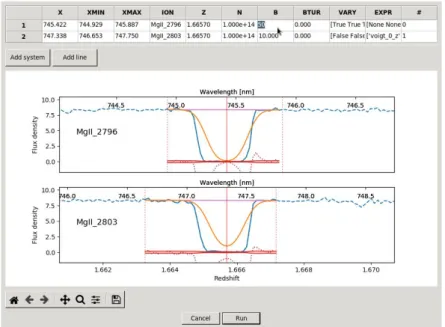
The dialog window of recipe Fit Selected System is more complex than the others, as shown in Fig.2. Here the top panel displays the group of lines belonging to a Mgii 2796-2803 system (as a database-style join from the entries of tables Lines and Systems), while the bottom panel displays the spectral regions to be considered when fitting the system itself (with wavelengths converted into redshifts). Through the dialog window the user can refine the model by editing the Voigt parameters in the table; any change is interactively reflected in the plot for immediate visual confirmation. Also the constraints on the parameter provided in the columns VARY and EXPR(which are automatically set to link the components of a system to each other; see Sec.3.3) can be edited at will. The best-fit parameters can be then computed by launching the recipe clicking on the Run button.

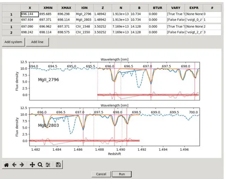
The Fit Selected System dialog window handles more complex cases, like composite (Fig.3) and blended systems (Fig. 4). In such cases, the table is split into two sub-panels, separating the selected system (top) from the others (bottom), which may be associated either to the same ionic transition (and thus be treated as members of a single complex systems together with the selected ones) or to a di↵erent one (and thus be treated as unrelated blended systems). Blended systems are automatically detected and considered together when modeling and fitting the line profiles; in this case, there is no di↵erence in running the procedure on any one of the blended system (e.e. the system in Fig.4would have been fitted in the exact same way selecting one of the two Mgii systems instead of the Civ one as a starting point). Clicking on the Add System and Add Line buttons the user can add terms to the composite profile, tweak the parameters to improve the model, and run the recipe to compute the best-fitting values.

(10)

X XMIN XMAX ION 2 N B BTUR

1 745.422 794.929 745.887 F19112796 1.66570 1.0090+14EE 0.000 True True 1/None None

2 747.338 746.653 747.750 F19112803 1.66570 1.000e+14 10.00 0.000 False Falsorvoigt 0 z'

N

Add system Add I ne

Wavelength him] 10.0 7.5 74-5 95.5 796.0 746.5 5.0 Mg11_2796 2.5 0.0 Wavelength him] 796.9 797.0 797.5 798.0 798.,g 7.5 5.0 _{Mg11_2803} 2.5 0.0 1.662 1.669 1.666 1.668 1.670 Redshift Run I

XMIM XMAX ION N B BTUR VARY EXPR 738.723 738.344 739.645 CIV_1548 3.77125 4.325e +13 5.920 0.000 [Tue Tme l [None None 0 2 739.953 739.645 740.786 CIV_1550 3.77125 4.325e +13 5.920 0.000 [False Falot l'voigt_ó Y 1 3 738.859 738.344 739.695 CIV_1548 3.77212 2.0340 +14 3.811 0.000 [Tue Tue l [None None 2

4 740.089 739.645 740.786 CIV_1550 3.77212 2.0340 +14 3.811 0.000 [False Falot ['voigt 2 z' 3 5 738.859 738.344 739.645 CIV_1548 3.77245 2.3090 +14 5.394 0.000 [Tue Tue l [None None 4

6 740.107 739.645 740.786 CIV_1550 3.77245 2.3090 +14 5.394 0.000 [False Falot ['voigt_4_z' 5 T 739.049 738.344 739.645 CIV_1548 3.77372 9.8170 +13 96.196 0.000 [Tue Tue l [None None 6

B 740.279 739.645 740.786 CIV_1550 3.77372 9.8170 +13 96.196 0.000 IFalse Falot ['voigt 6 z' 7 Add system Add line

10.0 z. 7.5 5.0 2.5 0.0 10.0 7.5 5.0 2.5 0.0 Wavelength Inm[ 738.2 L138.4

-"

738.6 7388 739.0 739.2 739.9 739.6 CIV_1544 Wavelength [nm] 739.4 739.6: 739.8 740.0 740.2 740.4 740.6 740.8 DV1550 3.768 3.770 Can 3.7 2 Retlshift Run I 3.774 3.776

Figure 2. The Fit Selected System dialog window, displaying a Mgii 2796-2803 system modeled with a Voigt profile:

the model is a very rough guess; the best-fit parameters can be computed by clicking on Run. The blue line is the observed flux density (dashed outside the fitting region), the purple line shows the position of the guess continuum, while the orange line shows the current model for the line profiles. Residuals (dotted red line) are compared with the error band on the flux density (solid red lines). [For colors, please refer to the digital copy].

Figure 3. The Fit Selected System dialog window, displaying a Civ 1548-1550 system fitted with a 4-component

(11)

X XMIN XMAX ION 2

1 696.144 695.685 696.298 Mg11_2796 1.48942 1.913e+13la 734 a000 rrue True 1/None None 0

a 697.934 697.371 698.114 N19112803 1.48942 1.913e+1310.734 aim /False Falservoigt 0 s.1

1 697.090 696.962 697.371 CIV_1548 3.50252 7.169e+1314.128 0.000 rrue Traci/None None2 2 698.292 698.114 698.575 CIV 1550 3.50252 7.169e+13 14.128 0.000 /False Falservoigt 2 z.3

Add system Add line

7.5 5.0 12.5 10.0 Wavelength Inm] 2.5 0.0 12.5 10.0 5.0 2.5 00 ?pi.a....,,,t.L...,.. Mg11_2796 ,....7.5.5 1 696.0 : 696.5 697. 697.5 698.0 I V 1

r

i ; , Wavelength Inml 696.0 696.5 697. 697.5 sga.d 698.5 699.0 699.5 700.0

,./

Mg 803 11-tes li 1 1 ; 1.482 1.484 tv (a E I ml 1.486 1.488 1.490 Redshat Run 1.492 1.494 1.496

Figure 4. The Fit Selected System dialog window, displaying a blended Civ 1548-1550 – Mgii 2796-2803 system,

with its best-fit Voigt profile. Same legend as Fig.2.

Adding systems or blended lines to improve the composite model chi-squared-wise is a procedure can be automatized via scripting, using the methods of the System class. The pattern of residuals can be used in this case to guess the parameters of the systems to be added. Such procedure is currently being implemented as a recipe accessible through the Astrocook GUI.

5. FUTURE PERSPECTIVE

The porting of the functionalities of the ESPRESSO DAS to Astrocook is still ongoing. A list of the soon-to-be implemented features includes:

• additional methods to guess and refine the estimation of the continuum (power-law fitting, modeling of the optical depth in the Lyman forest,8_etc.);

• ranking of the candidate absorption systems by likelihood (with an algorithm similar to the one described in22);

• identification of systems at the limit of detectability (by comparing a theoretical model with the observed flux density and looking for minima in the chi-squared values obtained along the spectrum).

The last technique has proved to be e↵ective to increase the completeness of the system detection at low column densities. It entails the generation of mock spectra to assess the detection completeness, a feature which is also going to be integrated within the Astrocook package through a dedicated class.

The development will be generally aimed to increase the automation without losing control over the opera-tions, which require to be specifically tailored to individual science cases. Two main tools are being conceived:

• a validation widget, which will allow the user to freeze the recipe parameters after a successful manual run, and apply the execution to a catalogue of spectra in background;

(12)

Further ideas to enhance the Astrocook GUI are expected to come from the user community at large. Several additional GUI recipes are being considered for implementation; other will stem directly from the actual use experience, consolidating the goal of making Astrocook a tool to “cook a spectrum in a thousand ways”.

ACKNOWLEDGMENTS

G. C. would like to thank Serafina Di Gioia for her insightful feedback on the design of the Astrocook classes and her contribution to the proofreading of this article.

REFERENCES

[1] Pepe, F. et al., “ESPRESSO – An Echelle SPectrograph for Rocky Exoplanets Search and Stable Spectro-scopic Observations,” The Messenger 153, 6–16 (2013).

[2] Zerbi, F. M. et al., “HIRES: the high resolution spectrograph for the E-ELT,” in [Ground-based and Airborne Instrumentation for Astronomy V ], Proc. SPIE 9147, 914723 (2014).

[3] Cupani, G. et al., “E-elt hires the high resolution spectrograph for the e-elt: integrated data flow system,” in [Observatory Operations: Strategies, Processes, and Systems V ], Peck, A. B. and Seaman, R. L., eds., Proc. SPIE 9910, 991023 (2016).

[4] Martins, C. J. A. P., “The status of varying constants: a review of the physics, searches and implications,” Reports on Progress in Physics 80(12), 126902 (2017).

[5] Sandage, A., “The Change of Redshift and Apparent Luminosity of Galaxies due to the Deceleration of Selected Expanding Universes.,” ApJ 136, 319 (1962).

[6] Di Marcantonio, P. et al., “Challenges and peculiarities of ESPRESSO data flow cycle: from target choice to scientific results,” in [Observatory Operations: Strategies, Processes, and Systems IV ], Peck, A. B., Seaman, R. L., and Comeron, F., eds., Proc. SPIE 8448, 84481O (2012).

[7] Cupani, G. et al., “Data Analysis Software for the ESPRESSO Science Machine,” in [ADASS XXIV], Taylor, A. R. and Rosolowsky, E., eds., ASP Conf. Ser. 495, 289 (2015).

[8] Cupani, G. et al., “Integrated data analysis in the age of precision spectroscopy: the espresso case,” in [Software and Cyberinfrastructure for Astronomy III ], Chiozzi, G. and Guzman, J. C., eds., Proc. SPIE 9913, 99131T (2016).

[9] Cupani, G. et al., “Field tests for the espresso data analysis software,” in [ADASS XXV], in press (2016). [10] Cupani, G. et al., “From espresso to the future – analysis of qso spectra with the astrocook package,” in

[ADASS XXVI ], in press (2017).

[11] Rossum, G., “Python reference manual,” tech. rep., Amsterdam, The Netherlands, The Netherlands (1995). [12] Jones, E., Oliphant, T., Peterson, P., et al., “SciPy: Open source scientific tools for Python,” (2001–2018).

Online; accessed 11 May 2018.

[13] Newville, M., Stensitzki, T., Allen, D. B., and Ingargiola, A., “LMFIT: Non-Linear Least-Square Minimiza-tion and Curve-Fitting for Python,” (2014).

[14] Astropy Collaboration, “Astropy: A community Python package for astronomy,” A&A 558, A33 (2013). [15] Freudling, W. et al., “Automated data reduction workflows for astronomy. The ESO Reflex environment,”

A&A 559, A96 (2013).

[16] McKay, D. J. et al., “The common pipeline library: standardizing pipeline processing,” in [Optimizing Scientific Return for Astronomy through Information Technologies ], Quinn, P. J. and Bridger, A., eds., Proc. SPIE 5493, 444–452 (2004).

[17] “Specutils.” https://github.com/astropy/specutils. Online; accessed 11 May 2018.

[18] Fontana, A. and Ballester, P., “FITLYMAN: a Midas tool for the analysis of absorption spectra.,” The Messenger 80, 37–41 (1995).

[19] Carswell, R. F. and Webb, J. K., “Voigt profile fitting program,” (1992–2016). Online; accessed 11 May 2018.

[20] Krogager, J.-K., “VoigtFit: A Python package for Voigt profile fitting,” ArXiv e-prints (2018).

[21] Hunter, J. D., “Matplotlib: A 2d graphics environment,” Computing In Science & Engineering 9(3), 90–95 (2007).

(13)

[22] Aaronson, M., McKee, C. F., and Weisheit, J. C., “The identification of absorption redshift systems in quasar spectra,” ApJ 198, 13–30 (1975).